Indicator Variograms as an Aid for Geological Interpretation and Modeling of Ore Deposits

1
Department of Mining Engineering, University of Chile, Santiago 8370448, Chile
2
Advanced Mining Technology Center, University of Chile, Santiago 8370448, Chile
*
Author to whom correspondence should be addressed.
Minerals 2017, 7(12), 241; https://doi.org/10.3390/min7120241
Submission received: 1 November 2017
/
Revised: 28 November 2017
/
Accepted: 30 November 2017
/
Published: 5 December 2017
(This article belongs to the Special Issue Geological Modelling)
Abstract
:Geostatistics offers a set of methods for modeling, predicting, or simulating geological domains in space. In addition of being an input of some of these methods, indicator direct and cross-variograms convey valuable information on the geometry of the domain layouts and on their contact relationships, in particular, on the surface area of a domain boundary, on the surface area of the contact between two domains, on the propensity for a domain to be in contact with, or separated from, another domain, and on the minimum and maximum distances between points from two domains. Accordingly, the indicator variograms inferred from sparse sampling data can be used to determine whether or not an interpreted model of the subsurface is consistent with the sampling information. The previous concepts are illustrated through a case study corresponding to a porphyry copper deposit.
1. Introduction
Identifying and modeling rock type, mineralization and alteration domains in ore deposits has become a crucial step in the assessment of geological and geometallurgical regionalized variables, such as metal grades or metal recoveries, due to the controls that these domains often exert on the distribution of these variables [1,2,3,4,5].
One issue for mining geologists and geometallurgists is to define the layout of each domain with the greatest possible accuracy, in order to minimize misclassifications (material predicted as belonging to a domain, but actually belonging to another one). Another issue relates to the consistency between the interpreted domain layouts and the information obtained from sampling data, so as to determine whether or not the geological interpretation is a faithful representation of reality. Of particular interest are the spatial regularity of the domain layouts and the contact relationships between domains, as some domains may have a propensity to be or not to be in contact depending on the geological setting.
The appraisal of the spatial and geometrical properties of geological domains often relies on geostatistical tools like vertical or regionalized proportion curves [6,7], contact matrices [8], transition probabilities under Markov chain models [9,10], or multiple-point metrics [11,12]. This paper focuses on alternative tools (namely, the indicator direct and cross-variograms) that are often disregarded in the geological modeling stage, although they can easily be inferred from a set of sampling data. The aim is to show that these tools convey geometrical information about the domain layouts and can be used to validate the consistency between sampling data (geological logs) and an interpreted geological model.
The outline is the following one: Section 2 provides theoretical background about the direct and cross-variograms of the indicators of non-overlapping domains and links the variogram properties with geometrical features of the domains. Section 3 presents a case study of a porphyry copper deposit. A general discussion and conclusions follow in Section 4 and Section 5, respectively.
2. Materials and Methods
2.1. Indicator Modeling
A geological model can be viewed as a partition of a mineral deposit or, more generally, of a region in the subsurface, into non-overlapping domains, such as rock type, mineralization or alteration domains. Each domain Dk, with k = 1, …, K, can be codified by a binary variable called indicator:
where x stands for a generic point in the three-dimensional Euclidean space R3. Viewing this indicator as a spatial random field in R3 opens the way for the use of the geostatistical formalism, which allows for prediction or simulation of the indicator at any point based on the values observed at surrounding sampling points.
The expected value of Ik(x) represents the probability of finding domain Dk at point x:
where E and P denote the expected value and the probability measure associated with the random field definition, respectively. Provided that the indicator random field is first-order stationary, pk does not depend on x and stands for the proportion of space covered by domain Dk. First-order stationarity means that the probability of finding domain Dk is constant over space.
2.2. Theoretical Indicator Direct Variogram
A tool commonly used in geostatistical modeling for quantifying the spatial continuity of domain Dk is the direct variogram of the indicator random field Ik, defined for each pair of points (x,x′) as:
where var denotes the variance. Under the assumption of first-order stationarity, one has [13,14,15]:
Furthermore, , so that one obtains:
Provided that the indicator random field Ik is second-order stationary, only depends on the separation vector between x and x′ and is commonly denoted as with h = x − x′. The indicator direct variogram represents the probability of transitioning from inside Dk at point x to outside Dk at point x′ = x − h (equivalently, from outside Dk at point x to inside Dk at point x − h), the transition happening somewhere over the extent of the separation vector h.
When the norm of x − x′ becomes infinitely large, the indicator variables Ik(x) and Ik(x′) are independent, so that . For separation vectors with a large norm, the indicator direct variogram presents a sill, whose value relates to the proportion of space (pk) covered by domain Dk:
The distance at which the indicator direct variogram reaches the sill (correlation range), corresponds to the distance beyond which the two indicator variables Ik(x) and Ik(x + h) are independent. This distance may depend on the direction of h and does not relate to the size of domain Dk [9] (under the first-order stationarity assumption, Dk has a constant probability of occurrence over R3, so it is unbounded) nor to the size of its convex parts [16] (based on Equation (5), Dk has the same indicator direct variogram as its complement, whose convex parts differ from that of Dk).
More information on the geometry of domain Dk can be obtained from the indicator direct variogram, in particular, from its behavior at the origin. The first-order derivative conveys information about the regularity of the boundary of Dk [13,17]:
where is the expected surface area of the boundary of Dk per unit volume of R3, S3 is the unit sphere of R3, u a unit-length vector and is the first-order derivative of the variogram at the origin in the direction of vector u:
Accordingly, unless Dk is void (pk = 0) or fills the whole space R3 (pk = 1), a null derivative (indicator direct variogram with a zero slope at the origin) in every direction cannot be observed [18]. A finite non-zero derivative means that the boundary of Dk is almost always regular (Figure 1A,B), while an infinite derivative means that Dk has an irregular or fractal boundary (Figure 1C,D). In the former case, the second-order derivative of the indicator direct variogram at the origin in the direction of vector u relates to the existence of singular points along the boundary of Dk [19]:
If the boundary has singular points (such as angular points or “vertices”), then the second-order derivative is negative and the indicator direct variogram is strictly concave near the origin (Figure 2A,B). On the contrary, if any point of the boundary has a single tangent plane (i.e., if Dk has a smooth boundary everywhere), then the second-order derivative of the indicator direct variogram at the origin is zero, which means that the variogram is straight at the origin (Figure 2C,D).
Finally note that the properties of the indicator direct variogram (correlation range, slope at the origin, concavity at the origin and overall shape) can depend on the direction of space under consideration, which corresponds to an anisotropic behavior of the indicator random field Ik. In such a case, the geometric properties of domain Dk and of its boundary are not the same in all the directions of space.
2.3. Experimental Indicator Direct Variogram
Given a set of points {} where the indicator is known, the experimental indicator direct variogram is defined as:
where N+(h) = { up to distance and angle tolerances} and card{N+(h)} is the cardinality of N+(h). Under a second-order stationarity assumption, this is an unbiased estimator of the indicator direct variogram , so that its properties (behavior at large distances, behavior near the origin, anisotropy) should be the same, up to statistical fluctuations.
An experimental variogram that does not converge to a positive sill may incite one to revise the second-order stationarity assumption. This situation happens when the probability of occurrence of Dk is not constant in space (presence of a systematic trend or zonation, which can be explained by geological considerations). In such a situation, one may assume that the second-order stationarity assumption is valid only at small scales (local stationarity), and restrict the interpretation of the experimental variogram to small distances. In particular, the regularity and smoothness of the domain boundary can still be inferred from the behavior of the variogram near the origin.
2.4. Theoretical Indicator Cross-Variogram
Consider now two domains Dk and Dk′ that do not overlap. The joint behavior of these two domains can be modeled by the cross-variogram of the associated indicator fields Ik and Ik′:
where cov denotes the covariance. Under the assumption of first-order stationarity, one has [14,15,16]:
The indicator cross-variogram is negative and represents, up to the sign, the probability of transitioning from Dk to Dk′ (or vice-versa, from Dk′ to Dk) between two points separated by vector h. If the two indicator random fields Ik and Ik′ are jointly second-order stationary, only depends on h = x – x′ and is commonly denoted as .
When the norm of x − x′ becomes infinitely large, the indicator variables Ik(x) and Ik′(x) are independent of Ik(x′) and Ik′(x′), so that [14]:
The indicator cross-variogram presents a sill whose value relates to the proportions of space covered by domains Dk and Dk′. The distance at which the sill is reached (correlation range) corresponds to the distance beyond which the indicator variables Ik(x) and Ik′(x) are independent of Ik(x + h) and Ik′(x + h). This distance may differ from the correlation ranges of the indicator direct variograms and may also depend on the direction of h. Note that the two domains Dk and Dk′ cannot be independent, insofar as they are assumed not to overlap; as a consequence, the cross-variogram cannot be identically zero, which is corroborated by the existence of a negative sill (Equation (13)), unless one of the domains is void (pk = 0 or pk′ = 0).
The behavior at the origin of the indicator cross-variogram conveys information about the boundary common to both domains Dk and Dk′. In particular, one has:
where is the expected surface area of the boundary common to Dk and Dk′ per unit volume of R3 and is the first-order derivative of the indicator cross-variogram at the origin in the direction of vector u:
A null derivative (indicator cross-variogram with a zero slope at the origin) in all directions indicates that Dk and Dk′ have no contact (Figure 3A,B). Even more, the distance up to which the cross-variogram is equal to zero in a given direction represents the minimum separation distance between the two domains Dk and Dk′ along this direction. In contrast, an indicator cross-variogram with a negative derivative (negative slope) at the origin indicates the existence of contacts between Dk and Dk′: the greater the slope, the more contact area exists (Figure 3C–F).
2.5. Experimental Indicator Cross-Variogram
Given a set of points {} where the indicators are known, the experimental indicator cross-variogram is defined as:
with the same notation as in Section 2.3. Under a second-order stationarity assumption, this is an unbiased estimator of the indicator cross-variogram and should therefore exhibit the same properties, up to statistical fluctuations.
An experimental indicator cross-variogram that does not converge to a negative sill may incite one to revise the second-order stationarity assumption. For instance, if Dk and Dk′ are bounded, the experimental indicator cross-variogram will be zero for distances larger than the maximum separation distance between points from the two domains (all the terms in the summation of Equation (16) are equal to zero). As stated in Section 2.3, one may then assume that the second-order stationarity assumption is valid only locally and restrict the interpretation of the experimental indicator cross-variogram to small distances. In particular, the slope at the origin reflects the amount of contact area between Dk and Dk′.
2.6. Link between Indicator Direct and Cross-Variograms
Due to the compositional nature of the indicator random fields, the sum of the indicator cross-variograms for is equal to the opposite of the indicator direct variogram , which can be demonstrated using Equations (5) and (12):
2.7. Ratio of Indicator Cross-to-Direct Variograms and Edge Effects
Under the assumption of first-order stationarity, based on Equations (5) and (12), the cross-to-direct variogram ratio corresponds, up to the sign, to the average probability of reaching domain Dk′ at point x′ when leaving Dk at point x or, vice-versa, of reaching domain Dk′ at point x when leaving Dk at point x′:
If the indicator random fields are second-order stationary, this ratio can be rewritten as:
with = 1 or −1 with equal probability 0.5. The sill of this ratio is (Equations (6) and (13)) [15]:
and corresponds, up to the sign, to the probability that a point x’ belongs to Dk′ knowing that it does not belong to Dk, which is equal to the proportion of domain Dk′ relative to the proportion of what is not Dk. Such a sill value can be used as a reference to determine whether or not the transition from domain Dk to domain Dk′ between two points separated by vector h or −h is preferential, a situation known as an edge effect or a border effect [14,20]. In particular, for small separation vectors ( with u a unit vector and a scalar tending to zero), the following cases may be found (Figure 4):
- : due to Equations (19) and (20), where is a point located close to x. Knowing that x belongs to Dk decreases the probability that x’ belongs to Dk′, given that it does not belong to Dk This means that the contact area between Dk and Dk′ is smaller than it would be in the absence of edge effect, i.e., there is a propensity for both domains not to be in contact (Figure 4A,B).
- : the contact area between domains Dk and Dk′ coincides with the expected contact area in the absence of edge effect (no preferential contact) (Figure 4C,D).
- : the contact area between Dk and Dk′ is larger than it would be in the absence of edge effect. There is a propensity for both domains to be in contact together (Figure 4E,F).
Because the indicator cross-to-direct variogram ratios for add to −1 (Equation (17)), the existence of an edge effect between domains Dk and Dk′ necessarily implies the existence of an opposite edge effect between Dk and Dk″ for some k″ {1, …, n}.
3. Case Study and Results
3.1. Presentation of the Deposit
The previous concepts are now illustrated through a case study corresponding to a porphyry copper deposit. For confidentiality reasons, the name and location of the deposit are not disclosed. The host rock is composed of a sequence of acidic and andesite volcanic rocks with intercalations of sedimentary rocks. Six main rock types have been recognized in the region under study (Figure 5):
- Andesite (code 1): this volcanic rock is distributed as an interbedded sequence spread over the whole deposit and consists of lavas, auto-breccias and ocoites, with porphyritic to aphanitic texture and, locally, with amygdaloidal to ocoitic texture.
- Other volcanic rocks (code 2): this is a sequence of differentiated volcanic rocks with textures that vary from porphyritic to tuffaceous with an aphanitic matrix.
- Sedimentary rocks (code 3): this rock type includes undifferentiated, volcaniclastic and calcareous sediments, which are mostly interbedded with dacite and andesite, forming the host rock of the intrusive porphyry.
- Granodioritic porphyry (code 4): this is a medium grain granodiorite of Triassic age.
- Monzonitic porphyry (code 5): this porphyry rock is associated with the hypogene mineralization.
- Hydrothermal breccia (code 6) with tourmaline, quartz, chalcopyrite and pyrite cements, which can be found in the contact between the monzonitic porphyry with the host rock as a breccia with intrusive fragments.
3.2. Data Presentation and Pre-Processing
The deposit has been recognized by a set of exploration diamond drill holes, along which the rock types have been logged. In the following, we will focus on a vertical cross-section in which 9060 data points are available, with information on the spatial coordinates and prevailing rock types of core samples. In addition to these data, a rock type model interpreted by the expert geologists is available (Figure 5).
In the forthcoming sections, the indicator direct and cross-variograms will be calculated, and geometrical information on the rock type layout will be extracted. To investigate the consistency of interpreted rock type model, the information obtained from the variograms calculated with the drill hole data will be compared with the information obtained from variograms calculated from the interpreted model.
To avoid misinterpretations, the experimental variograms calculated from the drill hole data are declustered to account for the irregular sampling pattern of these data [21,22,23]. To this end, each data is assigned a declustering weight equal to its area of influence within the corresponding rock type layout in the interpreted geological model. The weight assigned to a data pair in experimental variogram calculations corresponds to the product of the two data weights [21]. This way, the declustered mean (domain proportion) and variance (variogram sill) of each rock type indicator inferred from the drill hole data coincide with the mean and variance inferred from the interpreted model, facilitating the comparison between the indicator variograms calculated from the drill hole data and from the interpreted model.
3.3. Indicator Direct Variograms
For each rock type, the indicator direct variogram is calculated from the drill hole data and from the interpreted rock type model, along the directions experimentally recognized as the main directions of anisotropy (these are found to be the directions dipping 30° and −60° for rock types 1, 2 and 3, and the directions dipping −15° and 75° for rock types 4, 5 and 6, with the dip being measured positively upwards from the north direction). As an illustration, the direct variograms for rock types 1 (andesite) and 3 (sedimentary rocks) are displayed in Figure 6 and Figure 7, respectively. The following comments and interpretations can be made.
3.3.1. Existence of a Sill
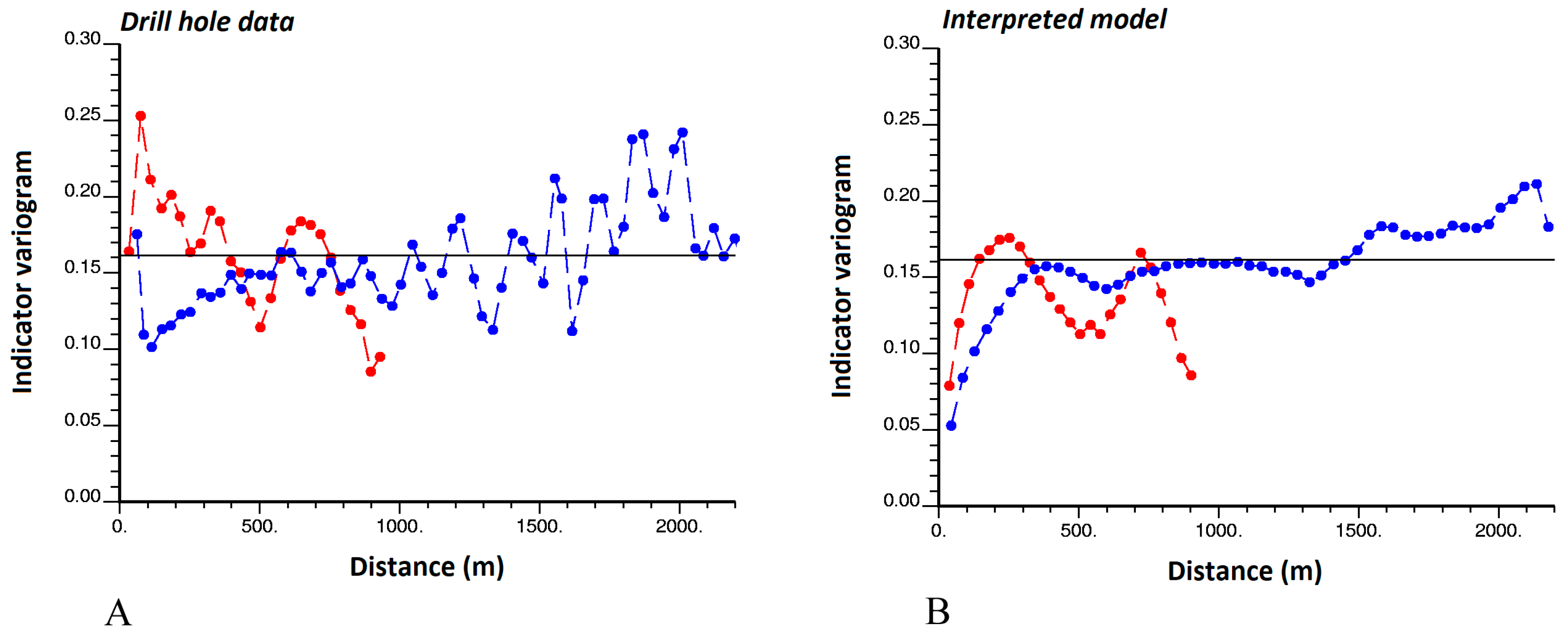
For both the drill hole data (Figure 6A) and the interpreted model (Figure 6B), the experimental indicator variogram of rock type 1 (andesite) does not converge to a sill, which makes the stationarity assumption questionable for this rock type. This is due to the fact that andesite mainly appears in the center of the region under study, so that its proportion is not constant in space. In contrast, the experimental indicator variogram of rock type 3 (sedimentary rocks) fluctuates around a sill (Figure 7), which agrees with the stationarity assumption at the working scale (2000–2500 m along the direction dipping 30° and 700–900 m along the direction dipping −60°). This assumption is reasonable, as the occurrences of sedimentary rocks are intermingled with that of the other rock types throughout the region under study. The variogram sill (0.16) is related to the proportion of the region covered by sedimentary rocks (0.20) (Equation (6)).
3.3.2. Shape and Anisotropy
Figure 6 and Figure 7 show that there is more spatial continuity along the direction dipping 30° than along the direction dipping −60°. The shapes of the experimental variograms calculated from the drill hole data (Figure 6A and Figure 7A) are comparable to those of the experimental variograms calculated from the interpreted geological model (Figure 6B and Figure 7B). In terms of spatial continuity, the interpreted model is therefore consistent with the drill hole data. As an exception, at short distances (0–300 m) along the direction dipping −60°, the experimental variograms calculated from the drill hole data increase faster than the experimental variograms calculated from the interpreted model, but this discrepancy can be provoked by statistical fluctuations and may not be significant.
3.3.3. Slope at the Origin
The experimental indicator variograms calculated from the drill hole data (Figure 6A and Figure 7A) have a large (almost infinite) slope at the origin; the same feature can be observed along other directions (not displayed in Figure 6 and Figure 7). This indicates that the boundaries of both andesite (rock type 1) and sedimentary rocks (rock type 3) are irregular (Equation (7)). The same indicator variograms calculated from the interpreted model (Figure 6B and Figure 7B) exhibit a more moderate slope at the origin and lower values at distances less than 100 m, suggesting slightly more regular domain boundaries and short-scale behavior. However, as mentioned above, the differences are deemed not significant in comparison with expected statistical fluctuations caused by the limited number of drill hole data, their irregular sampling design, and the possible presence of errors in the data (mislogged rock types in some drill hole samples). Several analytical and numerical approaches have been proposed to quantify experimental variogram fluctuations, based on resampling techniques or on the fitting of a theoretical random field model [24,25,26,27], which is out of the scope of this work.
3.4. Indicator Cross-Variograms
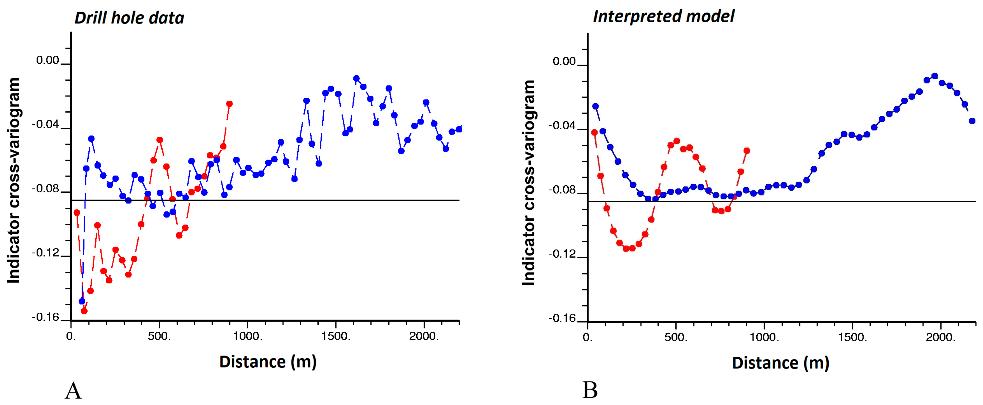
Let us now examine a few indicator cross-variograms calculated from the drill hole data (Figure 8A, Figure 9A and Figure 10A) and from the interpreted rock type model (Figure 8B, Figure 9B and Figure 10B) along the directions recognized as the main directions of anisotropy (directions dipping 30° and −60° for rock types 2 and 3; directions dipping −15° and 75° for rock types 4, 5 and 6).
3.4.1. Behavior at Large Distances
In case of joint second-order stationarity, the indicator cross-variogram should converge to a sill equal to minus the product of the rock type proportions (Equation (13)), but this behavior is not present in any of the three examples shown in Figure 8, Figure 9 and Figure 10. Instead, the presented cross-variograms tend to zero at large distances. As mentioned in Section 2.5, the distance at which an experimental indicator cross-variogram reaches a zero sill defines the maximum separation distance between points from the two associated rock types. It is deduced that points located in the other volcanic rocks (rock type 2) and sedimentary rocks (rock type 3) are distant no more than 1000 m along the direction dipping −60°, but can be distant more than 2000 m along the direction dipping 30° (Figure 8). Also, points located in granodioritic porphyry (rock type 4) are separated from points located in monzonitic porphyry (rock type 5) less than 800 m along the direction dipping 75° and 1200 m along the direction dipping −15° (Figure 9). Likewise, points located in granodioritic porphyry (rock type 4) are separated from points located in hydrothermal breccia (rock type 6) less than 1800 m along the direction dipping −15° (the two rock types are never found one above the other along the direction dipping 75°, as the corresponding cross-variogram is identically zero) (Figure 10).
3.4.2. Behavior at Short Distances
Since the associated indicator cross-variograms have a large negative slope at the origin, the other volcanic (rock type 2) and sedimentary (rock type 3) rocks on the one hand (Figure 8), and the granodioritic (rock type 4) and monzonitic (rock type 5) porphyries on the other hand (Figure 9) are in contact along the two anisotropy directions. In both cases, up to expected statistical fluctuations, the cross-variograms calculated from the interpreted model are comparable to the cross-variograms calculated from the drill hole data at short distances (0 to 300 m). Therefore, there is no evidence that the amounts of contacts between the rock type domains in the interpreted model are over- or underestimated with respect to reality: the interpreted model agrees with the sampling information in this aspect.
In contrast, it is observed that the indicator cross-variogram between granodioritic porphyry (rock type 4) and hydrothermal breccia (rock type 6) is zero until a distance of 1000 m (according to drill hole data, Figure 10A) or 500 m (according to the interpreted model, Figure 10B) along the direction dipping −15°. These figures indicate the minimum distance between both rock types along the mentioned direction, being twice larger in the drill hole data. A revision of the interpreted geological model is therefore advisable not to underestimate the true separation distance between granodioritic porphyry and hydrothermal breccia.
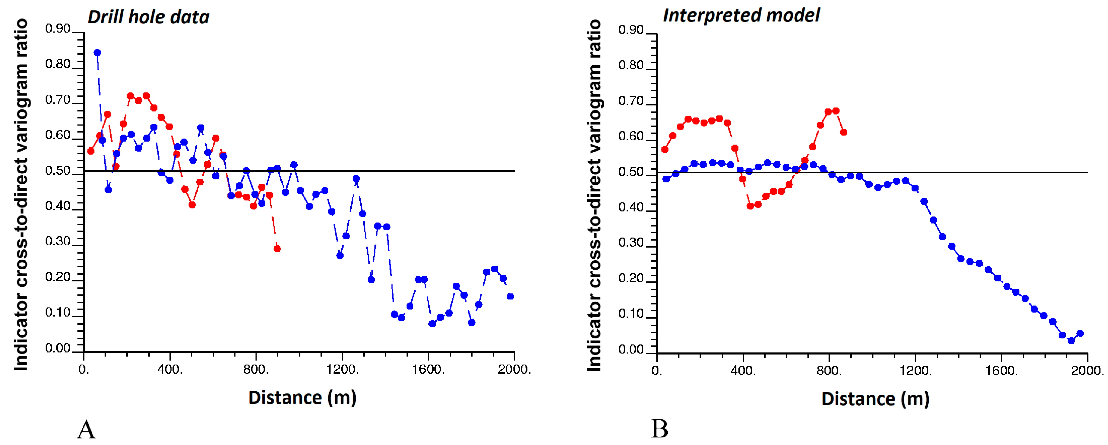
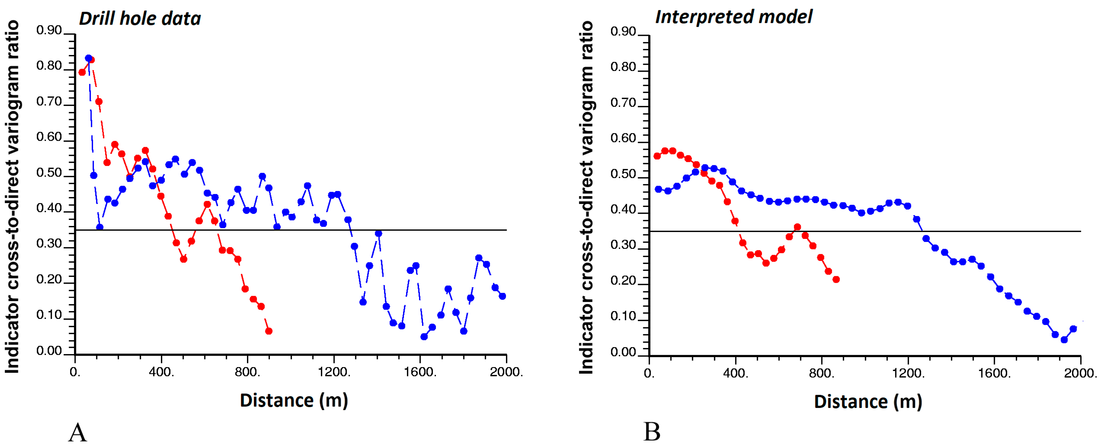
3.5. Ratios of Indicator Cross-to-Direct Variograms
We now focus on the ratios of indicator cross-to-direct variograms (Equation (19)). As an illustration, Figure 11 and Figure 12 show these ratios for rock types 2 (other volcanic rocks) and 3 (sedimentary rocks). From these two examples, one concludes that, at short distances, there is an edge effect between other volcanic and sedimentary rocks, with both domains being prone to be in contact, which can be corroborated by a look at the cross-section displayed in Figure 5. The edge effect is stronger when leaving the other volcanic rocks to reach the sedimentary rocks than in the opposite way, as the ratio plotted in Figure 11 is only a little higher than the expected sill, while the ratio in Figure 12 is significantly higher than the expected sill (one mostly finds rock type 3 when leaving rock type 2, while one mostly finds both rock types 1 and 2 when leaving rock type 3). Such edge effects can be explained by lithostratigraphic considerations, as the region is characterized by a volcano-sedimentary sequence consisting of volcanic rocks (mainly rhyolitic and dacitic ash-flow tuffs, pyroclastic rocks, as well as basaltic and andesitic lavas) followed by sedimentary intercalations, which imply spatial alternations between rock type 3 (sedimentary rocks) and rock types 1 and 2 (andesite and other volcanic rocks, respectively).
4. Discussion
4.1. Geological Interpretation and Modeling
A first axis for discussion concerns the geological domaining of ore deposits and the modeling of the domain layouts for further use in the evaluation of mineral resources and ore reserves or in the quantification of geological uncertainty. As shown in the previous sections, the indicator direct and cross-variograms give a profound insight into the spatial and geometrical properties of geological domains and into their contact relationships, since they convey information about the regularity and smoothness of the domain boundaries, the contact area between two domains, and their propensity to be in contact with, or separated from, each other at short distances.
Besides the aforementioned properties, one aspect not captured by indicator variograms is the presence of a directional edge effect, when the transition from a domain to another one preferentially occurs in one way rather than in the opposite way (for instance, an oxide mineralogical domain located above a sulfide domain, while the reverse does not happen). To investigate such an edge effect, it is necessary to resort to the indicator cross-covariance (Appendix A), which is not an even function, unlike the indicator cross-variogram.
Indicator variograms or covariances therefore appear as a helpful tool to determine whether or not an interpreted geological model is consistent with sampling data. For instance, a hand-drawn interpreted model that is intended to be a locally accurate representation of reality is likely to exhibit over-smoothed domain boundaries or to exaggerate the domain spatial continuity, a situation that should be avoided if the interpreted model is used as a reference (training image) for constructing multiple realizations of the geological domain layouts.
4.2. Geostatistical Modeling and Simulation
A second axis for discussion concerns the spatial prediction or simulation of geological domains for modeling the subsurface and quantifying geological uncertainty. Two types of geostatistical approaches have been developed for such a purpose. The first one consists of model-driven approaches, which rely on the definition of a categorical random field and the specification of the parameters characterizing its spatial distribution; the reader is referred to [13] for a review of the most widespread model-driven approaches. The second type is the family of data-driven approaches. These approaches do not completely specify the random field, but rely on the fitting of some of its parameters directly from the available data.
The latter approaches are likely to suffer from consistency problems in the definition of the model parameters. As a first example, indicator-based approaches such as indicator kriging, indicator cokriging or sequential indicator simulation [28] rely on the fitting of indicator variogram models. However, as seen in Section 2 and Section 3, the behaviors of the direct and cross-variograms near the origin is likely to be very different, with a possible zero slope for the cross-variograms, a situation that is prohibited for the direct variograms. The anisotropy directions and the behavior at large distances may also not be the same for the indicator direct and cross-variograms. In this context, the widely used linear model of coregionalization, based on the fitting of the direct and cross-variograms with the same set of basic nested structures [28,29], is inadequate. So is the separate modeling of the indicator direct variograms, as used in indicator kriging and in sequential indicator simulation, because it neglects the indicator cross-variograms and therefore omits important information about the contact relationships between the geological domains. Instead, a non-linear model of coregionalization should be used, a task that is made complex due to the mathematical restrictions that affect the indicator variograms [13,18,27]. As a second example, the simulation approaches based on multiple-point statistics [30] rely on the definition of a training image that is representative of the spatial distribution of the geological domains under study. Following the statements of the previous subsection, the choice of a training image consistent with the indicator direct and cross-variograms that can be inferred from available sampling data (in particular, reproducing the domain proportions, boundary regularity, contact relationships and edge effects) turns out to be crucial and non-trivial.
5. Conclusions
In geostatistical applications, geological domains are often codified through indicators and partially characterized by their direct and cross-variograms. The sills, correlation ranges, shapes and possible anisotropies of such indicator variograms convey information about the domain proportions and on their spatial correlation structure. Furthermore, their behavior at short distances brings a wealth of knowledge on the domain boundaries. In particular, the average slope at the origin is proportional to the surface area of the domain boundary (in case of a direct variogram) or to the surface area of the contact between two domains (in case of a cross-variogram): the more slope, the more surface area. Also, the ratio of cross-to-direct variograms allows identification for whether two domains are preferentially in contact (border or edge effect) or whether they tend to be separated. Finally, the range of distances for which an indicator cross-variogram differs from zero provides information about the minimum and maximum distances between points from two domains.
In practice, all of these properties can be investigated on the basis of sampling information, through the analysis of experimental indicator variograms. Such an analysis is helpful for validating the consistency of an interpreted geological model of the subsurface or for constructing a representative training image to be used for simulating the layout of the domains with data-driven geostatistical approaches based on multiple-point statistics. A case study of a copper ore deposit has been presented, in which the interpreted layout of rock type domains is globally consistent with the actual layout, as revealed from the analysis of exploration drill hole data; as an exception, the distance separating two rock type domains (granodioritic porphyry and hydrothermal breccia) may be underestimated in the interpreted model and needs to be revised.
Acknowledgments
The first two authors acknowledge the funding of the Chilean Commission for Scientific and Technological Research (CONICYT), through Projects CONICYT PIA Anillo ACT1407 and CONICYT/FONDECYT/REGULAR/N°1170101, respectively. Costs to publish in open access were covered by CONICYT/FONDECYT/REGULAR/N°1170101 funds.
Author Contributions
Mohammad Maleki, Xavier Emery and Nadia Mery conceived and designed the experiments; Mohammad Maleki performed the experiments; Xavier Emery wrote the paper.
Conflicts of Interest
The authors declare no conflict of interest. The founding sponsors had no role in the design of the study; in the collection, analyses, or interpretation of data; in the writing of the manuscript, and in the decision to publish the results.
Appendix A
Consider two domains Dk and Dk′ that do not overlap. The non-centered cross-covariance of the domains indicators Ik and Ik′ is defined as:
and is related to the indicator cross-variogram in the following fashion (Equation (12)):
If the two indicator random fields are jointly second-order stationary, Ck,k′ only depends on h = x′ − x and tends to pk pk′ when the norm of x′ − x becomes infinitely large. Furthermore, the boundary common to both domains Dk and Dk′ is related with the average derivative of Ck,k′ at the origin (Equation (14)):
Unlike the cross-variogram, the cross-covariance provides information on the directional contact between the two domains Dk and Dk′ and on asymmetrical relationships between these domains (for instance, Dk being preferentially above Dk′ rather than below), a pattern that can sometimes be explained by chemical or sedimentological processes [9,31,32]. In particular, the ratio between indicator cross-covariance and direct variogram is:
and corresponds, up to the sign, to the case of Equation (19). The sill of this ratio is pk′/(1 – pk) and represents the reference value against which one can determine the existence of directional edge effects at very small distances:
- : the contact area between Dk and Dk′ when moving along vector u (i.e., leaving Dk at x and reaching Dk′ at ) is smaller than it would be in the absence of a directional edge effect.
- : the contact area between Dk and Dk′ when moving along vector u is equal to the expected area in the absence of a directional edge effect.
- : the contact area between Dk and Dk′ when moving along vector u is larger than it would be in the absence of an edge effect.
References
- Dowd, P.A. Structural controls in the geostatistical simulation of mineral deposits. In Geostatistics Wollongong’96; Baafi, E.Y., Schofield, N.A., Eds.; Kluwer Academic: Dordrecht, The Netherlands, 1997; pp. 647–657. [Google Scholar]
- Vargas-Guzmán, J.A. Transitive geostatistics for stepwise modeling across boundaries between rock regions. Math. Geosci. 2008, 40, 861–873. [Google Scholar] [CrossRef]
- Rossi, M.E.; Deutsch, C.V. Mineral Resource Estimation; Springer: London, UK, 2014; p. 332. [Google Scholar]
- Madani, N.; Emery, X. Plurigaussian modeling of geological domains based on the truncation of non-stationary Gaussian random fields. Stoch. Environ. Res. Risk Assess. 2017, 31, 893–913. [Google Scholar] [CrossRef]
- Mery, N.; Emery, X.; Cáceres, A.; Ribeiro, D.; Cunha, E. Geostatistical modeling of the geological uncertainty in an iron ore deposit. Ore Geol. Rev. 2017, 88, 336–351. [Google Scholar] [CrossRef]
- Matheron, G.; Beucher, H.; de Fouquet, C.; Galli, A.; Guérillot, D.; Ravenne, C. Conditional simulation of the geometry of fluvio-deltaic reservoirs. In Proceedings of the SPE Annual Technical Conference and Exhibition, Dallas, TX, USA, 27–30 September 1987; Society of Petroleum Engineers: Richardson, TX, USA, 1987; pp. 591–599. [Google Scholar]
- Ravenne, C.; Galli, A.; Doligez, B.; Beucher, H.; Eschard, R. Quantification of facies relationships via proportion curves. In Geostatistics Rio 2000; Armstrong, M., Bettini, C., Champigny, N., Galli, A., Remacre, A., Eds.; Kluwer: Dordrecht, The Netherlands, 2002; pp. 19–40. [Google Scholar]
- Xu, C.; Dowd, P.A.; Mardia, K.V.; Fowell, R.J. A flexible true plurigaussian code for spatial facies simulations. Comput. Geosci. 2006, 32, 1629–1645. [Google Scholar] [CrossRef]
- Carle, S.F.; Fogg, G.E. Transition probability-based indicator geostatistics. Math. Geol. 1996, 28, 453–476. [Google Scholar] [CrossRef]
- Carle, S.F.; Fogg, G.E. Modeling spatial variability with one- and multidimensional continuous-lag Markov chains. Math. Geol. 1997, 29, 891–918. [Google Scholar] [CrossRef]
- Boisvert, J.B.; Pyrcz, M.J.; Deutsch, C.V. Multiple point metrics to assess categorical variable models. Nat. Resour. Res. 2010, 19, 165–175. [Google Scholar] [CrossRef]
- Dimitrakopoulos, R.; Mustapha, H.; Gloaguen, E. High-order statistics of spatial random fields: Exploring spatial cumulants for modeling complex non-Gaussian and non-linear phenomena. Math. Geosci. 2010, 42, 65–99. [Google Scholar] [CrossRef]
- Lantuéjoul, C. Geostatistical Simulation: Models and Algorithms; Springer: Berlin/Heidelberg, Germany, 2002; p. 256. [Google Scholar]
- Séguret, S.A. Analysis and estimation of multi-unit deposits: Application to a porphyry copper deposit. Math. Geosci. 2013, 45, 927–947. [Google Scholar] [CrossRef] [Green Version]
- Beucher, H.; Renard, D. Truncated Gaussian and derived methods. C. R. Geosci. 2016, 348, 510–519. [Google Scholar] [CrossRef]
- Armstrong, M.; Galli, A.; Beucher, H.; Le Loc’h, G.; Renard, D.; Doligez, B.; Eschard, R.; Geffroy, F. Plurigaussian Simulations in Geosciences; Springer: Berlin/Heidelberg, Germany, 2011; p. 176. [Google Scholar]
- Matheron, G. Eléments Pour une Théorie des Milieux Poreux; Masson: Paris, France, 1967; p. 166. [Google Scholar]
- Dubrule, O. Indicator variogram models: Do we have much choice? Math. Geosci. 2017, 49, 441–465. [Google Scholar] [CrossRef]
- Emery, X.; Lantuéjoul, C. Geometric covariograms, indicator variograms and boundaries of planar closed sets. Math. Geosci. 2011, 43, 905–927. [Google Scholar] [CrossRef]
- Roth, C. Incorporating information about edge effects when simulating lithofacies. Math. Geol. 2000, 32, 277–300. [Google Scholar] [CrossRef]
- Rivoirard, J. Weighted variograms. In Geostatistics 2000 Cape Town; Kleingeld, W.J., Krige, D.G., Eds.; Geostatistical Association of Southern Africa: Cape Town, South Africa, 2001; pp. 145–155. [Google Scholar]
- Emery, X.; Ortiz, J.M. Weighted sample variograms as a tool to better assess the spatial variability of soil properties. Geoderma 2007, 140, 81–89. [Google Scholar] [CrossRef]
- De Souza, L.E.; Costa, J.F.C.L. Sample weighted variograms on the sequential indicator simulation of coal deposits. Int. J. Coal Geol. 2013, 112, 154–163. [Google Scholar] [CrossRef]
- Emery, X. Reducing fluctuations in the sample variogram. Stoch. Environ. Res. Risk Assess. 2007, 21, 391–403. [Google Scholar] [CrossRef]
- Clark, R.G.; Allingham, S. Robust resampling confidence intervals for empirical variograms. Math. Geosci. 2011, 43, 243–259. [Google Scholar] [CrossRef]
- Olea, R.A.; Pardo-Igúzquiza, E. Generalized bootstrap method for assessment of uncertainty in semivariogram inference. Math. Geosci. 2011, 43, 203–228. [Google Scholar] [CrossRef]
- Chilès, J.P.; Delfiner, P. Geostatistics: Modeling Spatial Uncertainty; Wiley: New York, NY, USA, 2012; p. 699. [Google Scholar]
- Goovaerts, P. Geostatistics for Natural Resources Evaluation; Oxford University Press: New York, NY, USA, 1997; p. 480. [Google Scholar]
- Wackernagel, H. Multivariate Geostatistics: An Introduction with Applications; Springer: Berlin/Heidelberg, Germany, 2003; p. 388. [Google Scholar]
- Mariethoz, G.; Caers, J. Multiple-Point Geostatistics: Stochastic Modeling with Training Images; Wiley: New York, NY, USA, 2014; p. 376. [Google Scholar]
- Langlais, V.; Beucher, H.; Renard, D. In the shade of the truncated Gaussian simulation. In Proceedings of the Eighth International Geostatistics Congress, Santiago, Chile, 1–5 December 2008; Ortiz, J.M., Emery, X., Eds.; Gecamin Ltda: Santiago, Chile, 2008; pp. 799–808. [Google Scholar]
- Le Blévec, T.; Dubrule, O.; John, C.M.; Hampson, G.J. Modelling asymmetrical facies sucessions using pluri-Gaussian simulations. In Geostatistics Valencia 2016; Gómez-Hernández, J.J., Rodrigo-Ilarri, J., Rodrigo-Clavero, M.E., Cassiraga, E., Vargas-Guzmán, J.A., Eds.; Springer International Publishing AG: Cham, Switzerland, 2017; pp. 59–75. [Google Scholar]
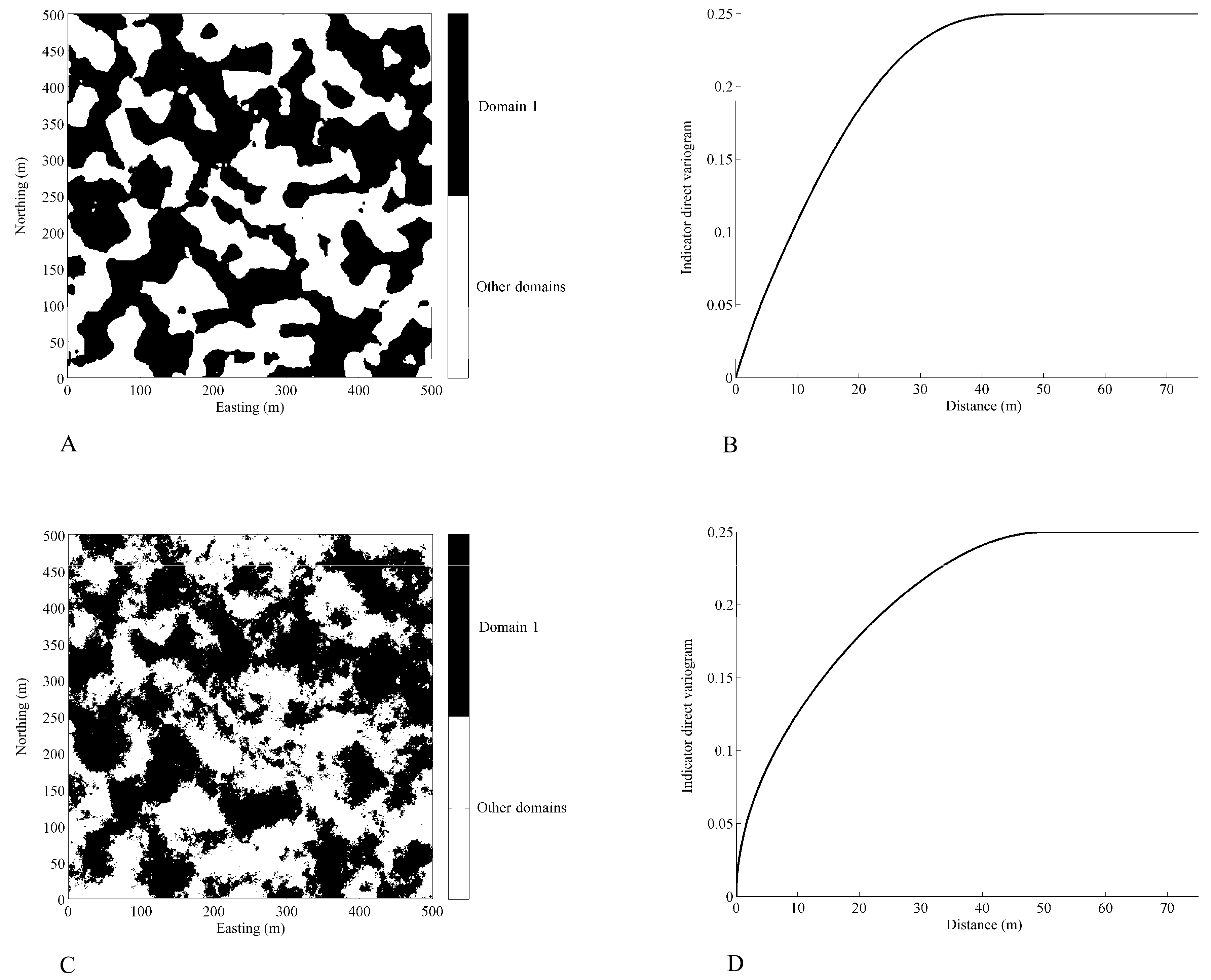
Figure 1.
Plan views of geological domains (A,C) and indicator variograms of domain D1 (B,D). The regularity of the domain boundary is reflected in the first-order derivative of the indicator direct variogram at the origin: regular domain boundary (A) associated with a finite variogram slope at the origin (B); fractal domain boundary (C) associated with an infinite variogram slope at the origin (D).

Figure 2.
Plan views of geological domains (A,C) and indicator variograms of domain D1 (B,D). The smoothness of the domain boundary is reflected in the second-order derivative of the indicator direct variogram at the origin: domain boundary with vertices highlighted in red (A) associated with a strictly concave variogram near the origin (B); smooth domain boundary (C) associated with a straight variogram near the origin (D).
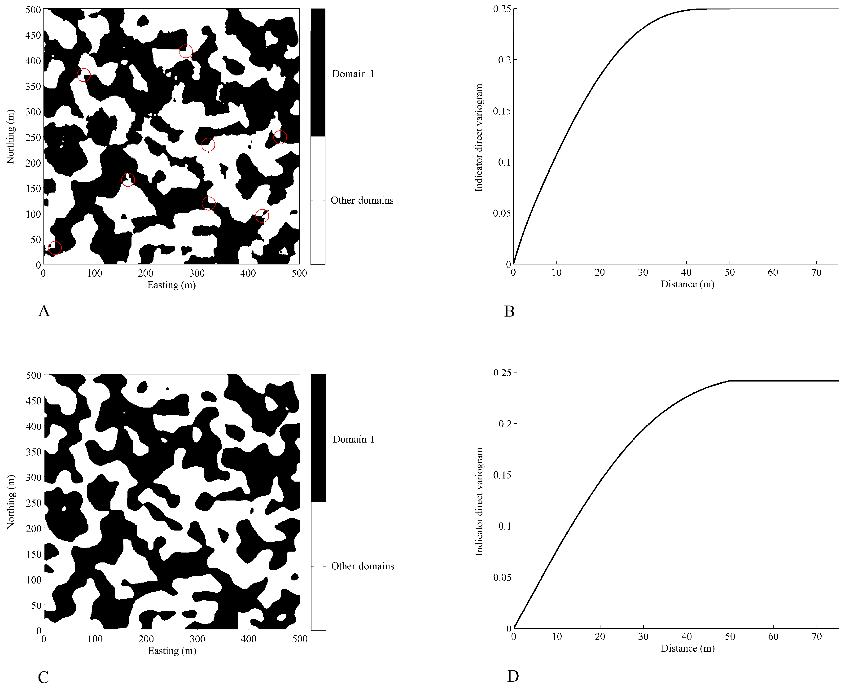
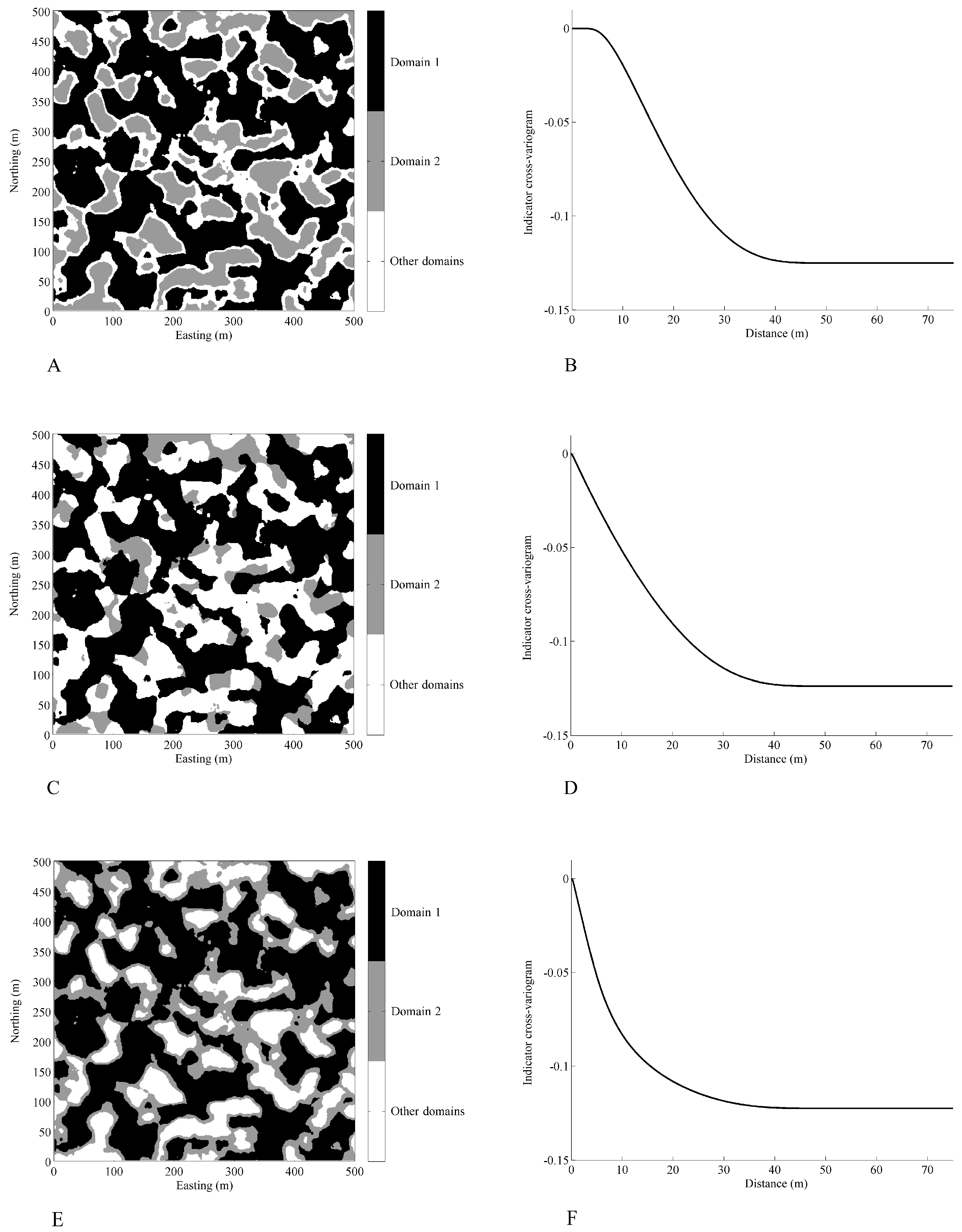
Figure 3.
Plan views of geological domains (A,C,E) and indicator cross-variograms of domains D1 and D2 (B,D,F). The surface area of the contact between domains D1 and D2 is reflected in the first-order derivative of the indicator cross-variogram at the origin: no contact between domains (A) associated with a zero cross-variogram slope at the origin (B); existence of a contact with a small surface area (C) associated with a small negative cross-variogram slope at the origin (D); existence of a contact with a large surface area (E) associated with a large negative cross-variogram slope at the origin (F).

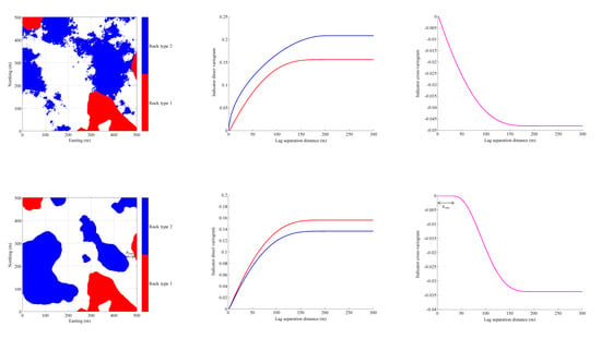
Figure 4.
Plan views of geological domains (A,C,E) and absolute values of the ratios of indicator cross-to-direct variograms (red curves) (B,D,F); the expected sill value (Equation (20)) is represented by a black solid line.
Figure 4.
Plan views of geological domains (A,C,E) and absolute values of the ratios of indicator cross-to-direct variograms (red curves) (B,D,F); the expected sill value (Equation (20)) is represented by a black solid line.
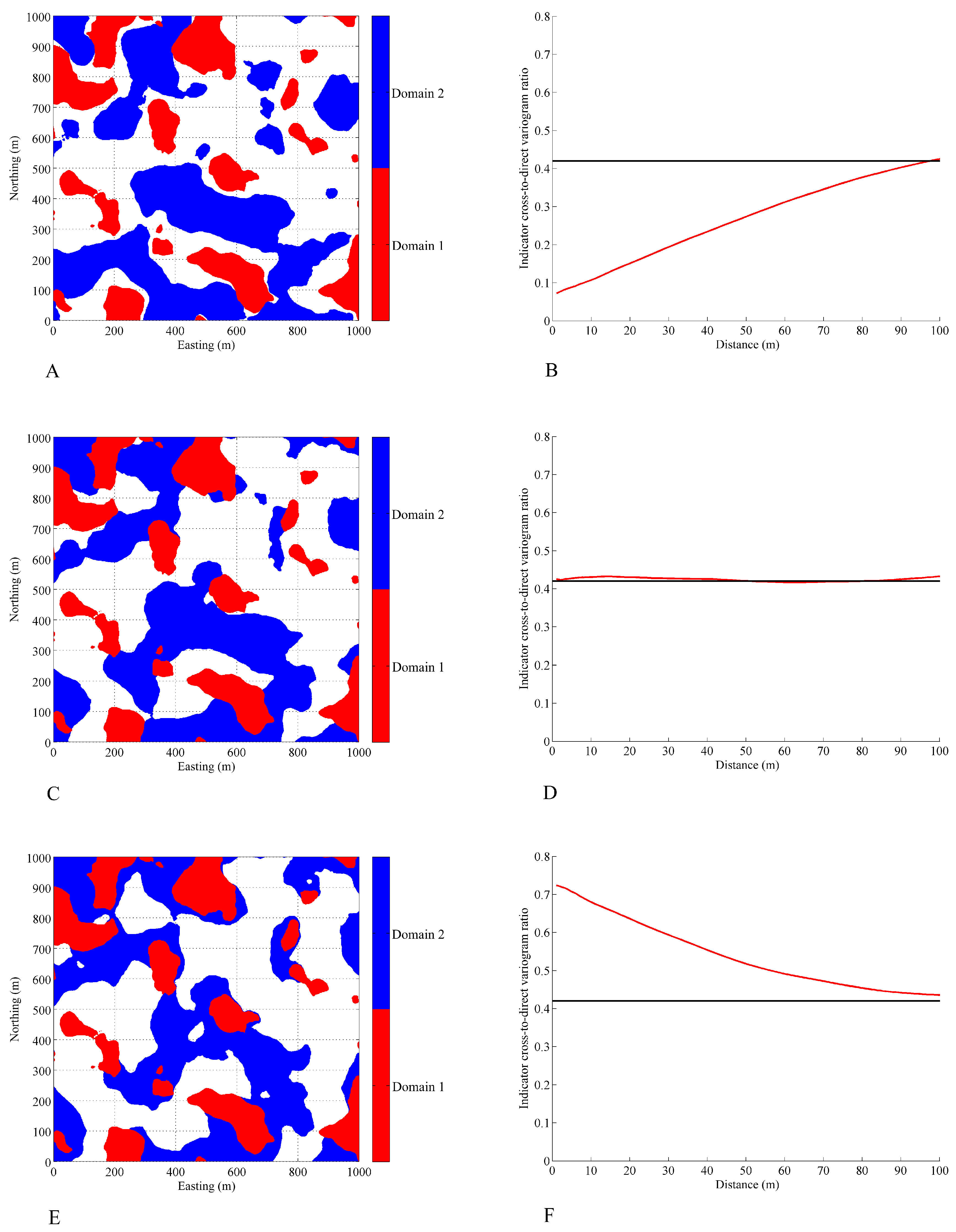
Figure 5.
Interpreted rock type model in a cross-section under study. Sample drill hole data have been superimposed. Local coordinates are used to preserve the confidentiality of the data.
Figure 5.
Interpreted rock type model in a cross-section under study. Sample drill hole data have been superimposed. Local coordinates are used to preserve the confidentiality of the data.
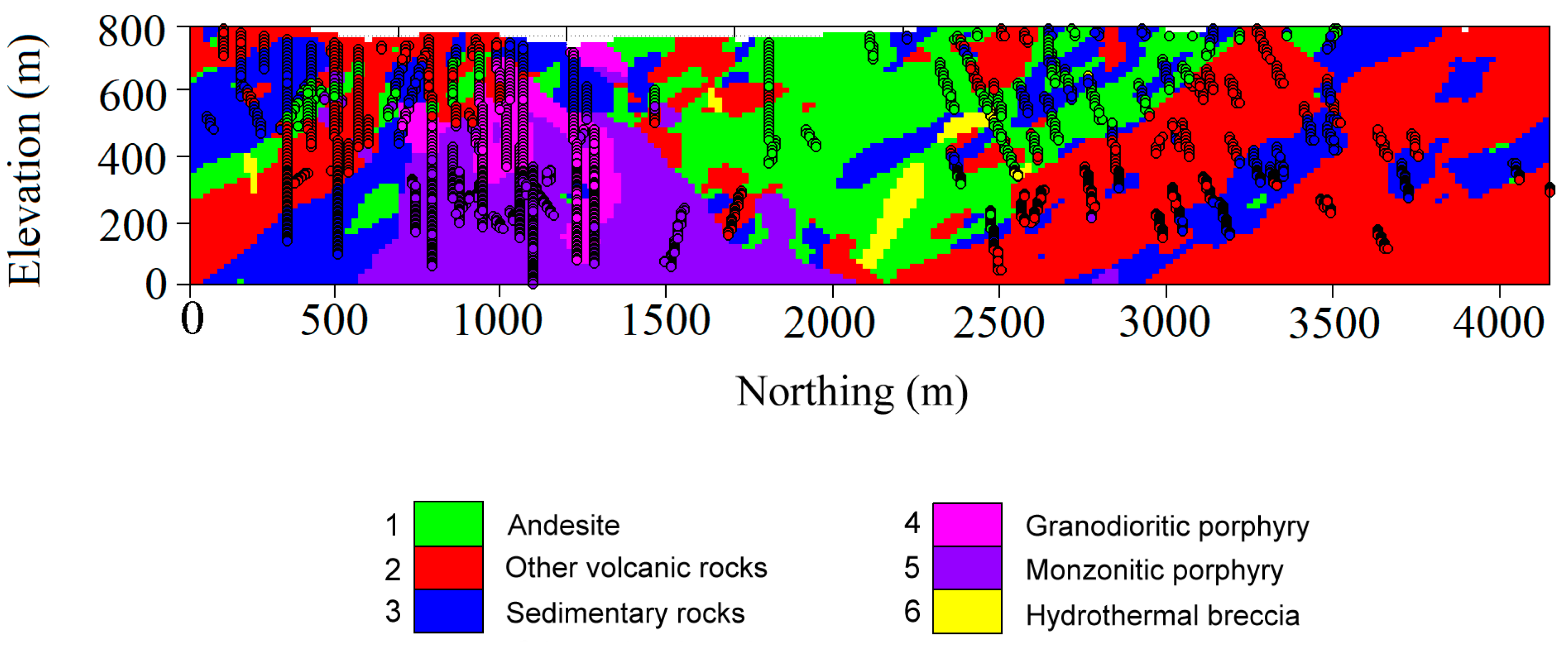
Figure 6.
Indicator direct variogram of rock type 1 (andesite) along directions dipping 30° (blue) and −60° (red) with respect to the north direction, calculated from (A) drill hole data, (B) interpreted model. Calculations consider an angle tolerance of 20° around the target directions. The same lag values have been used for both variograms.
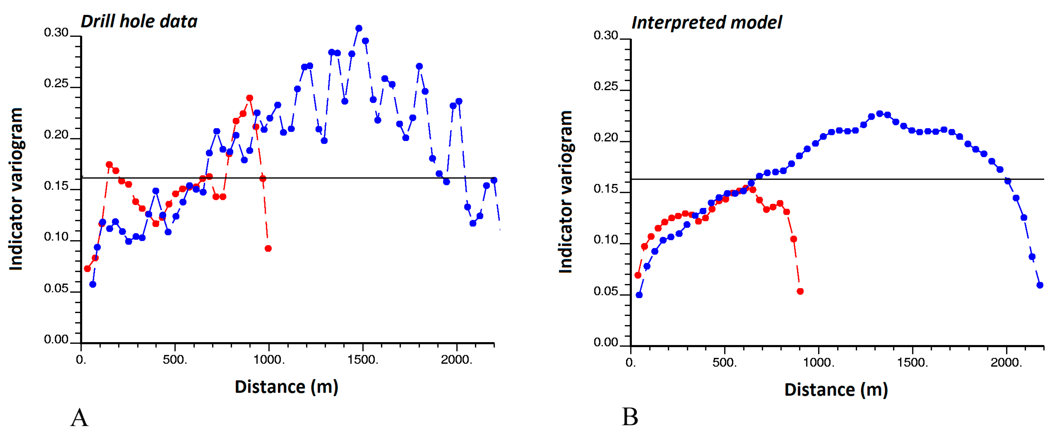
Figure 7.
Indicator direct variogram of rock type 3 (sedimentary rocks) along directions dipping 30° (blue) and −60° (red) with respect to the north direction, calculated from (A) drill hole data, (B) interpreted model. Calculations consider an angle tolerance of 20° around the target directions. The same lag values have been used for both variograms.

Figure 8.
Indicator cross-variogram between rock types 2 (other volcanic rocks) and 3 (sedimentary rocks) along directions dipping 30° (blue) and −60° (red) with respect to the north direction, calculated from (A) drill hole data, (B) interpreted model. Calculations consider an angle tolerance of 20° around the target directions. The same lag values have been used for both cross-variograms.

Figure 9.
Indicator cross-variogram between rock types 4 (granodioritic porphyry) and 5 (monzonitic porphyry) along directions dipping 75° (blue) and −15° (red) with respect to the north direction, calculated from (A) drill hole data, (B) interpreted model. Calculations consider an angle tolerance of 20° around the target directions. The same lag values have been used for both cross-variograms.
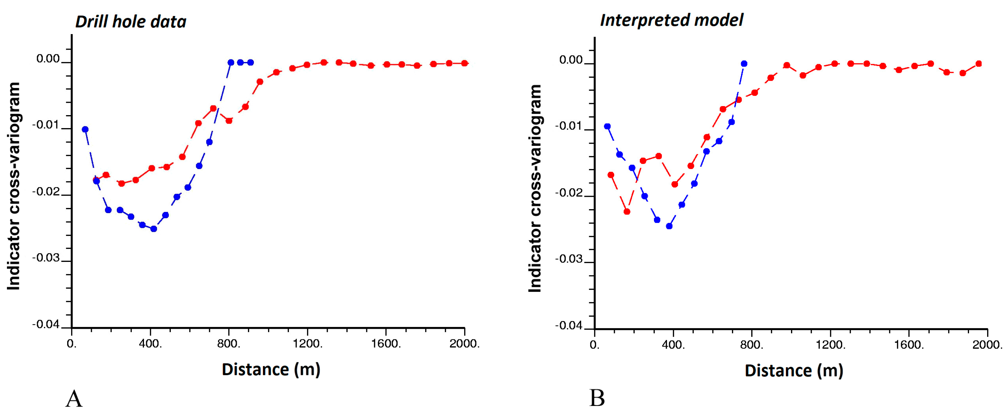
Figure 10.
Indicator cross-variogram between rock types 4 (granodioritic porphyry) and 6 (hydrothermal breccia) along directions dipping 75° (blue) and −15° (red) with respect to the north direction, calculated from (A) drill hole data, (B) interpreted model. Calculations consider an angle tolerance of 20° around the target directions. The same lag values have been used for both cross-variograms.
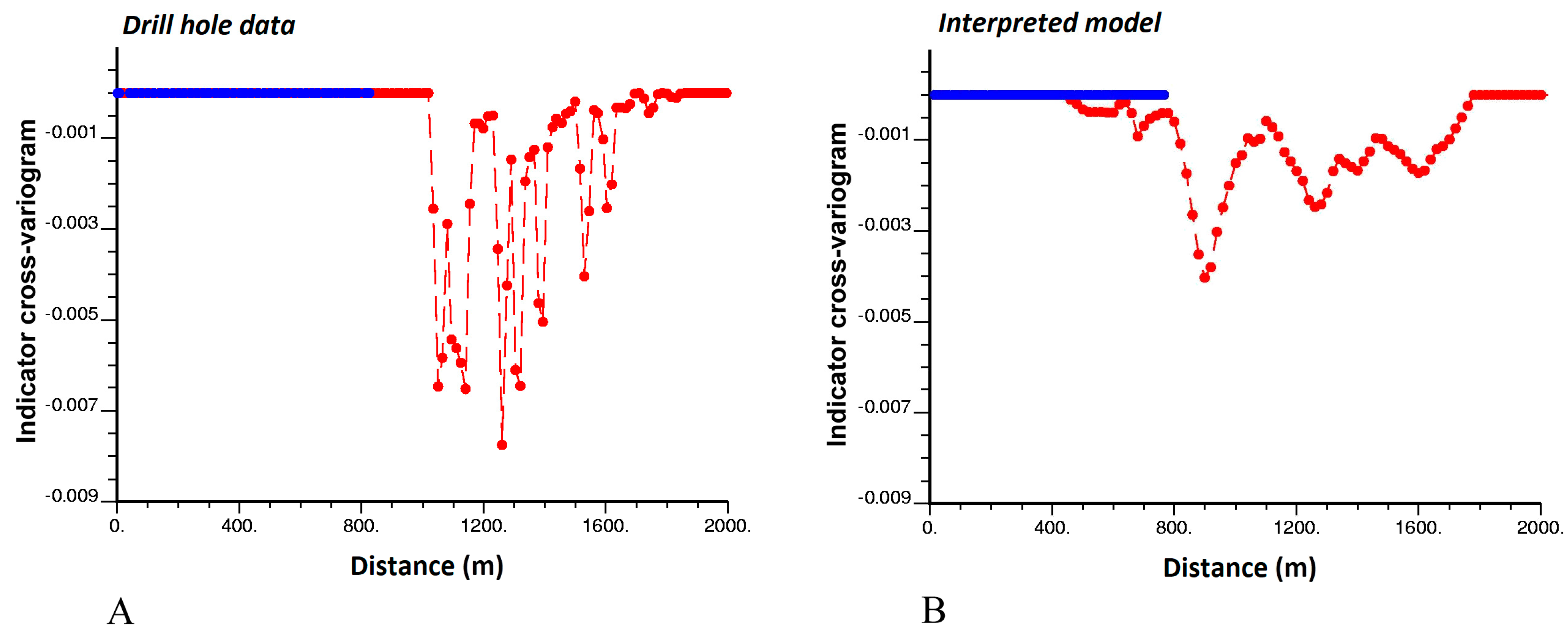
Figure 11.
Absolute value of the ratio of indicator cross-to-direct variograms between rock types 2 (other volcanic rocks) and 3 (sedimentary rocks) along directions dipping 30° (blue) and −60° (red) with respect to the north direction, calculated from (A) drill hole data, (B) interpreted model. Calculations consider an angle tolerance of 20° around the target directions. The same lag values have been used for both variogram ratios. The expected sill value (Equation (20)) is represented by a black solid line.

Figure 12.
Absolute value of the ratio of indicator cross-to-direct variograms between rock types 3 (sedimentary rocks) and 2 (other volcanic rocks) along directions dipping 30° (blue) and −60° (red) with respect to the north direction, calculated from (A) drill hole data, (B) interpreted model. Calculations consider an angle tolerance of 20° around the target directions. The same lag values have been used for both variogram ratios. The expected sill value (Equation (20)) is represented by a black solid line.

© 2017 by the authors. Licensee MDPI, Basel, Switzerland. This article is an open access article distributed under the terms and conditions of the Creative Commons Attribution (CC BY) license (http://creativecommons.org/licenses/by/4.0/).
Share and Cite
MDPI and ACS Style
Maleki, M.; Emery, X.; Mery, N. Indicator Variograms as an Aid for Geological Interpretation and Modeling of Ore Deposits. Minerals 2017, 7, 241. https://doi.org/10.3390/min7120241
AMA Style
Maleki M, Emery X, Mery N. Indicator Variograms as an Aid for Geological Interpretation and Modeling of Ore Deposits. Minerals. 2017; 7(12):241. https://doi.org/10.3390/min7120241
Chicago/Turabian StyleMaleki, Mohammad, Xavier Emery, and Nadia Mery. 2017. "Indicator Variograms as an Aid for Geological Interpretation and Modeling of Ore Deposits" Minerals 7, no. 12: 241. https://doi.org/10.3390/min7120241
Note that from the first issue of 2016, this journal uses article numbers instead of page numbers. See further details here.