
The Conformal Camera in Modeling Active Binocular Vision

Department of Mathematics and Statistics, University of Houston-Downtown, Houston, TX 77002, USA
Symmetry 2016, 8(9), 88; https://doi.org/10.3390/sym8090088
Submission received: 25 July 2016
/
Revised: 23 August 2016
/
Accepted: 25 August 2016
/
Published: 31 August 2016
(This article belongs to the Special Issue Symmetry in Vision)
Abstract
:Primate vision is an active process that constructs a stable internal representation of the 3D world based on 2D sensory inputs that are inherently unstable due to incessant eye movements. We present here a mathematical framework for processing visual information for a biologically-mediated active vision stereo system with asymmetric conformal cameras. This model utilizes the geometric analysis on the Riemann sphere developed in the group-theoretic framework of the conformal camera, thus far only applicable in modeling monocular vision. The asymmetric conformal camera model constructed here includes the fovea’s asymmetric displacement on the retina and the eye’s natural crystalline lens tilt and decentration, as observed in ophthalmological diagnostics. We extend the group-theoretic framework underlying the conformal camera to the stereo system with asymmetric conformal cameras. Our numerical simulation shows that the theoretical horopter curves in this stereo system are conics that well approximate the empirical longitudinal horopters of the primate vision system.
1. Introduction
Primates must explore the environment with saccades and smooth pursuit eye movements because acuity in primate foveate vision is limited to a visual angle of a mere two degrees. With about four saccades/s, the high-acuity fovea can be successively fixated on the scene’s salient and behaviorally-relevant parts at a speed of up to 900 deg/s. Smooth pursuit at up to 100 deg/s keeps the fovea focused on slowly-moving objects, while a combination of smooth pursuit and saccades tracks objects moving either unpredictably or faster than 30 deg/s.
In the primate brain, most of the neurons processing visual information encode the position of objects in gaze-centered coordinates, that is in the frame attached at the fovea in retino-cortical maps. Although this retinotopic information is constantly changing due to the eye’s incessant movements, our perception appears stable. Thus, primate vision must be thought of as the outcome of an active process that constructs a clear and stable internal representation of the 3D world based on a combination of unstable sensory inputs and oculomotor signals.
Our computational methodology based on the conformal camera underlying geometric analysis of the Riemann sphere, developed in [1,2,3], addresses some of the challenges in modeling active vision. Most notably, by modeling the external scene projected on the retina of a rotating eye with the correspondingly updated retino-cortical maps, it can provide us with efficient algorithms capable of maintaining visual stability when imaging with an anthropomorphic camera head mounted on a moving platform replicating human eye movements [4,5,6].
In this paper, we first review the conformal camera’s group-theoretic framework, which, till now, has only been formulated for modeling monocular vision. Then, we discuss the extension of this framework to a model of stereo vision that conforms to the physiological data of primate eyes. We divide the presented material into the prior and recent work and the original contributions.
1.1. Prior and Recent Work
This paper is organized in two parts. The first consists of Section 2, Section 3 and Section 4 that reviews our prior and recent work. In Section 2, the image projective transformations in the conformal camera are given by the Möbius group acting by linear fractional mappings on the camera’s image plane identified with the Riemann sphere. The group establishes the group of holomorphic automorphisms of the complex structure on the Riemann sphere [7]. The invariants under these automorphisms furnish both Möbius geometry [8] and complex projective geometry [9].
Section 3 introduces both the continuous and discrete projective Fourier transforms. The group of image projective transformations in the conformal camera is the simplest semisimple group. Since representations on semisimple groups have a well-understood mathematical theory, we can provide the conformal camera that possesses its own Fourier analysis, a direction in the representation theory of the semisimple Lie groups [10]. The projective Fourier transform (PFT) is constructed by restricting Fourier analysis on the group , the double cover of , to the image plane of the conformal camera. We stress that the complex projective geometry underlying the conformal camera contrasts with the real projective geometry usually used in computational vision, which does not possess meaningful Fourier analysis on its group of motions.
Next, in Section 4, we discuss the conformal camera’s relevance to the computational aspects of anthropomorphic vision. We start here with a discussion of the conformal camera’s relevance to early and intermediate-level vision. Then, we discuss the modeling of retinotopy with the conformal camera. We point out that the discrete PFT (DPFT) is computable by a fast Fourier transform algorithm (FFT) in the log-polar coordinates that approximate the retino-cortical maps of the visual and oculomotor pathways. These retinotopic maps are believed to be fundamental to the primate’s cortical computations for processing visual and oculomotor information [11].
The DPFT of an integrable image is constructed after the image is regularized by removing a disk around the logarithmic singularity. This disk represents the foveal region. Then, we discuss the numerical implementation of the DPFT in image processing. Although the foveal vision is indispensable for our overal visual proficiency, it is rather less important to the proper functioning of the active vision that is mainly supported by peripheral processes [12].
1.2. Original Contributions
The second part of this paper studies the extension of our modeling with the conformal camera to binocular vision. In Section 5, after we review the background of biological stereo vision, we explain how the conformal camera can model the stereo system with a simplified version of the schematic eye, one with a spherical eyeball and rotational symmetry about the optical axis. In contrast to this simplified eye model, the fovea center in the primate’s eye is supratemporal on the retina, and the visual axis that connects the fixation point with the fovea center is angled about 5.2 degrees nasally to the optical axis.
In Section 6, we develop the asymmetric conformal camera model of the eye that includes both the fovea’s asymmetric displacement and the lens’ tilt and decentration observed in ophthalmological diagnostics. From the group-theoretic framework of the asymmetric conformal camera, we conclude that tilting and translating the image plane is like putting ‘conformal glasses’ on the standard conformal camera. Finally, in Section 7, we demonstrate, by a numerical simulation in GeoGebra, that the resulting horizontal horopter curves can be seen as conics that well approximate the empirical horopters, as originally postulated in [13].
1.3. Related Work
Directly related to our work is the modeling done by Schwartz’ group [14,15]. Each of both approaches uses a different complex logarithmic function for modeling human retinotopy. Later in Section 4.3, we compare these two models. In addition to complex logarithmic mappings, different foveated mappings have been proposed in biologically-mediated image processing, for example [16,17].
There are also other less directly related approaches. In [18], the depth reconstruction from water drops is developed and evaluated. The three key steps used are: the water-drop 3D shape reconstruction, depth estimation using stereo and water-drop image rectification. However, the lack of high resolution images of water drops degraded the overall performance of the depth estimation.
Maybe the most interesting work is presented in [19], which develops the catadioptric camera that used a planar spherical mirror array. This reference, in particular, considered digital refocusing for artistic depth of field effects in wide-angle scenes and wide-angle dense depth estimation. In another setup, the spherical mirrors in the array were replaced with refractive spheres, and the image captured by looking through a planar array of refractive acrylic balls was shown in [19]. We wonder if this setup could model the vision systems based on the insects’ compound eyes. One can possibly arrange the refractive spheres’ array on the convex surface to produce the wraparound vision of insects.
2. The Conformal Camera
The conformal camera with the underlying geometric and computational framework was proposed in [1].
2.1. Stereographic Projection
The conformal camera consists of a unit sphere that models the retina and a plane through the sphere’s center O where the image processing takes place. The spatial points are centrally projected onto both the sphere and the image plane through the nodal point N, chosen on the sphere such that the line interval is perpendicular to the image plane; see Figure 1.
The camera’s orientation in space is described by a positively-oriented orthonormal frame , such that . The frame is attached to the camera’s center O, giving spatial coordinates . The image plane is parametrized with complex coordinates . Then, the projection into the image plane is given by:
The restriction of (1) to the sphere defines stereographic projection In this definition, the mapping σ is extended by with the point ∞ appended to the image plane , identifying the sphere with the extended image plane . With this identification, is known as the Riemann sphere. Stereographic projection σ is conformal, that is the mapping σ preserves the angle of two intersecting curves. In addition, stereographic projection maps circles in the sphere that do not contain N to a circle in the plane and maps a circle passing through N to a line that can be considered a circle through ∞ [20].
2.2. The Group of Image Projective Transformations
A stationary planar object, or a planar surface of a 3D object, shown in Figure 2 as a black rectangular region in the scene, is projected into the image plane in the initial gaze (Gaze 1) of the conformal camera. The gaze change from Gaze 1 to Gaze 2 is shown in Figure 2 as a horizontal rotation ϕ.
The image transformations resulting from the gaze change are compositions of the two basic transformations that are schematically shown in Figure 2 in the rotated image plane. Alternatively, these transformations can be formulated in the initial image plane [6].
The first basic image transformation, the h-transformation, is rendered by translating the object’s projected image by and then projecting it centrally through the rotated nodal point back into the image plane (stereographic projection σ in Figure 1). It is given by the following mapping:
where and . The last equality in (2) defines the linear-fractional mapping in terms of the matrix h.
The second basic image transformation resulting from the gaze rotation with the angle ϕ is denoted as the k-transformation. This transformation is defined by projecting the output from the h-transformation into the sphere through the center of projection , rotating it with the sphere by the angle and then projecting it back to the (rotated) image plane. Here, the gaze rotation with ϕ results in the sphere rotation by by the central angle theorem. In general, the image transformation corresponding to the gaze rotation by the Euler angles is the following k-transformation:
where and .
In the k-transformation, rotation angles can be assumed to be known, for they are used by the biological vision system to program the eye movements that fixate targets. We have shown in [5] how to estimate the intended gaze rotation from the image of the target. The h-transformation is given in terms of the unknown vector .
The composition of the basic transformations in (2) and (3),
can be done with the multiplication of matrices, as shown in the second line of (4).
Because the mappings (4) are conformal, they introduce the conformal distortions shown in Figure 2 by the back-projected gray-shaded region outlined on the object in the scene. Although these distortions could be removed with minimal computational cost [1,3], we do not, because they are useful in visual information processing [5].
In the language of groups, , where:
and , where:
is the double cover of the group of rotations [21]. Thus, is isomorphic to the group of unit quaternions.
The polar decomposition , where:
implies that the finite iterations of h- and k-transformations generate the action of on the Riemann sphere by linear-fractional mappings:
such that:
An image intensity function f’s projective transformations are given by the following action:
where we need the quotient group:
to identify matrices because
2.3. Geometry of the Image Plane
The group with the action (6) is known as the Möbius group of holomorphic automorphisms on the Riemann sphere that gives the complex, or analytic, structure on [7]. In the Kleinian view of geometry, known as the Erlanger program, Möbius geometry is the study of invariants under the group of holomorphic automorphisms [8]. Further, the group also defines the projective geometry of a one-dimensional complex space [9], giving us the isomorphism of the complex projective line and the Riemann sphere. This means that the conformal camera synthesizes geometric and analytic, or numerical, structures to provide a unique computational environment that is geometrically precise and numerically efficient.
The image plane of the conformal camera does not admit a distance that is invariant under image projective transformations. Consequently, the geometry of the camera does not possess a Riemann metric. For instance, there are no geodesics and curvature. However, because linear-fractional transformations map circles to circles, circles may play the role of geodesics, with the inverse of the circle’s radius playing the role of curvature. This makes the conformal camera relevant to the intermediate-level vision computational aspects of natural scene understanding, later discussed in Section 4.2.
3. Fourier Analysis on the Projective Group
3.1. Group Representations and Fourier Analysis
The main role of the theory of group representation, in relation to Fourier analysis, is to decompose the space of square-integrable functions defined on a set the group acts naturally on in terms of the irreducible unitary representations; the simplest homomorphisms of the group into the set of unitary linear operators on a Hilbert space.
In this decomposition, the generalized Fourier transform plays the same role on any group as the classical Fourier transform does on the additive group of real numbers. In this classical case of Fourier transform, the irreducible unitary representations are homomorphisms of the additive group into the multiplicative group of complex numbers of modulus one, or the circle group. These homomorphisms are given by the complex exponential functions present in the standard Fourier integral [22].
Because group theory underlies geometry through Klein’s Erlanger program that classifies most of geometries by the corresponding groups of transformations, this geometric Fourier analysis emphasizes the covariance of the decompositions with respect to the geometric transformations.
The group is the simplest of semisimple groups that have a well-understood representation theory initiated by Gelfand’s school and completed by Harish-Chandra [23].
3.2. Projective Fourier Transform
The projective Fourier analysis has been constructed by restricting geometric Fourier analysis on to the image plane of the conformal camera (see Section 7 in [2]). The resulting projective Fourier transform (PFT) of a given image intensity function f is the following:
where , and, if , then . In log-polar coordinates given by , (8) takes on the form of the standard Fourier integral:
Inverting it, we obtain the representation of the image intensity function in the -coordinates,
where . We stress that although the functions f and f have the same values at the corresponding points, they are defined on different spaces; the function f is defined on the log-polar space (the cortical visual area), while f is defined on the image plane (the retina).
The construction of the discrete PFT is aided by fact that, despite the logarithmic singularity of log-polar coordinates, an image f that is integrable on has finite PFT:
3.3. Non-Compact and Compact Realizations of PFT
It should be noted that the one-dimensional PFT was constructed from the infinite dimensional Fourier transform on in the non-compact picture of irreducible unitary representations of group ; see [2]. Later in [3], the second, finite dimensional projective Fourier transform was constructed in the compact picture of irreducible unitary representations of group . Both pictures have been used to study group representations in semisimple representation theory; each picture simplifies representations by emphasizing different aspects without the loss of information; see [10].
The functions in the projective Fourier transform (8) play the role of exponentials in the standard Fourier transform. In the language of group representation theory, one-dimensional representations are the only unitary representations of the Borel subgroup of where:
In contrast, all of the nontrivial irreducible unitary representations of are infinite-dimensional. Now, the group ‘exhausts’ the projective group by Gauss decomposition , where ‘’ means that equality holds up to a lower dimensional subset of the zero measure, that is almost everywhere, and in (5) represents Euclidean translations under the action (6). These facts justify the use of the name ‘projective Fourier transform’ and allow us to develop numerically-efficient implementations of this transform in image processing well adapted to projective transformations [2].
3.4. Discrete Projective Fourier Transform
It follows from (10) that we can remove a disk to regularize f, such that the support of is contained within , and approximate the integral in (9) by a double Riemann sum with equally-spaced partition points:
where , and with . We can obtain (see [2] for details) the discrete projective Fourier transform (DPFT),
and its inverse,
where are image plane samples and are log-polar samples. Both expressions (12) and (13) can be computed efficiently by FFT.
4. Discussion: Biologically-Mediated Vision
4.1. Imaging with the Conformal Camera
The action of the group of image projective transformations on the image function is given without precise relation to the object; recall the definition of the h-transformation in (2). Even for horizontal rotations of the conformal camera, vector needs to be defined. However, this vector does not need to be defined when imaging with the conformal camera is applied to processing visual information during saccades [4]. On the other hand, for processing visual information during smooth pursuit with the conformal camera, the analytical expression for the vector was derived in [6] by using the objects’ relative motions. Later in Section 4.5, we review the results obtained in [4,6] that make possible the development of algorithmic steps for processing visual information in an anthropomorphic camera head mounted on the moving platform that replicates human eye movements.
Moreover, the imaging with the conformal camera must be considered only for ‘planar’ objects, that is the planar surfaces of 3D objects. To justify this requirement, we note that only the most basic features are extracted from the impinged visual information on the retina before being sent to the areas of the brain used for processing. Thus, the initial image of the centrally-projected scene is comprised of numerous brightness and color spots from many different locations in space and does not contain explicit information about the perceptual organization of the scene [24]. What is initially perceived is a small number of objects’ surfaces segmented from the background and each other [25]. The object’s 3D attributes and the scene’s spatial organizations are acquired when 2D projections on the retina are processed by numerous cortical areas downstream the visual pathway. This processing extracts the monocular information (texture gradients, relative size, linear and aerial perspectives, shadows and motion parallax) and, when two eyes see the scene, the binocular information (depth and shape).
4.2. Intermediate-Level Vision
Intermediate-level vision is made up of perceptual analyses carried out by the brain and is responsible for our ability to identify objects when they are partially occluded and our ability to perceive an object to be the same even as size and perspective changes.
For more comprehensive discussion of the relevance of the conformal camera to computational aspects of intermediate vision we refer to [4]. Here, following this reference, we only mention how the fact that the conformal camera’s image plane geometry does not possess the invarient distance, is not preventing intermediate-level shape recognition. The brain employs two basic intermediate-level vision descriptors in identifying global objects: the medial axis transformation [26] and the curvature extrema [27]. The medial axis, which the visual system extracts as a skeletal description of objects [28], can be defined as the set of the centers of the maximal circles inscribed inside the contour. The curvatures at the corresponding points of the contour are given by the inverse radii of the circles.
Since circles are preserved under image projective transformations, the intermediate-level descriptors are preserved during the conformal camera’s movements. We conclude that imaging with the conformal camera should be relevant to modeling primate visual perception that is supported by intermediate-level vision processes.
4.3. DPFT in Modeling Retinotopy
Information from the visual field, sampled and processed by the retina, arrives to the midbrain’s superior colliculus (SC) and, via the lateral geniculate nucleus (LGN), to the primary visual cortex (V1). Both SC and V1 contain retinotopic maps. These retinotopic maps can be characterized by the following principle (e.g., [29]): for the contralateral visual field, retinotopy transforms the retinal polar coordinates centered at the fovea to the cortical coordinates given by the perpendicular polar and eccentricity axes. Further, the amount of cortical tissue dedicated to the representation of a unit distance on the retina, the magnification factor, is inversely related to its eccentricity, implying that foveal regions are characterized by a large cortical magnification, with the extrafoveal region scaled logarithmically with eccentricity [29].
As the retinal image changes during gaze rotations, the retinotopic map in V1 undergoes the corresponding changes that form the input for subsequent topographically-organized visual areas.
The mappings give an accepted approximation of the retinotopic structure in V1 and SC areas [15,30], where removes logarithmic singularity and indicates either the left or right brain hemisphere, depending on its sign. On the other hand, the DPFT that provides the data model for image representation can be efficiently computed by FFT in log-polar coordinates given by the complex logarithmic mapping . Thus, this logarithmic mapping must be used in our model to approximate retinotopy.
However, both complex logarithmic mappings give similar approximations for the peripheral region. In fact, for , is well approximated by , while for , it is dominated by . Moreover, to construct discrete sampling for DPFT, the image is regularized by removing a disk , which represents the foveal region that contains the singularity of at . Although it may seem at first that our model is compromised by the loss of a foveal region of about a central angle, our next discussion demonstrates how the opposite may be true.
From the basic properties of ,
it follows that the rotation and dilation transformations of an intensity function in exp-polar coordinates correspond to simple translations of the log-polar image via:
and:
The functions f and were introduced in Section 3.2.
These distinctive features of are useful in the development of image identification and recognition algorithms. The Schwartz model of retinotopy, therefore, results in the destruction of these properties so critical to computational vision.
Further, psychophysiological evidence suggests the difference in the functional roles that fovea and periphery play in vision. These different roles, very likely, involve different image processing principles [31,32]. An example of the separation in foveal and peripheral processing is explained in [31] in the context of curve balls in baseball. Often, batters report that balls undergo a dramatic and nearly discontinuous shift in their position as they dive in a downward path near home plate. This shift in the ball’s position occurs when the image of the ball passes the boundary on the retina between these two regions. The authors argue in [31] that this phenomenon is a result of the differences between foveal and peripheral processing.
We finally mention the computational advantages of representing images in terms of the PFT rather than in terms of the exponential chirp transform (ECT) developed by the Schwartz research group in [14]. The ECT is constructed by making the substitution:
in the standard 2D Fourier integral. Because the Jacobian of the transformation (14) is translation-invariant, this substitution makes the ECT well adapted to translations in Cartesian coordinates. There is then a clear dissonance between the nonuniform retinal image sampling grid and this shift invariance of the ECT. On the other hand, the PFT is a genuine Fourier transform constructed from irreducible unitary representations of the group of image projective transformations. Further, the change of variables by:
transforms the PFT into the standard Fourier integral. Thus, the discrete PFT is computable by FFT in log-polar coordinates that approximate the retinotopy.
4.4. Numerical Implementation of DPFT
The DPFT approximation was obtained using the rectangular sampling grid in (11), corresponding, under the mapping:
to a nonuniform sampling grid with equal sectors:
and exponentially-increasing radii:
where is the spacing and is the radius of the disc that has been removed to regularize the logarithmic singularity of .
For completeness of this discussion, we recall our calculations in [4]. To do this, we assume that we have been given a picture of the size displayed with K dots per unit length. In addition, we assume that the retinal coordinates’ origin is the picture’s center. The central disc of radius represents the foveal region of a uniform sampling grid with the number of the pixels , given by . The number of sectors is obtained from the condition , where . Here, is the closest integer to a. To obtain the number of rings M, we assume that and . We can take either or . Thus, and .
Example 1.
We let and per mm, so that the physical dimensions in mm are 128 and . Furthermore, we let , so that and . Finally, and The sampling grid consists of points in polar coordinates: , , .
In this example, the original image has 262,144 pixels, whereas both foveal and peripheral representations of the image contain only 2,664 pixels. Thus, there are about 100-times more pixels in the original image than in the image sampled in log-polar coordinates. To compare, light carrying visual information about the external world is initially sampled by about 125 million photoreceptors. When processed by the retinal circuitry, this visual information converges on about 1.5 million ganglion cell axons that carry the output from the eye.
4.5. Visual Information during Robotic Eye Movements
There are significant differences in the way visual information in a robotic eye with the silicon retina is processed during smooth pursuit and saccades. When a robotic eye is tracking a slowly-moving target by stabilizing its image on the high-acuity central region of a silicon retina, the image of the stationary background is sweeping across the retina in the opposite direction. The sensory information used in maintaining perceptual stability includes the retinal motion information and the extraretinal information, such as intended eye movements or short-time memory of previous movements [33]. On the other hand, the high saccadic rotational speed markedly restricts the use of visual information during eye movements between fixations. Therefore, the discrete difference between the visual information at the initial gaze position and at the saccade’s target must be used in the perisaccadic image processing to support perceptual stability. Identification of the visuosaccadic pathway [34] supports the idea that the brain uses a copy of the oculomotor command of the impending saccade, referred to as the efference copy, to shift transiently neuronal activities of stimuli to their future location before the eyes’ saccade takes them there. This shift gives access to the visual information at the saccade target before the saccade is executed. It is believed that this predictive remapping mechanism contributes to visual stability [35].
4.5.1. Visual Information during Smooth Pursuit
During smooth pursuit, anticipatory planning is needed for perceptual stability of an autonomous robot. In [6], the stationary background’s image transformations during the horizontal gaze rotations are obtained using the relative motions of the background with respect to the conformal camera.
Figure 3 shows the horizontal intersection of the conformal camera and the scene. It explains how the vector is defined in terms of the relative motions of the line segment , the horizontal intersection of the planar object.
Under this assumption, we derived in [6] the geometrically-exact expression for the vector (Equations (14) and (15) in [6]) that specifies the h transformation during the horizontal gaze rotation. We model the gaze change during the tracking movement as a sequence of small-angle horizontal rotations .
In order to derive the anticipatory background’s image transformations for a known tracking sequence of gaze rotations, we approximate of vector to the first order in ϕ,
where α gives the orientation relative to the initial coordinate system of the line containing the line segment and d is the distance to this line from the nodal point; see Figure 3. Furthermore, in the above approximation, the upper sign is for , and the lower sign is for . Since the α and d fix this horizontal line, the approximation (16) does not depend on the planar object size and where on its plane it is located.
The derivation of the vector in (16) is the main result that allows for the given sequence of gaze rotations to obtain the corresponding sequence of projective transformations that are useful for maintaining perceptual stability. Taking the iteration of the smooth pursuit’s transformations , we obtain the background object’s image projective transformations given in terms of the gaze rotations , the orientation angle α and the distance d. We refer to [6] for the complete discussion.
Since the gaze rotations are assumed known in order to execute robotic eye rotations and both α and d can be estimated, our modeling of the visual information during smooth pursuit of the conformal camera can support the anticipatory image processing. This can be used to support the stability of of visual information during tracking movements by an anthropomorphic camera needed for an autonomous robot efficient interaction with the real world, in real time.
4.5.2. Visual Information during Saccades
The model of perisaccadic perception in [4] is based on the model suggested in [36] that an efference copy of the impending eye movement, generated by SC, is used to briefly shift activity of some visual neurons toward the cortical fovea. This shift remaps the presaccadic neuronal activity to their future postsaccadic locations around the saccade target. Because the shifts occurs in logarithmic coordinates approximating retinotopy, the model can also explain the phenomenon of the mislocalization of briefly-flashed probes around the saccade’s onset, as observed by humans in laboratory experiments [37].
We outline here the steps in modeling perisaccadic predictive image processing and refer to [4] for a more detailed discussion. The scene with the upcoming saccade target at the point T is projected into the image plane of the conformal camera and sampled according to the distribution of the photoreceptor/ganglion cells:
Next, DPFT in (12) is computed by FFT in log-polar coordinates . The inverse DPFT (13) computed again by FFT renders the image cortical representation:
A short time before the saccade’s onset and during the saccade movement that redirects the gaze line from F to T, log-polar (cortical) coordinates are remapped by shifting the frame centered at the neuronal activity of the stimuli around T to the future foveal location when eyes fixate on T. The salient part of the image is then shifted by toward the cortical fovea. This neural process is modeled by the standard Fourier transform shift property applied to the inverse DPFT,
which can be computed by FFT.
Finally, the perisaccadic compression observed in laboratory experiments is obtained by transforming the cortical image representation to the visual field representation:
where . We see that under the the shift of the coordinate system by , the original position is transformed to . The multiplication of by results in the compression of the scene around the saccade target T.
5. Binocular Vision and the Conformal Camera
Each of our two eyes receives a slightly different retinal projection of a scene due to their lateral separation from each other. Nevertheless, we experience our visual world as if it were seen from just one viewpoint. The two disparate 2D retinal images are fused into one image that gives us the impression of a 3D space. The locus of points in space that are seen singularly is known as the horopter, and the perceived direction that represents the visual axes of the two eyes is often referred to as the cyclopean axis.
The small differences in the images on the the right and left eyes, resulting from their separation, is referred as binocular disparity, or stereopsis. When the eyes fixate on a point, any other point in a scene that lies either in front or behind the horopter curve, subtends different angle on each retina between the image and the center of the fovea. This difference defines retinal disparity, which provides a cue for the object’s depth from an observer’s point of fixation. Then, the relative disparity is defined as the difference in retinal disparities for a pair of points. The relative disparity provides a cue for the perception of 3D structure, components of which include relative depth and shape. Relative disparity is usually assumed to not depend on the eyes’ positions [38].
Conventional geometric theory of binocular projections is incorrect in identifying the geometric horopter with the Vieth–Müller circle. This two-century old theory incorrectly assumes that the eye’s optical node coincides with the eyeball’s rotational center, yet it still influences theoretical developments in binocular vision. Anatomically-correct binocular projection geometry was recently presented in [39].
The main results in [39] are the following: (1) the Vieth–Müller circle is the isovergence circle that is not the geometric horopter; and (2) relative disparity depends on eye position when the nodal point is at the anatomically-correct location. Moreover, calculations for typical viewing distances show that such changes in relative disparity are within binocular acuity limits [40]. During fixation, the eyes continually jitter, drift and make micro-saccades, and we hypothesize in [39] that the small changes in perceived size and shape during these eye movements may be needed, not only for perceptual benefits, such as ‘breaking camouflage’, but also for the aesthetic benefit of stereopsis [41].
The geometric horopter in [39] corresponds to a simplified version of the schematic eye, also called a reduced eye. In this model, the two nodal points coincide at the refractive surface’s center of curvature. The light from the fixation point travels through the nodal point to the center of the fovea, a path referred to as the visual axis. The optical axis coincides with the visual axis when the fovea center is assumed to coincide with the posterior pole. This model of the reduced eye complies with the conformal camera’s imaging framework discussed in Section 2, resulting in the conformal camera that is capable of modeling stereo vision.
Still, the reduced eye model remains an idealization. The eyeball is not perfectly spherical, and when it rotates in the socket, the center of rotation slightly moves. Although these aspects may affect the eye optics quality, for example myopia occurs if the eyeball is too long, we do not consider them in this study.
In contrast to the reduced eye model, the eye’s fovea center is supratemporal on the retina, and the visual axis is angled about 5.2 degrees nasally to the optical axis. This angle is called the α angle. Moreover, ophthalmological diagnostics have shown that even in normal eyes with good visual acuity, a small amount of lens misalignments relative to the optic axis do exist [42,43].
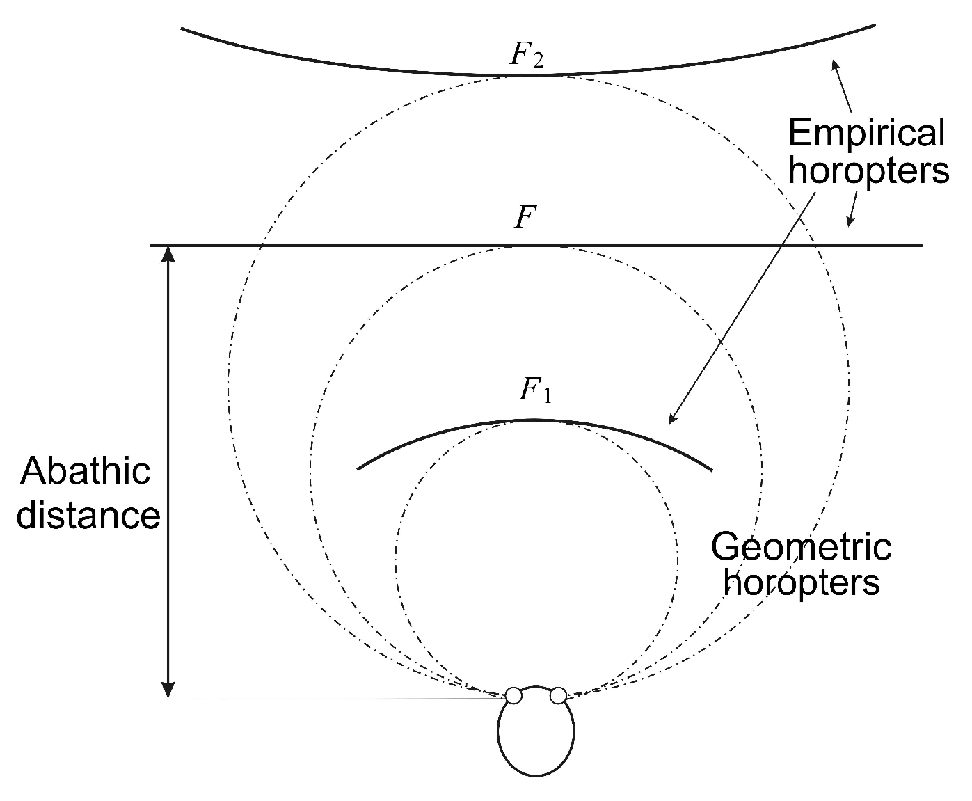
The importance of the eyes’ asymmetry follows from two facts. The first is well-known: the empirical longitudinal horopter deviates from the circular curves that form the geometric horopters. This so-called Hering–Hillebrand horopter deviation, shown in Figure 4, can be explained by asymmetry in the spatial positions of the corresponding elements in the two eyes. Two retinal elements, each one in a different eye, are corresponding if they invoke a single percept when stimulated. The second fact is the claim recently made in [44] that the natural crystalline lens tilt and decentration in humans is inclined to compensate for various types of aberration.
6. The Asymmetric Conformal Camera
To model the eye with both the tilt and decentration of the natural crystalline lens, we present in this section the asymmetric conformal camera. Although the optical axis should best approximate the lost symmetry in the alignment of the eye’s components, we assume that this axis is the line passing through the nodal point and the spherical eyeball’s rotation center.
The modified conformal camera is obtained by rotating the image plane about the -axis by the angle β and then translating the origin by , as shown in Figure 5. We refer to Figure 5 for the notation used in the remaining part of the paper. The immediate requirement is that the visual axis passing through the nodal point and point forms the angle with the optical axis.
However, because the nodal point is identified with the ‘north pole’ of the stereographic projection, the point , we place the nodal point 1 cm from the eye rotation center to simplify the discussion. This discrepancy with the physiological distance of 0.6 cm can be easily corrected. The angles and β give the fovea an asymmetric displacement of mm and the lens decentration .
The points on the image plane have coordinates relative to the plane origin . The projection of the space point on the tilted image plane with the ‘foveal’ center at can be expressed in terms of the projection z on the original image plane, allowing us to find the transformation between image planes. To this end, we note that .
Then, from the right triangles and , we get:
and:
Solving those last two formulas for and , and taking the difference, we obtain:
Next, from the right triangle , we have:
Introducing (20) to (19), we obtain:
which can be expressed by the following linear fractional action:
We call the matrix in (21) by , so that . If and , then shows that:
We have just derived the conjugate map of g by ,
which satisfies:
and:
The map (22) is the inner automorphism of the group . This inner automorphism maps the group of image projective transformations onto itself by using the image projective transformation that represents the camera’s asymmetry.
Since g and have the same algebraic properties by (23) and (24), they behave geometrically in the same way. For instance, the -transformation discussed in Section 1, which gives the image transformation from the conformal camera gaze change, is preserved under the conjugation because . Thus, we can work with the asymmetric conformal camera as we did with the standard conformal camera.
To this end, given the image intensity function in the standard conformal camera, we define the image intensity function:
on the image plane as follows: Then,
The relation between g and can be expressed in the following commutative diagram:
where the transformation can be considered a coordinate transformation. Then, the conjugate has the form corresponding to base changes in linear algebra. To see this, we let a linear map be represented by matrices M and N in two different bases. Then, , where P is the base change matrix.
The result of tilting and translating the image plane does not affect the conformal camera’s geometric and computational frameworks; this can be phrased as putting ‘conformal glasses’ on the camera.
7. Discussion: Modeling Empirical Horopters
Two points, each in one of the two eyes’ retinas, are considered corresponding if they give the same perceived visual direction. The circular shape of the geometric horopter is the consequence of a simple geometric assumption on corresponding points: two retinal points, onto which a non-fixated point in space is projected through each of the two nodal points, are corresponding if the angles subtended at the two eyes with fixation lines are equal.
If one relaxes this assumption by assuming that corresponding points in the temporal direction from the center of the fovea towards the periphery are compressed as compared with corresponding points in the nasal direction, the geometric horizontal horopter curves are no longer circular; see Figure 2.16 in [45].
The asymmetric conformal camera is defined by rotating the image plane by the angle β about the eye’s axis, the vertical axis to the horizontal visual plane and translating the plane origin by in the temporal direction (cf. Figure 5). In doing this, we demand that the angle between the fixation axis passing through the nodal point and point and the optical axis passing through the nodal point and spherical eyeball center of rotation is the angle . Here, is the stereographic projection of the fovea center f.
Now, a simple geometric fact follows: when equally-spaced points on the rotated image plane are projected into the sphere with the nodal point as the center of projection, their images on the sphere are compressed in the temporal direction from f, as compared with the nasal direction.
In this section, we study the horizontal horopter curves of the stereo system with asymmetric conformal cameras by back projecting the pairs of corresponding points from the uniformly-distributed points on the camera’s image plane to the object space. From [13], we expected that the horopters would be approximated by conics. To test this, we choose six points for each fixation: five points to give a unique conic curve and the sixth point to verify that this is indeed the horopter conic. One of these six points is the fixation point that is always on the horopter. Further, the nodal points and the point that does not project to the image plane, projecting instead to ∞, are taken as the points on the horopter, except for when the horopter is a straight line. When the horopter is a straight line, we need only three points.
To do this, we fix the camera’s parameters as follows. The abathic distance is the fixation point’s distance when the horopter is a straight line; see Figure 4. This occurs when the fixation point of the two eye models provides two image planes that are perpendicular to the head axis. This orientation of the eyes with the abathic distance at the fixation point is shown in Figure 5 if this figure is completed by adding the right eye as the reflection of the left eye about the head axis . Then, the abathic distance for the eye radius of 1 cm, with a given α, β and the ocular separation a, can be easily expressed as:
We use in (25) the physiologically-accurate values of and cm. Then, assuming the values of β in the range we find, using (25), the observed abathic distance values in humans in the range with an average value of cm. The assumed values of the angle β are in the range of the crystalline lens tilt’s angle, as measured in healthy human eyes [42].
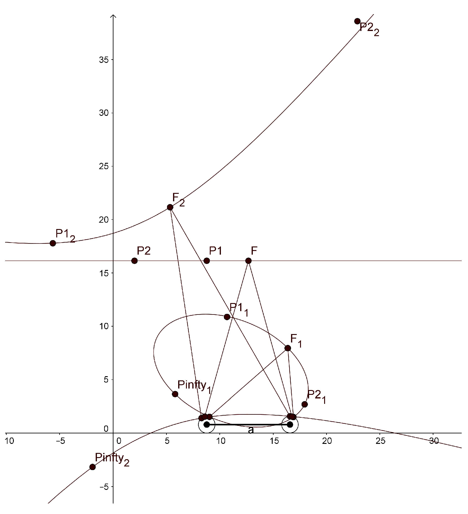
In the simulation with GeoGebra, we use different values for our parameters than those that would be used in the human binocular system. In order to display horopters with three different shapes, ellipse, straight line and hyperbola, in one graphical window output, we take the eye radius of 7.9 mm, the interocular distance of 78 mm, and . The graphs of the horopters obtained in GeoGebra are shown in Figure 6. The fixation points are given in the caption of this figure.
We note that the hyperbola has two branches, one passing through the fixation point and the other passing through the nodal points. GeoGebra also computed the conics’ equations:
the ellipse:
the line:
and the hyperbola:
The main purpose of the simulation with GeoGebra is to study qualitatively the shape of the horizontal horopters for the proposed binocular model to see how they are related to the empirical horopters. As we demonstrated before, our binocular model accounts for the typical characteristics of the human binocular system, such as the shape of horopter curves and the abathic distance. Most notably, the simulation with GeoGebra shows that the horopters given by the stereo system with eyes modeled by the asymmetric conformal cameras are well approximated by conical curves. It was proposed by Ogle in [13] that primates’ empirical horopters should be approximated by such conics.
8. Conclusions
The first part of the paper reviewed the conformal camera’s geometric analysis developed by the author in the group-theoretic framework [1,2,3]. We identified the semisimple group as the group of image transformations during the conformal camera’s gaze rotations. This group is the double cover of , the group that gives both the complex structure on the Riemann sphere and the one-dimensional complex geometry. This duality synthesizes the analytic and geometric structures.
Representation theory on semisimple groups, one of the greatest achievements of 20th century mathematics, allows the conformal camera to possess its own Fourier analysis. The projective Fourier transform was constructed by restricting Fourier analysis on the group to the image plane of the conformal camera. The image representation in terms of the discrete projective Fourier transform can be efficiently computed by a fast Fourier transform algorithm in the log-polar coordinates. These coordinates approximate the retino-cortical maps of the visual pathways. This means that the projective Fourier transform is well adapted to both image transformations produced by the conformal camera’s gaze change and to the correspondingly updated log-polar maps.
The first part of the paper was concluded with a discussion of the conformal camera’s relevance to the computational aspects of anthropomorphic vision. First, we discussed the relevance of imaging with the conformal camera to early and intermediate-level vision. Then, we compared the conformal camera model of retinotopy with the accepted Schwartz model and pointed out the conformal camera’s advantages in biologically-mediated image processing. We also discussed numerical implementation of the discrete projective Fourier transform. In this implementation, the log-polar image contained 100-times less pixels than the original image, comparable to the ratio of 125 million photoreceptors sampling incoming visual information to 1.5 million of ganglion cell axons carrying the output from the eye to the brain. Finally, we briefly reviewed image processing for stability during the conformal camera tracking and saccadic movements.
The model with the conformal camera was developed to process visual information in an anthropomorphic camera head mounted on a moving platform replicating human eye movements. It was demonstrated in the author’s previous studies that this model is capable of supporting the stability of foveate vision when the environment is explored with about four saccadic eye movements per second and when the eye executes smooth pursuit eye movements. Previously, this model only considered aspects of monocular vision.
In the second part of the paper, binocular vision was reviewed and the stereo extension of the conformal camera’s group-theoretic framework was presented. We did this for the eye model that includes the asymmetrically-displaced fovea on the retina and the tilted and decentered natural crystalline lens. We concluded this part showing, with a numerical simulation, that the resultant horopters are conics that well approximate the empirical horopters.
The geometry of the conical horopters in the stereo system with asymmetric conformal cameras requires further study. In the near future, the spatial orientation and shape of the conic curves need to be derived in terms of the perceived direction and the parameters of asymmetry. This will allow the development of disparity maps for the stereo system with asymmetric conformal cameras.
Acknowledgments
The author thanks the reviewers for helpful comments. The research presented in this paper was supported in part by NSF Grant CCR-9901957.
Conflicts of Interest
The author declares no conflict of interest.
Abbreviations
The following abbreviations are used in this manuscript:
| PFT | projective Fourier transform |
| DPFT | discrete projective Fourier transform |
| FFT | fast Fourier transform |
| SC | superior colliculus |
| LGN | lateral geniculate nucleus |
| V1 | primary visual cortex |
| ECT | exponential chirp transform |
References
- Turski, J. Projective Fourier analysis for patterns. Pattern Recognit. 2000, 33, 2033–2043. [Google Scholar] [CrossRef]
- Turski, J. Geometric Fourier Analysis of the Conformal Camera for Active Vision. SIAM Rev. 2004, 46, 230–255. [Google Scholar] [CrossRef]
- Turski, J. Geometric Fourier Analysis for Computational Vision. J. Fourier Anal. Appl. 2005, 11, 1–23. [Google Scholar] [CrossRef]
- Turski, J. Robotic Vision with the Conformal Camera: Modeling Perisaccadic Perception. J. Robot. 2010. [Google Scholar] [CrossRef]
- Turski, J. Imaging with the Conformal Camera. In Proc IPCVIPR; CSREA Press: Las Vegas, NV, USA, 2012; Volume 2, pp. 1–7. [Google Scholar]
- Turski, J. Modeling of Active Vision During Smooth Pursuit of a Robotic Eye. Electron. Imaging 2016, 10, 1–8. [Google Scholar]
- Jones, G.; Singerman, D. Complex Functions; Cambridge University Press: Cambridge, UK, 1987. [Google Scholar]
- Henle, M. Modern Geometries. The Analytical Approach; Prentice Hall: Upper Saddle River, NJ, USA, 1997. [Google Scholar]
- Berger, M. Geometry I; Springer: New York, NY, USA, 1987. [Google Scholar]
- Knapp, A.W. Representation Theory of Semisimple Groups: An Overview Based on Examples; Princeton University Press: Princeton, NJ, USA, 1986. [Google Scholar]
- Kaas, J.H. Topographic Maps are Fundamental to Sensory Processing. Brain Res. Bull. 1997, 44, 107–112. [Google Scholar] [CrossRef]
- Larson, A.M.; Loschky, L.C. The contributions of central versus peripheral vision to scene gist recognition. J. Vis. 2009, 9, 1–16. [Google Scholar] [CrossRef] [PubMed]
- Ogle, K.N. Analytical treatment of the longitudinal horopter. J. Opt. Soc. Am. 1932, 22, 665–728. [Google Scholar] [CrossRef]
- Bonmassar, G.; Schwartz, E.L. Space-variant Fourier analysis: The Exponential Chirp transform. IEEE Trans. Pattern Anal. 1997, 19, 1080–1089. [Google Scholar] [CrossRef]
- Schwartz, E.L. Computational anatomy and functional architecture of striate cortex. Vis. Res. 1980, 20, 645–669. [Google Scholar] [CrossRef]
- Balasuriya, L.S.; Siebert, J.P. An artificial retina with a selforganized retina receptive field tessellation. In Proceedings of the AISB 2003 Symposium: Biologically Inspired Machine Vison, Theory and Applications, Aberystwyth, UK, 7–11 April 2003; pp. 34–42.
- Bulduc, M.; Levine, M.D. A review of bilogically motivated space-variant data reduction models for robotic vision. Comput. Vis. Image Underst. 1998, 689, 170–184. [Google Scholar] [CrossRef]
- You, S.; Tan, R.T.; Kawakami, R.; Mukaigawa, Y.; Ikeuch, K. Waterdrops Stereo. Available online: https://arxiv.org/pdf/1604.00730.pdf (accessed on 4 April 2016).
- Taguchi, Y.; Agrawal, A.; Veeraraghavan, A.; Ramalingam, S.; Raskar, R. Axial-Cones: Modeling Spherical Catadioptric Cameras for Wide-Angle Light Field Rendering. ACM Trans. Graph. 2010, 29. [Google Scholar] [CrossRef]
- Needham, T. Visual Complex Analysis; Oxford University Press: New York, NY, USA, 2002. [Google Scholar]
- Altmann, S.L. Rotations, Quaternions and Double Groups; Oxford University Press: Oxford, UK; New York, NY, USA, 1986. [Google Scholar]
- Sally, P.J., Jr. Harmonic analysis and group representations. In Studies in Harmonic Analysis; Ash, J.M., Ed.; Mathematical Association of America: Washington, DC, USA, 1976; Volume 13, pp. 224–256. [Google Scholar]
- Herb, R.A. An Elementary Introduction to Harish-Chandra’s Work. In Mathematical Legacy of Harish-Chandra—A Celebration of Representation Theory and Harmonic Analysis; Doran, R.S., Varadarajan, V.S., Eds.; AMS: Providence, RI, USA, 2000; Volume 68, pp. 59–75. [Google Scholar]
- Shapley, R. Early vision is early in time. Neuron 2007, 56, 755–756. [Google Scholar] [CrossRef] [PubMed]
- Roelfsema, P.R.; Tolboom, M.; Khayat, P.S. Different Processing Phases for Features, Figures, and Selective Attention in the Primary Visual Cortex. Neuron 2007, 56, 785–792. [Google Scholar] [CrossRef] [PubMed]
- Blum, H. Biological shape and visual science. J. Theor. Biol. 1973, 38, 205–287. [Google Scholar] [CrossRef]
- Hoffman, D.D.; Richards, W.A. Parts of recognition. Cognition 1984, 18, 65–96. [Google Scholar] [CrossRef]
- Kovacs, I.; Julesz, B. Perceptual sensitivity maps within globally defined visual shapes. Nature 1994, 370, 644–646. [Google Scholar] [CrossRef] [PubMed]
- Engel, S.A.; Glover, G.H.; Wendell, B.A. Retinotopic organization in human visual cortex and the spatial precision of MRI. Cerabral Cortex. 1997, 7, 181–192. [Google Scholar] [CrossRef]
- Tabareau, N.; Bennequin, N.D.; Berthoz, A.; Slotine, J.-J. Geometry of the superior colliculic mapping and efficient oculomotor computation. Biol. Cybern. 2007, 97, 279–292. [Google Scholar] [CrossRef] [PubMed]
- Shapiro, A.; Lu, Z.-L.; Huang, C.-B.; Knight, E.; Ennis, R. Transitions between Central and Peripheral Vision Create Spatial/Temporal Distortions: A Hypothesis Concerning the Perceived Break of the Curveball. PLoS ONE 2010, 5. [Google Scholar] [CrossRef] [PubMed]
- Xing, J.; Heeger, D.J. Center-surround interaction in foveal and peripheral vision. Vis. Res. 2000, 40, 3065–3072. [Google Scholar] [CrossRef]
- Newsome, W.T.; Wurtz, R.H.; Komatsu, H. Relation of cortical areas MT and MST to pursuit eye movements. II. Differentiation of retinal from extraretinal imputes. J. Neurophysiol. 1988, 60, 604–620. [Google Scholar] [PubMed]
- Sommer, M.A.; Wurtz, R.H. A pathway in primate brain for internal monitoring of movements. Science 2002, 296, 1480–1482. [Google Scholar] [PubMed]
- Hall, N.J.; Colby, C.L. Remapping for visual stability. Philos. Trans. R. Soc. 2010, 366, 528–539. [Google Scholar] [CrossRef] [PubMed]
- VanRullen, R. A simple translation in cortical log-coordinates may account for the pattern of saccadic localization errors. Biol. Cybern. 2004, 91, 131–137. [Google Scholar] [CrossRef] [PubMed]
- Ross, J.; Morrone, M.C.; Goldberg, M.E.; Burr, D.C. Changes in visual perception at the time of saccades. Trend Neurosci. 2001, 24, 113–121. [Google Scholar] [CrossRef]
- Marr, D. Vision; Freeman: New York, NY, USA, 1985. [Google Scholar]
- Turski, J. On Binocular Vision: The Geometric Horopter and Cyclopean Eye. Vis. Res. 2016, 119, 73–81. [Google Scholar] [CrossRef] [PubMed]
- Wilcox, L.M.; Harris, J.M. Fundamentals of stereopsis. In Encyclopedia of the Eye; Dartt, D.A., Besharse, J.C., Dana, R., Eds.; Academic Press: New York, NY, USA, 2007; Volume 2, pp. 164–171. [Google Scholar]
- Ponce, C.R.; Born, R.T. Stereopsis. Curr. Biol. 2008, 18, R845–R850. [Google Scholar] [CrossRef] [PubMed]
- Chang, Y.; Wu, H.-M.; Lin, Y.-F. The axial misalignment between ocular lens and cornea observed by MRI (I)—At fixed accommodative state. Vis. Res. 2007, 47, 71–84. [Google Scholar] [CrossRef] [PubMed]
- Mester, U.; Tand, S.; Kaymak, H. Decentration and tilt of a single-piece aspheric intraocular lens compared with the lens position in young phakic eyes. J. Cataract Refract. Surg. 2009, 35, 485–490. [Google Scholar] [CrossRef] [PubMed]
- Artal, P.; Guirao, A.; Berrio, E.; Williams, D.R. Compensation of corneal aberrations by the internal optics in the human eye. J. Vis. 2001, 1, 1–8. [Google Scholar] [CrossRef] [PubMed]
- Howard, I.P.; Rogers, B.J. Binocular Vision and Stereopsis; University Press Scholarship Online: Oxford, UK, 2008. [Google Scholar]
Figure 1.
The conformal camera as the eye model. The points in the object space are centrally projected into the sphere. The sphere and the center of projection N represent the eye’s retina and nodal point. The ‘image’ entity is given by stereographic projection σ from the sphere to the plane . Because σ is conformal and maps circles to circles (see the text), it preserves the ‘retinal illuminance’, that is the pixels. This image representation is appropriate for efficient computational processing.
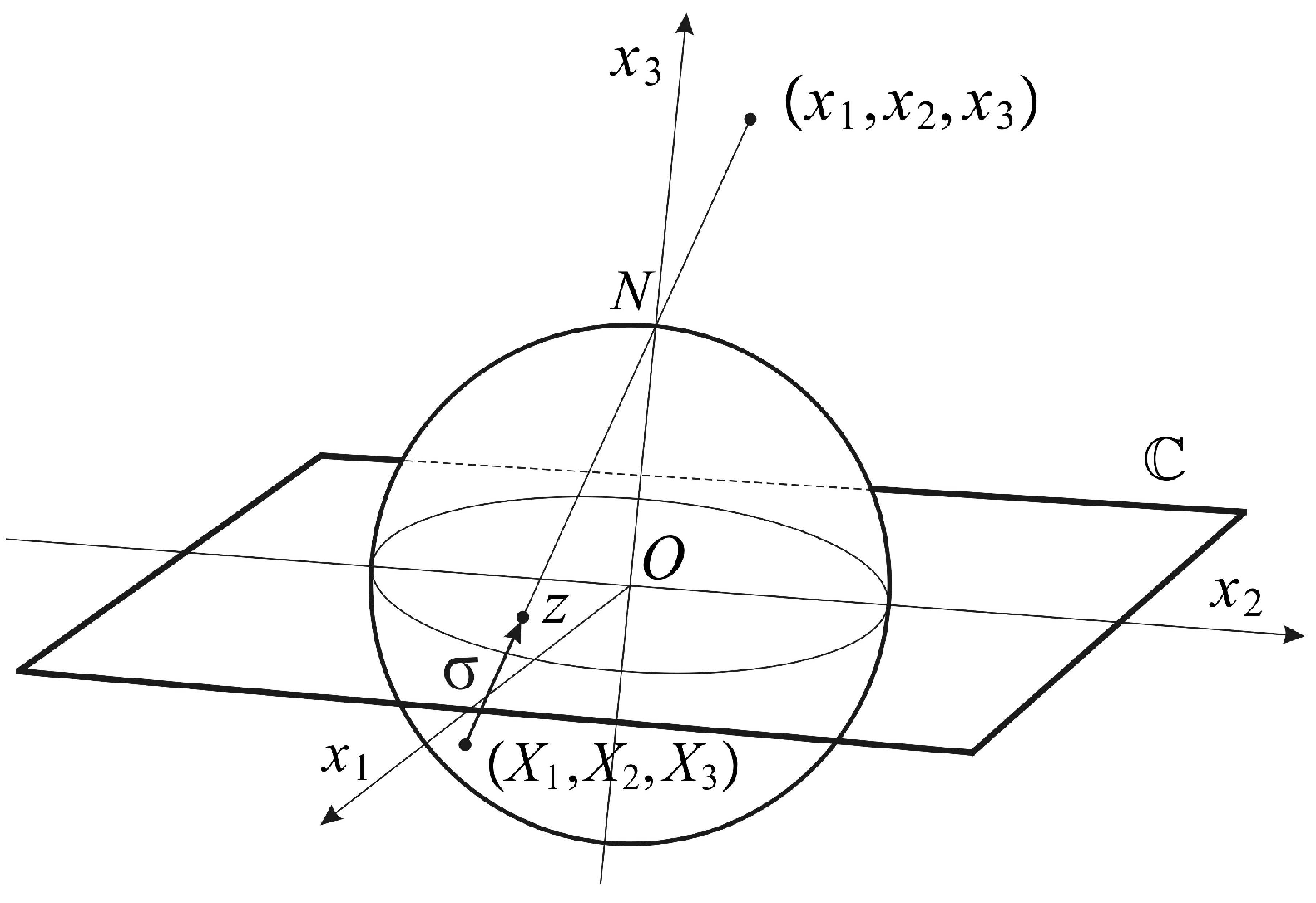
Figure 2.
(a) When the camera gaze is rotated by ϕ, the image projective transformation is given here in the rotated image plane by the g-transformation that results from the composition of two basic image transformations. The first involves the image that is translated by the vector () and projected back into the image plane. The second transformation is given in terms of the image projected into the sphere, rotated by , and projected back into the image plane. The image transformation adds the conformal distortions, schematically shown by the transformed image’s back projection into the plane containing the planar object. (b) The camera and scene are shown in the view seen when looking from above. Here, the sequence of transformations explains the image projective transformation.
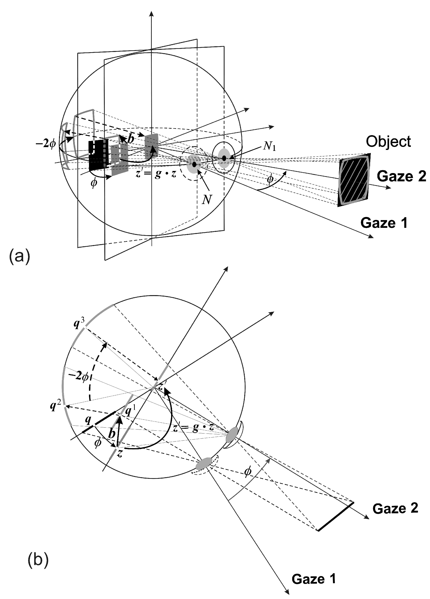
Figure 3.
When the camera gaze is rotated by ϕ, the image projective transformation is given by the g-transformation where is the result of the composition of the line segment relative movements. Since the gaze rotation induces the nodal point translation by , the object relative movements in the scene are composed of the translation by corresponding to the translation of the image by (i.e., the h-transformation) and the rotation by corresponding to the sphere rotation by (i.e., the k-transformation).
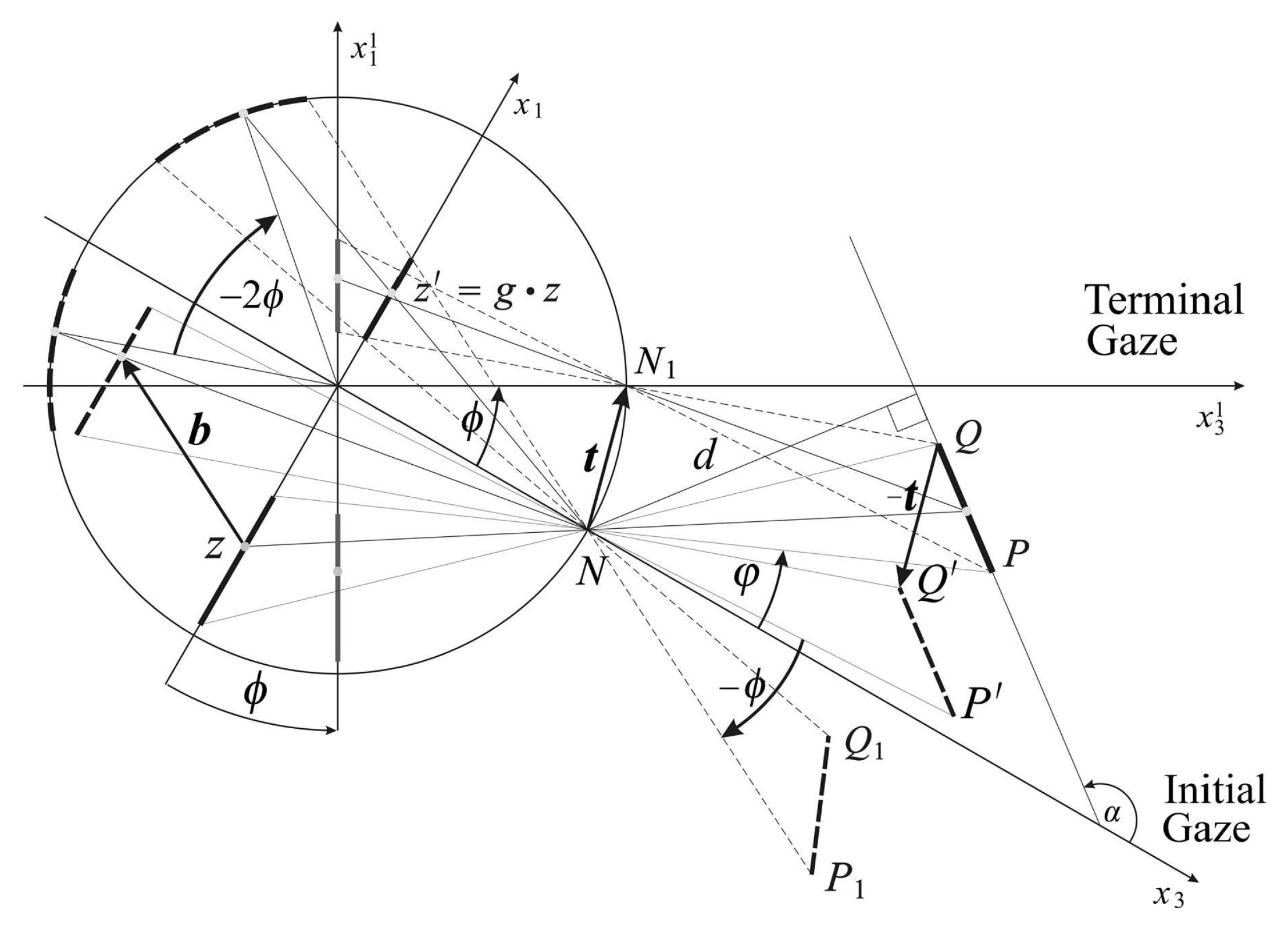
Figure 4.
Empirical longitudinal horopters are shown schematically for symmetric convergence points. Abathic distance is defined here as the distance from the line connecting the eye centers to the fixation point F at which the horopter is a straight line.
Figure 4.
Empirical longitudinal horopters are shown schematically for symmetric convergence points. Abathic distance is defined here as the distance from the line connecting the eye centers to the fixation point F at which the horopter is a straight line.

Figure 5.
The eye model with an asymmetrically-displaced fovea and a tilted and decentered lens outlined with thin (1 pt) curves. The asymmetric conformal camera is outlined with thick (2 pt) curves. The stereo system is obtained if the left camera is reflected in the head axis . Each camera’s image plane, shown here for the left eye, is perpendicular to the head axis, such that the horopter curve is a straight line passing through the fixation point F at the abathic distance from origin O.

Figure 6.
The graphs of the three horizontal horopters, the ellipse for fixation , the straight line for fixation and the hyperbola for fixation , with coordinates given in millimeters. The eye radius is 7.9 mm; the interocular distance is 78.0 mm, and . For each of the fixations , , the six points were obtained by back projecting the corresponding points. These six points included the fixation point, the two nodal points, the point that projects to ∞ and two additional points, and . Five of these points were used to obtain the conics, and the sixth point was used for the verification. The straight-line horopter is for the fixation point at the abathic distance and is given by three points, F, and .
© 2016 by the author; licensee MDPI, Basel, Switzerland. This article is an open access article distributed under the terms and conditions of the Creative Commons Attribution (CC-BY) license (http://creativecommons.org/licenses/by/4.0/).
Share and Cite
MDPI and ACS Style
Turski, J. The Conformal Camera in Modeling Active Binocular Vision. Symmetry 2016, 8, 88. https://doi.org/10.3390/sym8090088
AMA Style
Turski J. The Conformal Camera in Modeling Active Binocular Vision. Symmetry. 2016; 8(9):88. https://doi.org/10.3390/sym8090088
Chicago/Turabian StyleTurski, Jacek. 2016. "The Conformal Camera in Modeling Active Binocular Vision" Symmetry 8, no. 9: 88. https://doi.org/10.3390/sym8090088
Note that from the first issue of 2016, this journal uses article numbers instead of page numbers. See further details here.