
Modeling Bottom-Up Visual Attention Using Dihedral Group D4 †


Department of Engineering & Safety (IIS-IVT), UiT-The Arctic University of Norway, Tromsø-9037, Norway
†
This paper is an extended version of my paper published in 11th International Symposium on Visual Computing (ISVC 2015).
Symmetry 2016, 8(8), 79; https://doi.org/10.3390/sym8080079
Submission received: 27 April 2016
/
Revised: 19 July 2016
/
Accepted: 9 August 2016
/
Published: 15 August 2016
(This article belongs to the Special Issue Symmetry in Vision)
Abstract
:In this paper, first, we briefly describe the dihedral group that serves as the basis for calculating saliency in our proposed model. Second, our saliency model makes two major changes in a latest state-of-the-art model known as group-based asymmetry. First, based on the properties of the dihedral group , we simplify the asymmetry calculations associated with the measurement of saliency. This results is an algorithm that reduces the number of calculations by at least half that makes it the fastest among the six best algorithms used in this research article. Second, in order to maximize the information across different chromatic and multi-resolution features, the color image space is de-correlated. We evaluate our algorithm against 10 state-of-the-art saliency models. Our results show that by using optimal parameters for a given dataset, our proposed model can outperform the best saliency algorithm in the literature. However, as the differences among the (few) best saliency models are small, we would like to suggest that our proposed model is among the best and the fastest among the best. Finally, as a part of future work, we suggest that our proposed approach on saliency can be extended to include three-dimensional image data.
1. Introduction
While searching for a person on a busy street, we look at people while neglecting other aspects of the scene, such as road signs, buildings and cars. However, in the absence of the given task, we would pay attention to different features of the same scene. In the literature [1], it is described as a combination of two different mechanisms: top-down and bottom-up.
Top-down pertains to how a target object is defined or described in the scene; for instance, while searching for a person, we would start by selecting all people in the scene as likely candidates and disregard the candidates that do not match the features of the target person until the correct person is found. To model this, we need a description of the scene in terms of all of the objects, and the unique features associated with each object, such that the uniqueness of the features can be used for distinguishing similar objects from one another. Given the sheer number of man-made and natural objects in our daily lives and the ambiguity associated with the definition of an object itself makes the modeling of top-down mechanisms perplexing. To this end, recent attempts have been made by [2,3] using machine learning-based methods.
Bottom-up (also known as visual saliency) mechanisms are associated with the attributes of a scene that draw our attention to a particular location. These low-level image attributes include: motion, color, contrast and brightness [4]. Bottom-up mechanisms are involuntary and faster compared to top-down ones [1]. For instance, a red object among green objects and an object placed horizontally among vertical objects are some stimuli that would automatically capture our attention in the environment. Owing to the limited number of low-level image attributes, modeling visual saliency is relatively less complex.
In the past two decades, modeling visual saliency has generated much interest in the research community. In addition to contributing towards the understanding of human vision, it has also paved the way for a number of computer and machine vision applications. These applications include: image and video compression [5,6,7,8], robot localization [9,10], image retrieval [11], image and video quality assessment [12,13], dynamic lighting [14], advertisement [15], artistic image rendering [16] and human-robot interaction [17,18]. In salient object detection, the applications include: target detection [19], image segmentation [20,21] and image resizing [22,23].
In a recent study by Alsam et al. [24,25], it was proposed that asymmetry can be used as a measure of saliency. In order to calculate the asymmetry of an image region, the authors used dihedral group , which is the symmetry group of the square. consists of eight group elements, namely rotation by 0, 90, 180 and 270 degrees and reflection about the horizontal, vertical and two diagonal axes. The saliency maps obtained from their algorithm show good correspondence with the saliency maps calculated from the classic visual saliency model by Itti et al. [26].
Inspired by the fact that bottom-up calculations are fast, in this paper, we use the symmetries present in the dihedral group to make the calculations associated with the group elements simpler and faster to implement. In doing so, we modify the saliency model proposed by Alsam et al. [24,25]. For details, please see Section 3.
Next, we are motivated by the study by Garcia-Diaz et al. [27], which implies that in order to quantify distinct information in a scene, our visual system de-correlates its chromatic and multi-resolution features. Based on this, we perform the de-correlation of the input color image by calculating its principal components (details in Section 3.3).
2. Theory
A dihedral group is the group of symmetries of an n-sided regular polygon, i.e., all sides have the same length, and all angles are equal. has n rotational symmetries and n reflection symmetries. In other words, it has n axes of symmetry and 2n different symmetries [28]. For instance, the polygons for n = 3, 4, 5 and 6 and the associated reflection symmetries are shown in Figure 1. Here, we can see that when n is odd, each axis of symmetry connects the vertex with the midpoint of the opposite side. When n is even, there are n/2 symmetry axes connecting the midpoints of opposite sides and n/2 symmetry axes connecting opposite vertices.
A group is a set G together with a binary operation on its elements. This operation must behave such that:
- (i)
- G must be closed under , that is for every pair of elements in G, we must have that is again an element in G.
- (ii)
- The operation must be associative, that is for all elements in G, we must have that:
- (iii)
- There is an element e in G, called the identity element, such that for all , we have that:
- (iv)
- For every element g in G, there is an element in G, called the inverse of g, such that:
The Group
In this paper, we are interested in , the symmetry group of the square. The ease of computational complexity associated with dividing an image grid into square regions and the fact that the group has shown promising results in various computer vision applications [29,30,31,32,33] motivated us to use this group for our proposed algorithm.
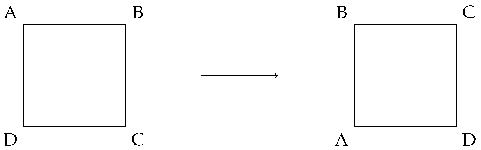
The group has eight elements, four rotational symmetries and four reflection symmetries. The rotations are 0, 90, 180and 270, and the reflections are defined along the four axes shown in Figure 1. We refer to these elements as . Note that the identity element is rotation by 0and that for each element, there is another element that has the opposite effect on the square, as required in the definition of a group. The group operation is the composition of two such transformations. As an example of one of the group elements, consider Figure 2, where we demonstrate rotation by 90counterclockwise on a square with labeled corners.
3. Method
3.1. Background
Alsam et al. [24,25] proposed a saliency model that uses asymmetry as a measure of saliency. In order to calculate saliency, the input image is decomposed into non-overlapping square blocks (as shown at the top-left in Figure 3), and for each block, the absolute difference between the block itself and the result of the group elements acting on the block is calculated. As shown at the bottom-right in Figure 3, the asymmetry values of the square blocks pertaining to uniform regions are close to zero. The sum of the absolute differences (also known as the norm) for each block is used as a measure of the asymmetry for the block. The asymmetry values for all of the blocks are then collected in an image matrix and scaled up to the size of the original image using bilinear interpolation. In order to capture both the local and the global salient details in an image, three different image resolutions are used. All maps are combined linearly to get a single saliency map.
In their algorithm, the asymmetry of a square region is calculated as follows: M (i.e., the square block) is defined as an -matrix and as one of the eight group elements of . The eight elements are the rotations along 0, 90, 180and 270and the reflections along the horizontal, vertical and two diagonal axes of the square. As an example, the eight group transformations pertaining to a square block of the image are shown in Figure 3. Asymmetry of M by is denoted by to be,
where represents the norm. Instead of calculating asymmetry values associated with each group element and followed by their sum, we propose that the algorithm can run faster if the calculations in Equation (1) are made simpler. For this, we propose a fast implementation of these operations pertaining to the group elements.
3.2. Fast Implementation of the Group Operations
Let us assume M as a 4 by 4 matrix,
![Symmetry 08 00079 i001]()

The asymmetry of the matrix M is measured as the sum of the absolute differences of the different permutations of the matrix entries pertaining to the group elements and the original. The total number of such differences is determined to be 40. As the calculations associated with absolute differences are repeated for the rotation and reflection elements of the dihedral group , our objective is to find the factors associated with these repeated differences.
For our calculations, we divide the set of matrix entries into two computational categories: the diagonal entries (highlighted in yellow) and the rest of the entries of M. Please note that these calculations can be generalized to any matrix of size n by n, given that n is even.
For the rest of the entries, first, we can look at . This element will only be possible if we flip the matrix about the vertical axis. This will result in two parts in the sum, and , giving a factor 2. Here, a and b represent a reflection symmetric pair, and all other reflection symmetric pairs will behave in the same way. Now, let us focus on . This represents a rotational symmetric pair. Rotating the matrix counterclockwise will move d onto the position of a giving a part in the sum. Rotating clockwise gives us . As these differences are not plausible in any other way, this gives us a factor of 2. All other rotational symmetric pairs will behave in the same way. This means that the asymmetry for the rest of the entries can be calculated as follows:
For the diagonal entries, we can see that they exhibit both rotation and reflection symmetries. For instance, we can move β to the place of α and α to β with one reflection and two rotations. This gives us a factor of 4. The asymmetry of one set of diagonal entries can be calculated as follows:
The asymmetry for both diagonal entries and the rest is represented as,
As shown in Equation (4), the asymmetry calculations associated with the matrix M are reduced to a quarter for the diagonal entries and one-half for the rest of the entries. This makes the proposed algorithm at least twice as fast.
3.3. De-Correlation of Color Image Channels
De-correlation of color image channels is done as follows: First, using bilinear interpolation, we create three resolutions (original, half and quarter) of the RGB color image. In order to collect all of the information in a matrix, the (half and one-quarter) resolutions are rescaled to the size of original. This gives us a matrix I of size w by h by n, where w is the width of the original, h is the height and n is the number of channels ().
Second, by rearranging the matrix entries of I, we create a two-dimensional matrix A of size by n. We do normalization of A around the mean as,
where μ is the mean for each of the channels, and B is by n.
Third, we calculate the correlation matrix of B as,
where the size of C is n by n.
Fourth, the Eigen decomposition of a symmetric matrix is represented as,
where V is a square matrix whose columns are eigenvectors of C and D is the diagonal matrix whose diagonal entries are the corresponding eigenvalues.
Finally, the image channels are transformed into eigenvector space (also known as principal components) as:
where E is the transformed space matrix, which is rearranged to get back the de-correlated channels.
3.4. Implementation of the Algorithm
First, the input color image is rescaled to half the original resolution. Second, by using the de-correlation procedure described in Section 3.3 on the resulting image, we get 9 de-correlated multi-resolution and chromatic channels. Third, a fixed block size (e.g., 12) is selected, as discussed later in Section 4.6; this choice is governed by the dataset. If the rows and columns of the de-correlated channels are not divisible by the block size, then they are padded with neighboring information along the right and bottom corners. Finally, the saliency map is generated by using the procedure outlined in Section 3.2. The code is open source and is available at Matlab Central for the research community.
4. Comparing Different Saliency Models
The performance of visual saliency algorithms is usually judged by how well the two-dimensional saliency maps can predict the human eye fixations for a given image. Center-bias is a key factor that can influence the evaluation of saliency algorithms [34].
4.1. Center-Bias
While viewing images, observers tend to look at the center regions more as compared to peripheral regions. As a result of that, a majority of fixations fall at the image center. This effect is known as center-bias and is well documented in vision studies [35,36]. The two main reasons for this are: first, the tendency of photographers to place the objects at the center of the image; second, the viewing strategy employed by observers, i.e., to look at center locations more in order to acquire the most information about a scene [37]. The presence of center-bias in fixations makes it difficult to analyze the correspondence between the fixated regions and the salient image regions.
4.2. Shuffled Metric
The shuffled metric was proposed by Tatler et al. [35] and later used by Zhang et al. [38] to mitigate the effect of center-bias in fixations. The shuffled metric is a variant of [39], which is known as the area under the receiver operating characteristic curve. For a detailed description of , please see the study by Fawcett [39].
To calculate the shuffled metric for a given image and one observer, the locations fixated by the observer are associated with the positive class (in a manner similar to the regular metric); however, the locations for the negative class are selected randomly from the fixated locations of other unrelated images, such that they do not coincide with the locations from the positive class. Similar to the regular , the shuffled metric gives us a scalar value in the interval [0,1]. If the value is one then it indicates that the saliency model is perfect in predicting fixations. If shuffled , then it implies that the performance of the saliency model is not better than a random classifier or chance prediction.
4.3. Dataset
For the analysis, we used the eye tracking database from the study by Judd et al. [16]. The database consists of 1003 images selected randomly from different categories and different geographical locations. In the eye tracking experiment [16], these images were shown to fifteen different users under free viewing conditions for a period of 3 s each. In the database, a majority of the images are 1024 pixels in width and 768 pixels in height. These landscape images were specifically used in the evaluation.
4.4. Saliency Models
For our comparison, eleven state-of-the-art saliency models, namely, AIM by Bruce and Tsotsos [40], AWS by Garcia-Diaz et al. [27], Erdem by Erdem and Erdem [22], Hou by Hou and Zhang [41], Spec by Schauerte and Stiefelhagen [42], GBA by Alsam et al. [24,25], fast GBA proposed in this paper (, , ; for details, please see Section 4.6), GBVS by Harel et al. [43], Itti by Itti et al. [26], Judd by Judd et al. [16] and LG by Borji and Itti [44] are used. In line with the study by Borji et al. [45], two models are selected to provide a baseline for the evaluation. Gauss is defined as a two-dimensional Gaussian blob at the center of the image. Different radii of the Gaussian blob are tested, and the radius that corresponds best with human eye fixations is selected.
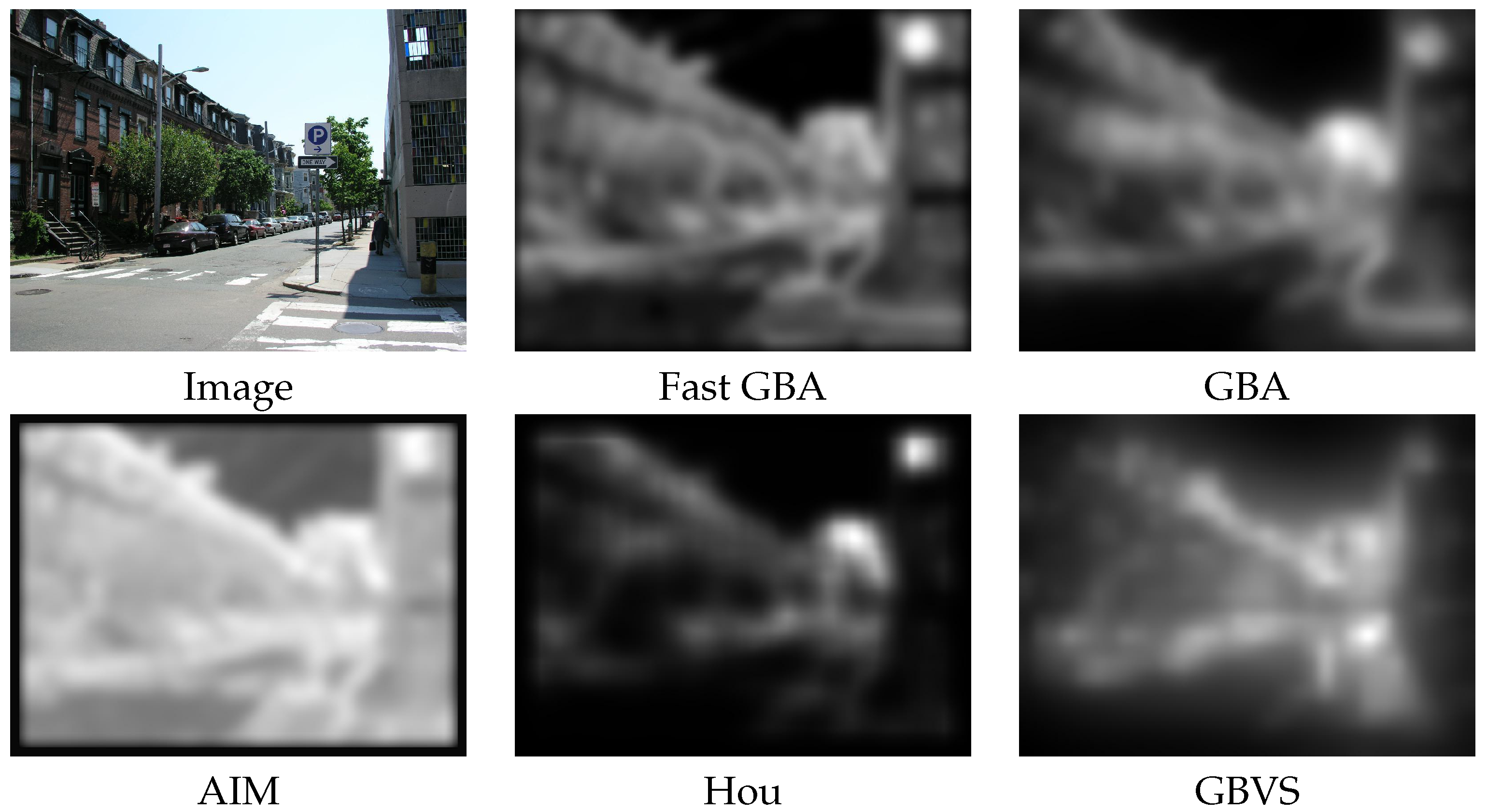
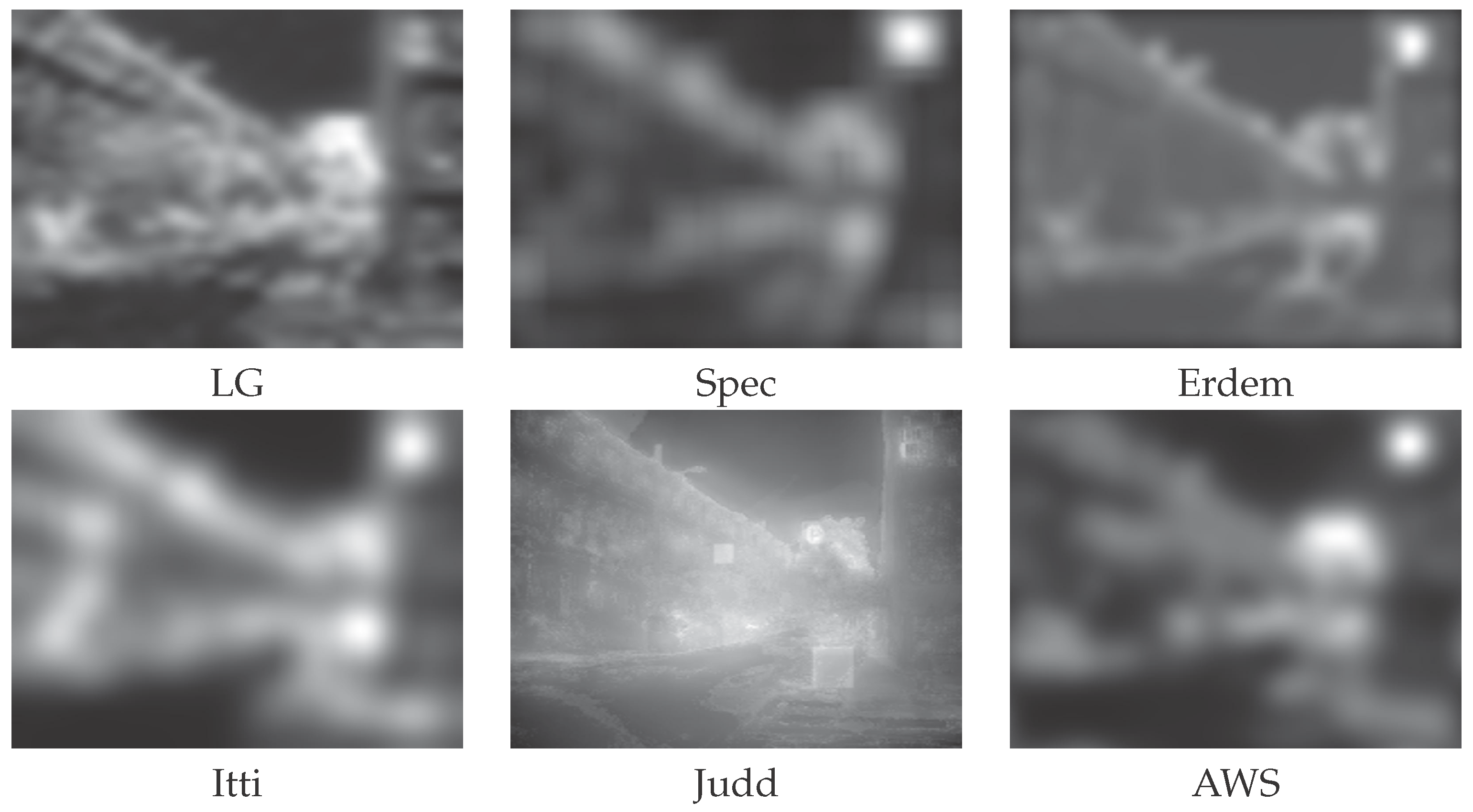
The IO model is based on the fact that an observer’s fixations can be predicted best by the fixations of other observers viewing the same image. In this model, the map for an observer is calculated as follows: first, the fixations corresponding to a given image from all of the observers except the one under consideration are averaged into a single two-dimensional map. Having done that, the fixations are spread by smoothing the map using a Gaussian filter. The IO model gives us an upper bound on the level of correspondence that is expected between the saliency models and the fixations. Figure 4 shows a test image and the associated saliency maps from different saliency algorithms.
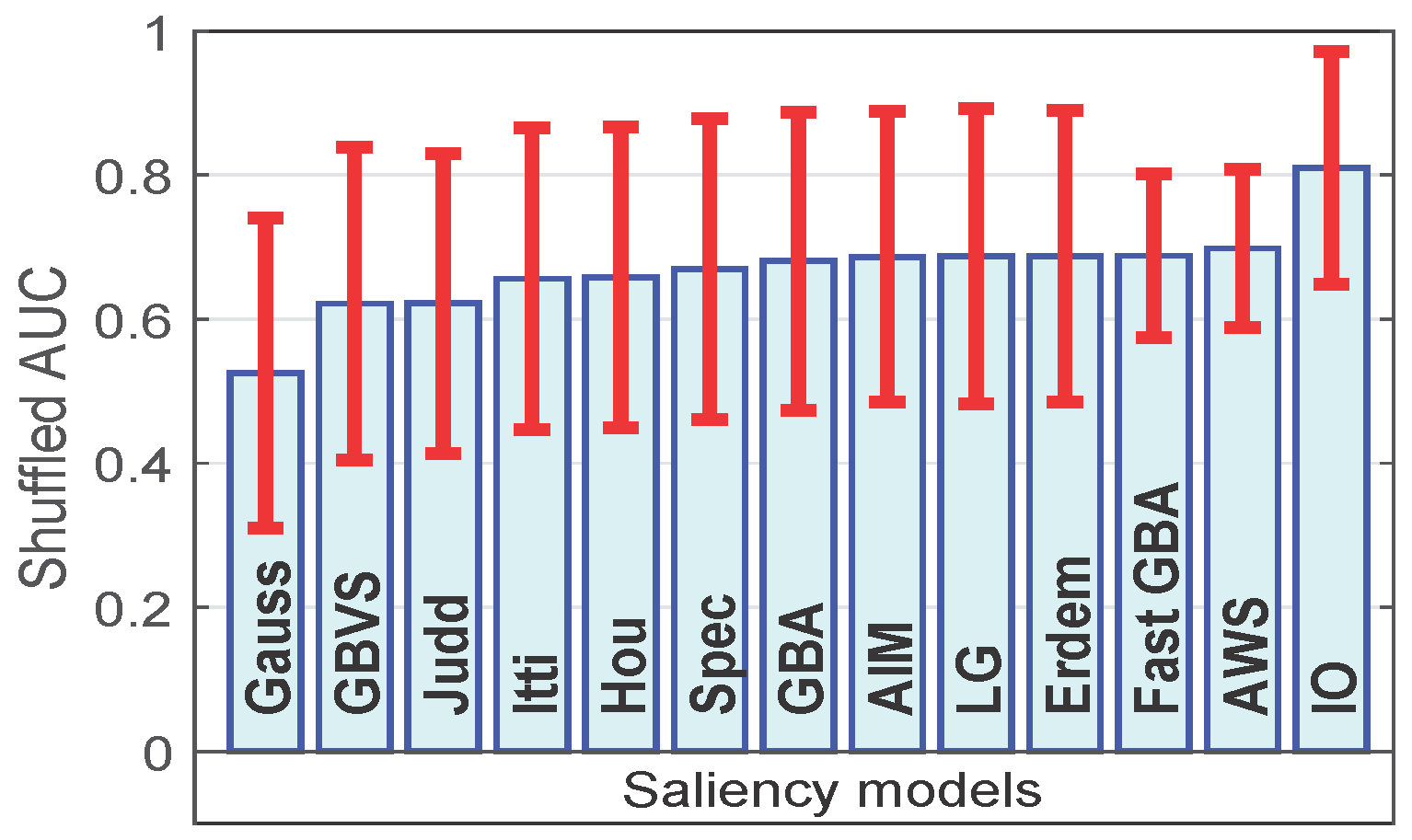
4.5. Ranking among the Saliency Models
We compare the ranking of saliency models using the shuffled metric. From the results in Figure 5, we note that, first, the Gauss model is ranked the worst indicating that the shuffled metric counters the effects associated with the center-bias. Second, the AWS model is ranked the best followed by the proposed fast GBA model. It is important to note that a majority of the state-of-the-art saliency models, such as Itti, Hou, Spec, GBA, fast GBA LG, Erdem, AIM and AWS, are quite close to each other in terms of their performance.
Next, we compare the average run times (for 463 landscape images) of the saliency models that rank at the same or better than Itti, i.e., the classic saliency model. For a better visualization, we use the natural logarithm of the average run times. For this, we used MATLAB R2015 on a 64-bit windows PC with a 3.16-GHz Intel processor and 4 GB RAM. From Figure 6, we observe that the algorithms Hou, and Spec are the fastest. However, among the top six algorithms, the proposed fast GBA model is the fastest. Furthermore, it shows that Fast GBA is nearly 31-times faster than the original GBA algorithm. It is important to note that the original GBA algorithm is crude in implementation, i.e., the eight group transformations are performed iteratively and kept in the memory. In the fast GBA model, reducing the computational complexity (by employing the steps mentioned in Section 3.2) also reduces the memory and software complexity of the proposed model, which is reflected in the results.
4.6. Optimizing the Proposed Fast GBA Model
The performance of the proposed model is influenced by the choice of parameters, such as block size, which depends on the size of an average image in the database used for testing. To find the optimal parameters for our algorithm, we use three variables: image scaling factor (which rescales the original image in order to reduce the number of calculations), block size b and number of resolutions (different resolutions to capture local and global details). For this analysis, we use (half size) and , b in the range [12, 50], and 1, 2 and 3. The results obtained by using the shuffled metric for the three variables are shown in the first row of Figure 7. The figure on the top-left shows the shuffled values for , with the red, green and blue lines depicting as 1, 2 and 3, respectively, while the figure on the top-right shows the shuffled values for . In the second row of Figure 7, we depict the average run time of the algorithm for the different values of , b and . The results indicate that: First, increasing the number of resolutions improves the performance of the proposed model. Second, based on the figures in the second row, we note that using (i.e., working with an image of half the original resolution) reduces the run time to less than one second. Third, we observe (in the figure on the top-right) that the shuffled values for our algorithm exceed the values obtained from the AWS model (i.e., the best saliency model, represented by the black dashed line) for the following parameters: , , , and , , . In other words, using the optimal parameters (mentioned above), our proposed model outranks the best saliency model in the literature; however, we believe that the differences between the top 5 algorithms (AIM, LG, Erdem, fast GBA and AWS) are too small to rank one as the best over the rest. Fourth, from the figure on the bottom-right, we note that using the optimal parameters increases the run time to a few seconds (a minimum of 1.7 to a maximum of 4.7 s), which are still faster than the run time of the AWS model (i.e., 10.2 s). Please note that in order to highlight the intrinsic nature of the fast GBA model, no GPU computing was employed.
4.7. Impact of De-Correlation on the Performance of the Proposed Fast GBA Model
To observe if de-correlation of color image channels (mentioned in Section 3.3) influences the performance of group-based saliency models, we performed an analysis on two versions of the GBA by Alsam et al. [24,25] and the proposed fast GBA models. In the first versions of both algorithms, we used the color space from the original GBA algorithm (luminance channel, red-green and blue-yellow color opponency channels). In other words, the first versions do not use de-correlated color space. In the second versions, we used the de-correlated color space (from Section 3.3).
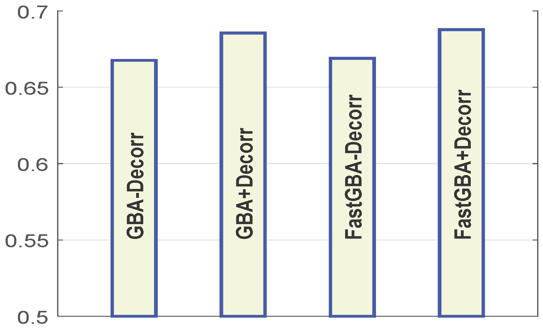
Using the shuffled metric (as shown in Figure 8), the results show that the GBA-Decorr and fast GBA-Decorr models give quite similar values when implemented without de-correlation, and a similar trend is exhibited by the GBA + Decorr and Fast GBA + Decorr models, which are implemented using de-correlated color space. For all algorithms, we used the following parameters: , , . Our results suggest that using de-correlation of the color image channels improves the performance of group-based saliency models. Furthermore, this implies that other saliency models can also benefit from using a de-correlated color space.
5. Future Work
We believe that our proposed approach on saliency can be extended to include three-dimensional image data (such as magnetic resonance imaging). In order to calculate saliency for three-dimensional data, we can use the symmetry groups for a cube.
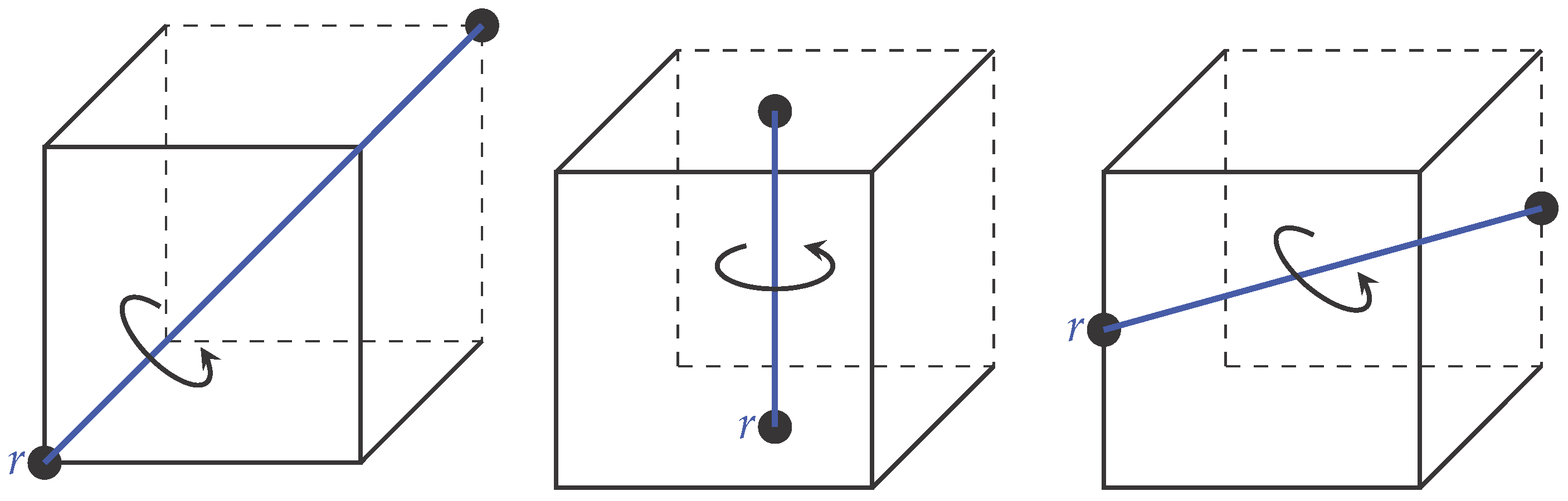
A cube has 48 symmetries that can be represented by the transformations of products of the groups and . is the symmetric group of degree two and has two elements: the identity and the permutation interchanging the two points [28]. is a symmetric group of degree four, i.e., all permutations on a set of size four [28]. This group has 24 elements that are obtained by rotations about opposite faces, opposite diagonals and opposite edges of the cube. For instance, Figure 9 shows the different rotational symmetries of the cube. We note that from the rotations along opposite diagonals, faces and edges, we get 8, 9 and 6 elements, respectively. These elements along with the identity form the 24 elements of the group.
Saliency for three-dimensional image data can be calculated by employing the same procedure as discussed in Section 3, but instead of computing in two-dimensional space using the group, we can calculate it in three-dimensional space using the transformations. For example, after dividing the three-dimensional scene into uniform sized cubes, we can rotate and reflect a cube and record the values associated with the transformations. The recorded values can be collected in a matrix and rescaled along each of the three planes, i.e., X-Y, Y-Z, Z-X, to get a three-dimensional feature map. The resulting feature maps corresponding to the 48 elements can be combined to get a representation of saliency for the three-dimensional scene. This is left as future work, and we hope that this will help future researchers to venture towards three-dimensional saliency.
6. Conclusions
In this article, first, we briefly describe the dihedral group that is used for calculating saliency in our proposed model. Second, our saliency model makes the two following changes in a latest state-of-the-art model known as group-based asymmetry: first, based on the properties of the dihedral group , we simplify the asymmetry calculations associated with the measurement of saliency. This results is an algorithm that reduces the number of calculations by at least half that makes it the fastest among the six best algorithms used in this research article. Two, in order to maximize the information across different chromatic and multi-resolution features, the color image space is de-correlated. We evaluate our algorithm against 10 state-of-the-art saliency models. Our results clearly show that by using optimal parameters for a given dataset our proposed model can outperform the best saliency algorithm in the literature. However, as the differences among the (few) best saliency models are small, we would like to suggest that our proposed model is among the best and the fastest among the best. In the end, as a part of future work, we suggest that our proposed approach on saliency can be extended to include three-dimensional image data.
Conflicts of Interest
The author declares no conflicts of interest.
References
- Suder, K.; Worgotter, F. The control of low-level information flow in the visual system. Rev. Neurosci. 2000, 11, 127–146. [Google Scholar] [CrossRef] [PubMed]
- Yang, J.; Yang, M.H. Top-down visual saliency via joint CRF and dictionary learning. In Proceedings of the 2012 IEEE Conference on Computer Vision and Pattern Recognition (CVPR), Providence, RI, USA, 16–21 June 2012; pp. 2296–2303.
- He, S.; Lau, R.W.; Yang, Q. Exemplar-Driven Top-Down Saliency Detection via Deep Association. In Proceedings of the IEEE Conference on Computer Vision and Pattern Recognition, Las Vegas, NV, USA, 27–30 June 2016.
- Koch, C.; Ullman, S. Shifts in selective visual attention: Towards the underlying neural circuitry. Hum. Neurobiol. 1985, 4, 219–227. [Google Scholar] [PubMed]
- Itti, L. Automatic Foveation for Video Compression Using a Neurobiological Model of Visual Attention. IEEE Trans. Image Process. 2004, 13, 1304–1318. [Google Scholar] [CrossRef] [PubMed]
- Yu, S.X.; Lisin, D.A. Image Compression based on Visual Saliency at Individual Scales. In Proceedings of the 5th International Symposium on Advances in Visual Computing Part I, Las Vegas, NV, USA, 30 November–2 December 2009; pp. 157–166.
- Alsam, A.; Rivertz, H.; Sharma, P. What the Eye Did Not See—A Fusion Approach to Image Coding. In Advances in Visual Computing; Bebis, G., Boyle, R., Parvin, B., Koracin, D., Fowlkes, C., Wang, S., Choi, M.H., Mantler, S., Schulze, J., Acevedo, D., et al., Eds.; Lecture Notes in Computer Science; Springer: Berlin, Germany; Heidelberg, Germany, 2012; Volume 7432, pp. 199–208. [Google Scholar]
- Alsam, A.; Rivertz, H.J.; Sharma, P. What the eye did not see–A fusion approach to image coding. Int. J. Artif. Intell. Tools 2013, 22, 1360014. [Google Scholar] [CrossRef]
- Siagian, C.; Itti, L. Biologically-Inspired Robotics Vision Monte-Carlo Localization in the Outdoor Environment. In Proceedings of the IEEE International Conference on Intelligent Robots and Systems, San Diego, CA, USA, 29 October–2 November 2007.
- Frintrop, S.; Jensfelt, P.; Christensen, H.I. Attentional Landmark Selection for Visual SLAM. In Proceedings of the IEEE/RSJ International Conference on Intelligent Robots and Systems, Beijing, China, 9–15 October 2006.
- Kadir, T.; Brady, M. Saliency, Scale and Image Description. Int. J. Comput. Vis. 2001, 45, 83–105. [Google Scholar] [CrossRef]
- Feng, X.; Liu, T.; Yang, D.; Wang, Y. Saliency based objective quality assessment of decoded video affected by packet losses. In Proceedings of the 15th IEEE International Conference on Image Processing, San Diego, CA, USA, 12–15 October 2008; pp. 2560–2563.
- Ma, Q.; Zhang, L. Saliency-Based Image Quality Assessment Criterion. In Advanced Intelligent Computing Theories and Applications. With Aspects of Theoretical and Methodological Issues; Huang, D.S., Wunsch, D.C.I., Levine, D., Jo, K.H., Eds.; Lecture Notes in Computer Science; Springer: Berlin, Germany; Heidelberg, Germany, 2008; Volume 5226, pp. 1124–1133. [Google Scholar]
- El-Nasr, M.; Vasilakos, A.; Rao, C.; Zupko, J. Dynamic Intelligent Lighting for Directing Visual Attention in Interactive 3-D Scenes. IEEE Trans. Comput. Intell. AI Games 2009, 1, 145–153. [Google Scholar] [CrossRef]
- Rosenholtz, R.; Dorai, A.; Freeman, R. Do predictions of visual perception aid design? ACM Trans. Appl. Percept. 2011, 8, 12:1–12:20. [Google Scholar] [CrossRef]
- Judd, T.; Ehinger, K.; Durand, F.; Torralba, A. Learning to predict where humans look. In Proceedings of the 2009 IEEE International Conference on Computer Vision (ICCV), Kyoto, Japan, 27 September–4 October 2009; pp. 2106–2113.
- Breazeal, C.; Scassellati, B. A Context-Dependent Attention System for a Social Robot. In Proceedings of the International Joint Conference on Artificial Intelligence (IJCAI), Stockholm, Sweden, 31 July–6 August 1999; pp. 1146–1153.
- Ajallooeian, M.; Borji, A.; Araabi, B.; Ahmadabadi, M.; Moradi, H. An application to interactive robotic marionette playing based on saliency maps. In Proceedings of the 18th IEEE International Symposium on Robot and Human Interactive Communication, Toyama, Japan, 27 September–2 October 2009; pp. 841–847.
- Itti, L.; Koch, C. A saliency-based search mechanism for overt and covert shifts of visual attention. Vis. Res. 2000, 40, 1489–1506. [Google Scholar] [CrossRef]
- Liu, T.; Sun, J.; Zheng, N.N.; Tang, X.; Shum, H.Y. Learning to Detect A Salient Object. In Proceedings of the 2007 IEEE Conference on Computer Vision and Pattern Recognition, Minneapolis, MN, USA, 18–23 June 2007.
- Achanta, R.; Estrada, F.; Wils, P.; Süsstrunk, S. Salient region detection and segmentation. In Proceedings of the 6th International Conference on Computer Vision Systems, Santorini, Greece, 12–15 May 2008; pp. 66–75.
- Erdem, E.; Erdem, A. Visual saliency estimation by nonlinearly integrating features using region covariances. J. Vis. 2013, 13, 1–20. [Google Scholar] [CrossRef] [PubMed]
- He, S.; Lau, R.W.H.; Liu, W.; Huang, Z.; Yang, Q. SuperCNN: A Superpixelwise Convolutional Neural Network for Salient Object Detection. Int. J. Comput. Vis. 2015, 115, 330–344. [Google Scholar] [CrossRef]
- Alsam, A.; Sharma, P.; Wrålsen, A. Asymmetry as a Measure of Visual Saliency. Lecture Notes in Computer Science (LNCS); Springer-Verlag Berlin Heidelberg: Berlin, Germany; Heidelberg, Germany, 2013; Volume 7944, pp. 591–600. [Google Scholar]
- Alsam, A.; Sharma, P.; Wrålsen, A. Calculating saliency using the dihedral group D4. J. Imaging Sci. Technol. 2014, 58, 10504:1–10504:12. [Google Scholar] [CrossRef]
- Itti, L.; Koch, C.; Niebur, E. A Model of Saliency-Based Visual Attention for Rapid Scene Analysis. IEEE Trans. Pattern Anal. Mach. Intell. 1998, 20, 1254–1259. [Google Scholar] [CrossRef]
- Garcia-Diaz, A.; Fdez-Vidal, X.R.; Pardo, X.M.; Dosil, R. Saliency from hierarchical adaptation through decorrelation and variance normalization. Image Vis. Comput. 2012, 30, 51–64. [Google Scholar] [CrossRef]
- Dummit, D.S.; Foote, R.M. Abstract Algebra, 3rd ed.; John Wiley & Sons: Hoboken, NJ, USA, 2004. [Google Scholar]
- Lenz, R. Using representations of the dihedral groups in the design of early vision filters. In Proceedings of the IEEE International Conference on Acoustics, Speech, and Signal Processing (ICASSP-93), Minneapolis, MN, USA, 27–30 April 1993; pp. 165–168.
- Lenz, R. Investigation of Receptive Fields Using Representations of the Dihedral Groups. J. Vis. Commun. Image Represent. 1995, 6, 209–227. [Google Scholar] [CrossRef]
- Foote, R.; Mirchandani, G.; Rockmore, D.N.; Healy, D.; Olson, T. A wreath product group approach to signal and image processing. I. Multiresolution analysis. IEEE Trans. Signal Process. 2000, 48, 102–132. [Google Scholar] [CrossRef]
- Chang, W.Y. Image Processing with Wreath Products. Master’s Thesis, Harvey Mudd College, Claremont, CA, USA, 2004. [Google Scholar]
- Lenz, R.; Bui, T.H.; Takase, K. A group theoretical toolbox for color image operators. In Proceedings of the IEEE International Conference on Image Processing, Genoa, Italy, 11–14 September 2005; Volume 3, pp. 557–560.
- Sharma, P. Evaluating visual saliency algorithms: Past, present and future. J. Imaging Sci. Technol. 2015, 59, 50501:1–50501:17. [Google Scholar] [CrossRef] [Green Version]
- Tatler, B.W.; Baddeley, R.J.; Gilchrist, I.D. Visual correlates of fixation selection: Effects of scale and time. Vis. Res. 2005, 45, 643–659. [Google Scholar] [CrossRef] [PubMed]
- Tatler, B.W. The central fixation bias in scene viewing: Selecting an optimal viewing position independently of motor biases and image feature distributions. J. Vis. 2007, 7, 1–17. [Google Scholar] [CrossRef] [PubMed]
- Tseng, P.H.; Carmi, R.; Cameron, I.G.M.; Munoz, D.P.; Itti, L. Quantifying center bias of observers in free viewing of dynamic natural scenes. J. Vis. 2009, 9, 1–16. [Google Scholar] [CrossRef] [PubMed]
- Zhang, L.; Tong, M.H.; Marks, T.K.; Shan, H.; Cottrell, G.W. SUN: A Bayesian framework for saliency using natural statistics. J. Vis. 2008, 8, 1–20. [Google Scholar] [CrossRef] [PubMed]
- Fawcett, T. ROC Graphs with Instance-Varying Costs. Pattern Recognit. Lett. 2004, 27, 882–891. [Google Scholar] [CrossRef]
- Bruce, N.D.B.; Tsotsos, J.K. Saliency Based on Information Maximization. In Proceedings of the Neural Information Processing Systems conference (NIPS 2005), Vancouver, BC, Canada, 5–10 December 2005; pp. 155–162.
- Hou, X.; Zhang, L. Saliency Detection: A Spectral Residual Approach. In Proceedings of the 2007 IEEE Conference on Computer Vision and Pattern Recognition, Minneapolis, MN, USA, 17–22 June 2007; pp. 1–8.
- Schauerte, B.; Stiefelhagen, R. Predicting Human Gaze using Quaternion DCT Image Signature Saliency and Face Detection. In Proceedings of the IEEE Workshop on the Applications of Computer Vision (WACV), Breckenridge, CO, USA, 9–11 January 2012.
- Harel, J.; Koch, C.; Perona, P. Graph-Based Visual Saliency. In Proceedings of Neural Information Processing Systems (NIPS); MIT Press: Cambridge, MA, USA, 2006; pp. 545–552. [Google Scholar]
- Borji, A.; Itti, L. Exploiting Local and Global Patch Rarities for Saliency Detection. In Proceedings of the IEEE Conference on Computer Vision and Pattern Recognition (CVPR), Providence, RI, USA, 18–20 June 2012; pp. 1–8.
- Borji, A.; Sihite, D.N.; Itti, L. Quantitative Analysis of Human-Model Agreement in Visual Saliency Modeling: A Comparative Study. IEEE Trans. Image Process. 2013, 22, 55–69. [Google Scholar] [CrossRef] [PubMed]
Figure 1.
Polygons for n = 3, 4, 5 and 6 and the associated reflection symmetries. Here, we can see that when n is odd, each axis of symmetry connects the vertex with the midpoint of the opposite side. When n is even, there are n/2 symmetry axes connecting the midpoints of opposite sides and n/2 symmetry axes connecting opposite vertices.
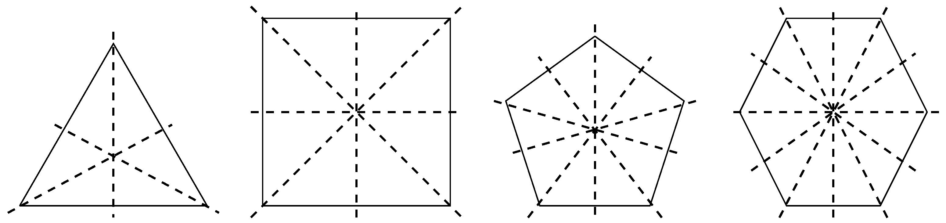
Figure 2.
Rotation of the square by 90counterclockwise.

Figure 3.
Original group-based algorithm proposed by Alsam et al. [24,25], the figure shows an example image (from [16]) along with the associated saliency map. The figure on the top-right shows the eight group transformations pertaining to a square block of an image. Bottom-right figures show the asymmetry calculations for square blocks pertaining to uniform and non-uniform regions. We can see that for uniform regions, this value is close to zero. Please note that bright locations represent higher values, and dark locations represent low values.

Figure 4.
Figure shows a test image (from the database [16]) and the associated saliency maps from different saliency algorithms used in the paper.
Figure 4.
Figure shows a test image (from the database [16]) and the associated saliency maps from different saliency algorithms used in the paper.


Figure 5.
Ranking of different saliency models using the shuffled metric. The results are obtained from the fixation data of 463 landscape images and fifteen observers.
Figure 5.
Ranking of different saliency models using the shuffled metric. The results are obtained from the fixation data of 463 landscape images and fifteen observers.

Figure 6.
Average run time across 463 landscape images for different saliency models: Itti = 0.60, Hou = 0.05, Spec = 0.07, GBA = 20.13, AIM = 31.75, LG = 15.70, Erdem = 23.35, Fast GBA = 0.65, AWS = 10.27. All run times are in seconds. For a better visualization, we use the natural logarithm of the average run times.
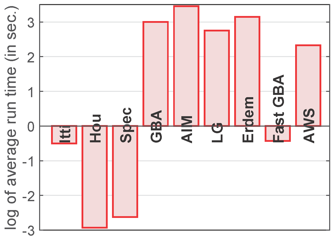
Figure 7.
The results obtained by using the shuffled metric for the three variables are shown in the first row. The figure on the top-left shows the shuffled values for , with the red, green and blue lines depicting as 1, 2 and 3 respectively, while, the figure on the top-right shows the shuffled values for . In the second row, we show the average run time of the algorithm for the different values of , b and .
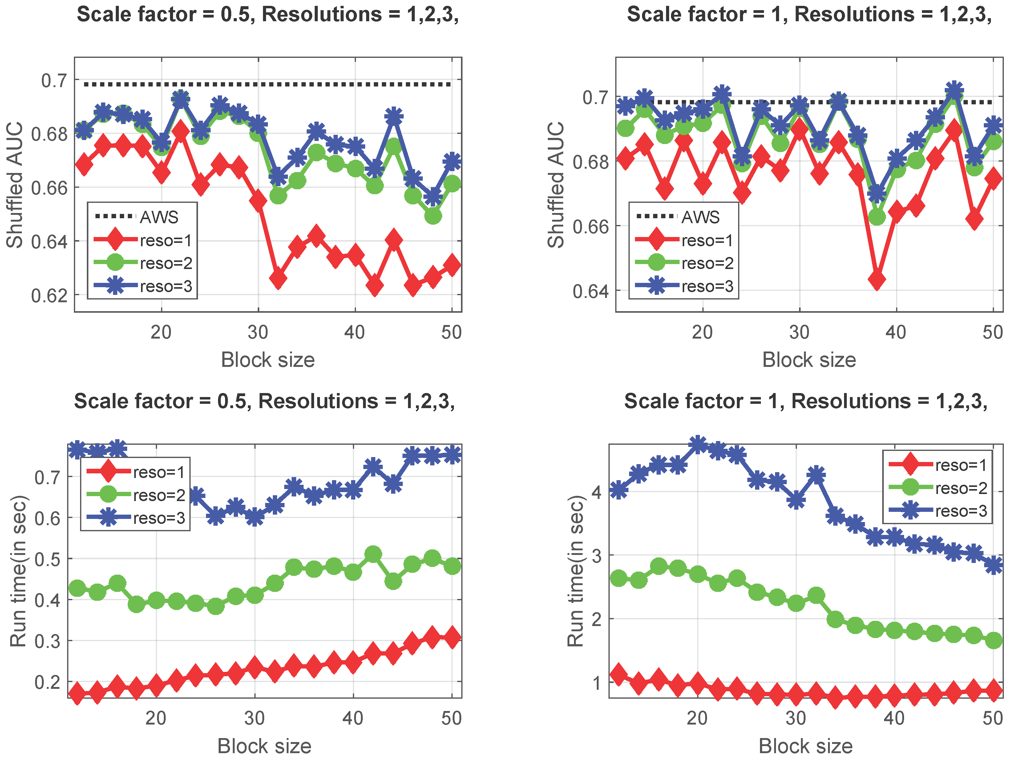
Figure 8.
GBA-Decorr and fast GBA-Decorr models give quite similar values when implemented without de-correlation, and a similar trend is exhibited by the GBA + Decorr and fast GBA + Decorr models, which are implemented using de-correlated color space. For all algorithms, we used the following parameters , , . The results are obtained from the fixation data of 463 landscape images and fifteen observers using the shuffled metric.

Figure 9.
(Left) Number of axes with opposite diagonals like this = 4. We can rotate by 120 or 240 degrees around these axes. These operations give eight elements. (Center) Number of axes with opposite faces like this = 3. We can either rotate by 90, 180 or 270 degrees around these axes. These operations give nine elements. (Right) Number of axes with opposite edges like this = 6. We can rotate by 180 degrees around these axes. These operations give six elements.

© 2016 by the author; licensee MDPI, Basel, Switzerland. This article is an open access article distributed under the terms and conditions of the Creative Commons Attribution (CC-BY) license (http://creativecommons.org/licenses/by/4.0/).
Share and Cite
MDPI and ACS Style
Sharma, P. Modeling Bottom-Up Visual Attention Using Dihedral Group D4. Symmetry 2016, 8, 79. https://doi.org/10.3390/sym8080079
AMA Style
Sharma P. Modeling Bottom-Up Visual Attention Using Dihedral Group D4. Symmetry. 2016; 8(8):79. https://doi.org/10.3390/sym8080079
Chicago/Turabian StyleSharma, Puneet. 2016. "Modeling Bottom-Up Visual Attention Using Dihedral Group D4" Symmetry 8, no. 8: 79. https://doi.org/10.3390/sym8080079
Note that from the first issue of 2016, this journal uses article numbers instead of page numbers. See further details here.