
A Data Mining Approach for Cardiovascular Disease Diagnosis Using Heart Rate Variability and Images of Carotid Arteries


Abstract
:1. Introduction
- (1)
- Extracting diagnostic feature vectors: the feature vectors significant to disease diagnosis are extracted by applying image processing to the CA images taken by ultrasound;
- (2)
- Evaluation on feature vector and classification method for diagnosis of CVD: some diagnostic feature vectors that are significant by types of CVD through statistical analysis of the data should be selected as a preprocessing step. Classification or prediction algorithm is applied to the selected diagnostic feature vectors for CVD, and the vectors were evaluated.
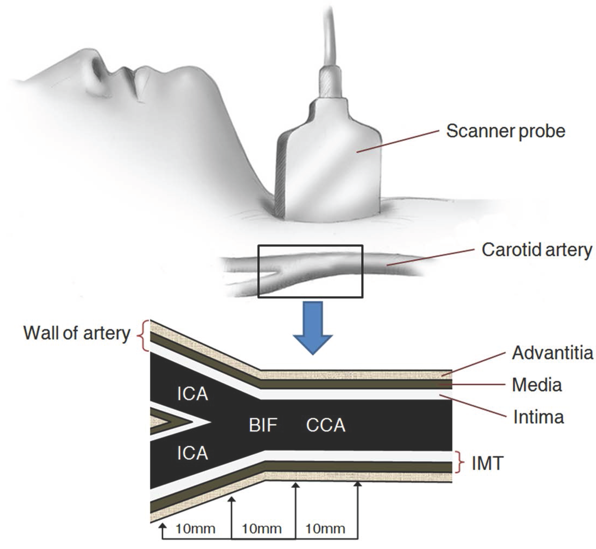
2. Carotid Artery Scanning and Image Processing
- (1)
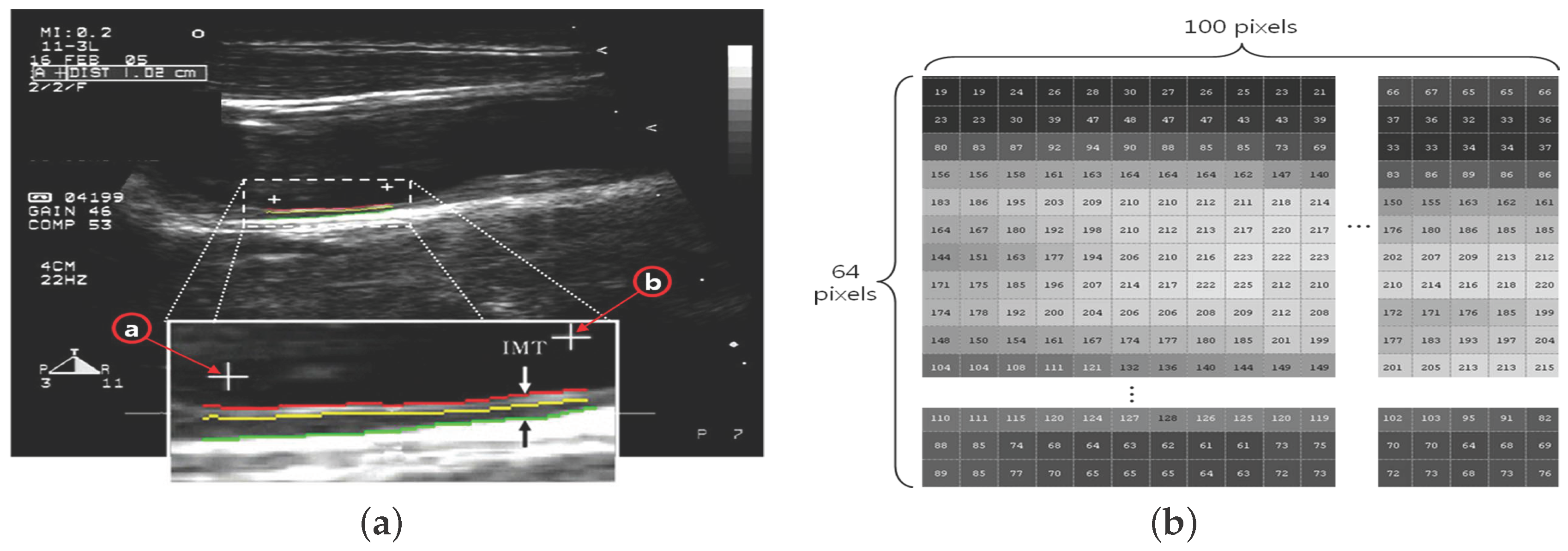
- The ROI image with pixels is acquired by defining the area of two ’+’ markers (from to ) on the image of the carotid IMT in Figure 2a;
- (2)
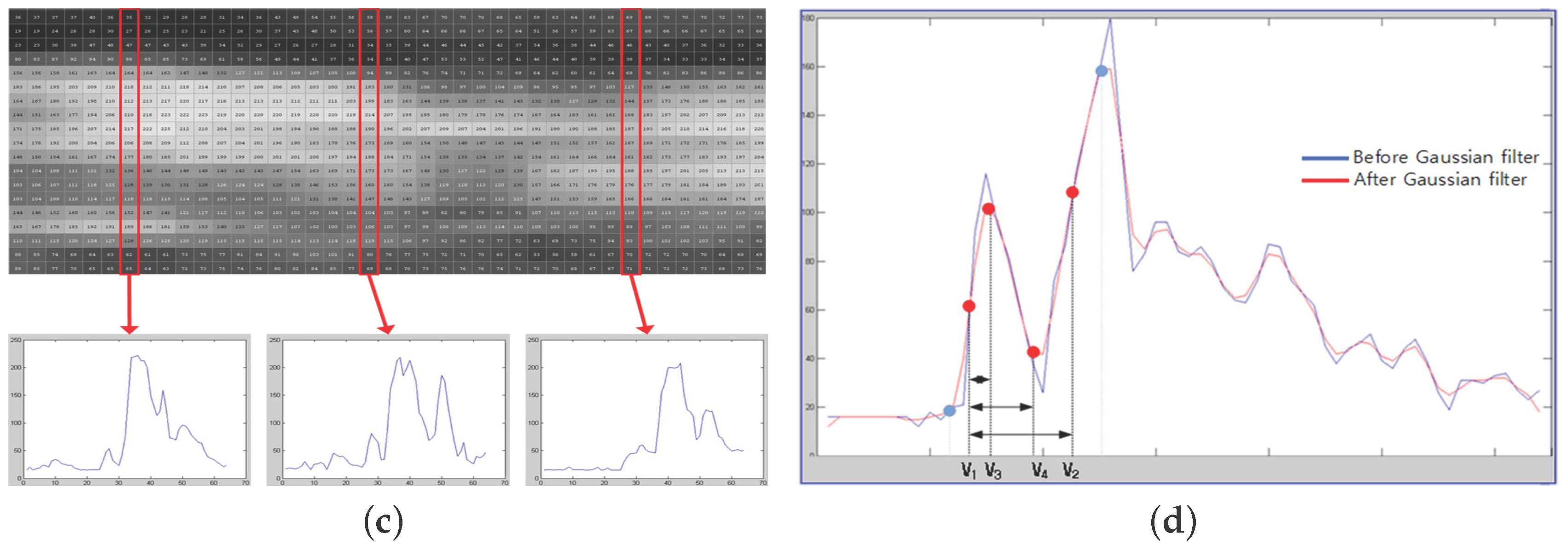
- Each pixel is expressed by a number in the range of 0– for the brightness (Figure 2b);
- (3)
- The trend of variation is shown in a graph in a vertical line (Figure 2c);
- (4)
- Thirty vertical lines are randomly selected as samples among a total of 100 vertical lines (Figure 2d);
- (5)
- The difference between and is calculated using the 30 random samples of vertical lines;
- (6)
- Only IMT values within one sigma in Gaussian distribution are extracted;
- (7)
- Four basic feature vectors are extracted and an average value is calculated;
- (8)
- The other 18 additional feature vectors are extracted through a calculation using the four basic feature vectors in Figure 2d, and the mean value is obtained.
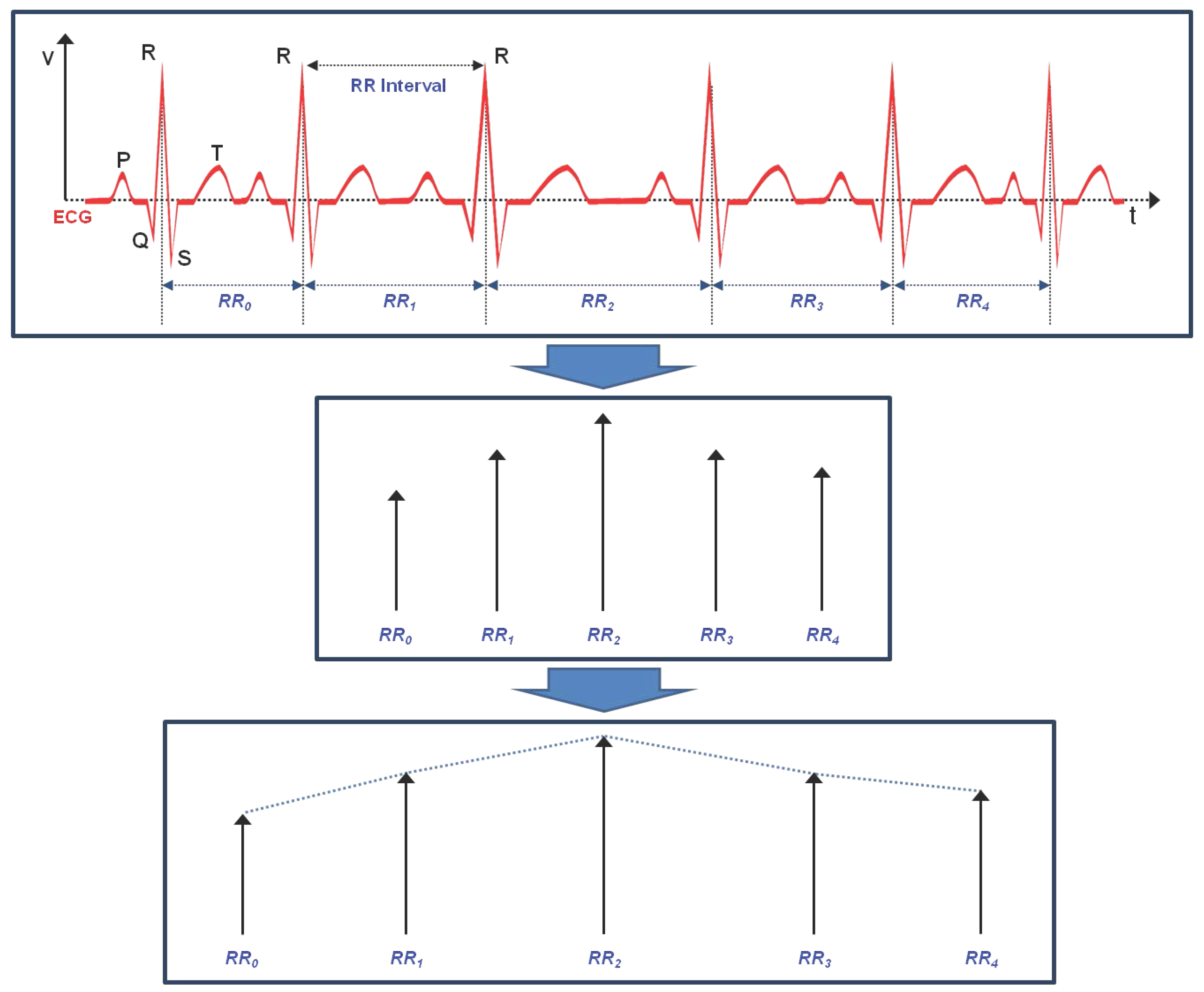
3. Linear and Non-Linear Feature Vectors of HRV
3.1. Linear Feature Vectors in Time Domain
3.2. Linear Feature Vectors in Frequency Domain
- (1)
- Total power (), from 0 Hz to 0.4 Hz;
- (2)
- Very Low Frequency () power, from 0 Hz to 0.04 Hz;
- (3)
- Low Frequency () power, from 0.04 Hz to 0.15 Hz;
- (4)
- High Frequency () power, from 0.15 Hz to 0.4 Hz;
- (5)
- Normalized value of ();
- (6)
- Normalized value of ();
- (7)
- The ratio of and ().
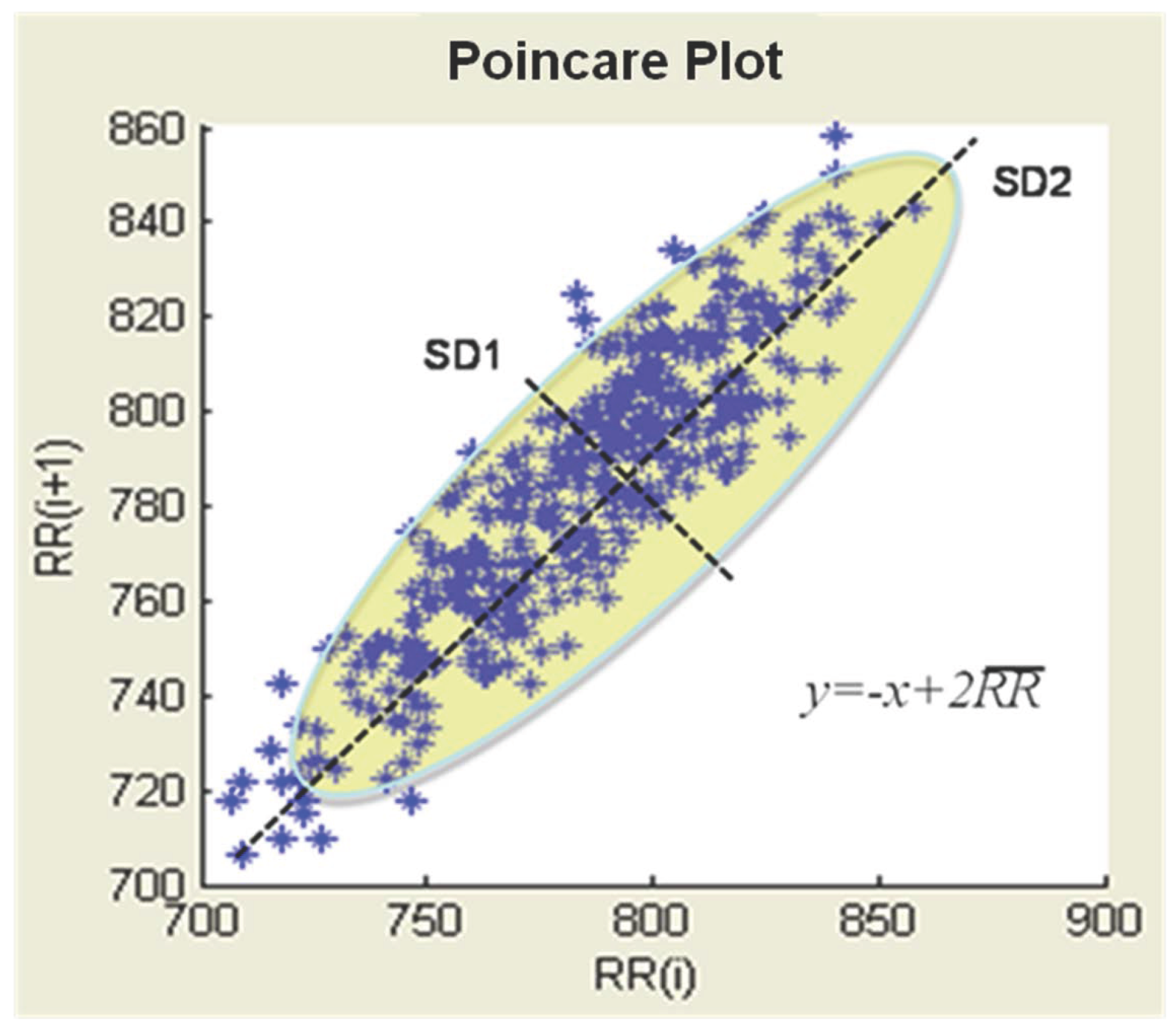
3.3. Poincare Plot of Nonlinear Feature Vectors
3.4. A Non-Linear Vector: Approximate Entropy (ApEn)
3.5. Hurst Exponent (H) Non-Linear Vector)
3.6. Exponent α of the Spectrum () Non-Linear Vector
4. Evaluation of Diagnostic Feature Vectors
4.1. Data Preprocessing
4.2. Verification of Feature Vectors Using Classification Methods
4.2.1. Neural Networks
4.2.2. Bayesian Network
4.2.3. Decision Tree Induction (C4.5)
4.2.4. Support Vector Machine (SVM)
4.2.5. Classification Based on Multiple Association Rules (CMAR)
- weka.classifiers.bayes.BayesNet (TAN)
- weka.classifiers.tree.j48.J48 (C4.5)
- weka.classifiers.funtions.SMO (SVM)
- weka.classifiers.functions.MultilayerPerceptron (MLP)
5. Conclusions
Acknowledgments
Author Contributions
Conflicts of Interest
References
- WHO. The Top 10 Causes of Death. WHO Report. Available online: http://www.who.int/mediacentre/factsheets/fs310/en/ (accessed on 1 April 2015).
- Korea National Statistical Office. Statistics Report of Causes of Death. Available online: http://kosis.kr/statHtml/statHtml.do?orgId=101&tblId=DT_1B34E02&conn_path=I2 (accessed on 1 April 2015).
- Ryu, K.S.; Park, H.W.; Park, S.H.; Shon, H.S.; Ryu, K.H.; Lee, D.G.; Bashir, M.E.; Lee, J.H.; Kim, S.M.; Lee, S.Y.; et al. Comparison of clinical outcomes between culprit vessel only and multivessel percutaneous coronary intervention for ST-segment elevation myocardial infarction patients with multivessel coronary diseases. J. Geriatr. Cardiol. 2015, 12, 208. [Google Scholar] [PubMed]
- Lee, D.G.; Ryu, K.S.; Bashir, M.; Bae, J.W.; Ryu, K.H. Discovering medical knowledge using association rule mining in young adults with acute myocardial infarction. J. Med. Syst. 2013, 37, 1–10. [Google Scholar] [CrossRef] [PubMed]
- Bae, J.H.; Seung, K.B.; Jung, H.O.; Kim, K.Y.; Yoo, K.D.; Kim, C.M.; Cho, S.W.; Cho, S.K.; Kim, Y.K.; Rhee, M.Y.; et al. Analysis of Korean carotid intima-media thickness in Korean healthy subjects and patients with risk factors: Korea multi-center epidemiological study. Korean Circ. J. 2005, 35, 513–524. [Google Scholar] [CrossRef]
- Cheng, K.S.; Mikhailidis, D.P.; Hamilton, G.; Seifalian, A.M. A review of the carotid and femoral intima-media thickness as an indicator of the presence of peripheral vascular disease and cardiovascular risk factors. Cardiovasc. Res. 2002, 54, 528–538. [Google Scholar] [CrossRef]
- Nambi, V.; Chambless, L.; He, M.; Folsom, A.R.; Mosley, T.; Boerwinkle, E.; Ballantyne, C.M. Common carotid artery intima–media thickness is as good as carotid intima–media thickness of all carotid artery segments in improving prediction of coronary heart disease risk in the Atherosclerosis Risk in Communities (ARIC) study. Eur. Heart J. 2012, 33, 183–190. [Google Scholar] [CrossRef] [PubMed]
- Tarvainen, M.P.; Niskanen, J.P.; Lipponen, J.A.; Ranta-Aho, P.O.; Karjalainen, P.A. Kubios HRV—Heart Rate Variability Analysis Software. Comp. Method. Progr. Biomed. 2014, 113, 210–220. [Google Scholar] [CrossRef] [PubMed]
- dos Santos, L.; Barroso, J.J.; Macau, E.E.; de Godoy, M.F. Application of an automatic adaptive filter for heart rate variability analysis. Med. Eng. Phys. 2013, 35, 1778–1785. [Google Scholar] [CrossRef] [PubMed]
- ChuDuc, H.; NguyenPhan, K.; NguyenViet, D. A review of heart rate variability and its applications. APCBEE Proced. 2013, 7, 80–85. [Google Scholar] [CrossRef]
- Pumprla, J.; Howorka, K.; Groves, D.; Chester, M.; Nolan, J. Functional assessment of heart rate variability: Physiological basis and practical applications. Int. J. Cardiol. 2002, 84, 1–14. [Google Scholar] [CrossRef]
- Bae, J.H.; Kim, W.S.; Rihal, C.S.; Lerman, A. Individual Measurement and Significance of Carotid Intima, Media, and Intima–Media Thickness by B-Mode Ultrasonographic Image Processing. Arterioscler. Thromb. Vasc. Biol. 2006, 26, 2380–2385. [Google Scholar] [CrossRef] [PubMed]
- Piao, M.; Lee, H.G.; Pok, C.; Ryu, K.H. A data mining approach for dyslipidemia disease prediction using carotid arterial feature vectors. In Proceedings of the 2010 2nd International Conference on Computer Engineering and Technology (ICCET), Chengdu, China, 16–18 April 2010; Volume 2, pp. 171–175.
- Tompkins, W.J. Biomedical Digital Signal Processing: C Language Examples and Laboratory Experiments for the IBM PC; Prentice Hall, Inc.: Upper Saddle River, NJ, USA, 1993. [Google Scholar]
- Lee, H.G.; Kim, W.S.; Noh, K.Y.; Shin, J.H.; Yun, U.; Ryu, K.H. Coronary artery disease prediction method using linear and nonlinear feature of heart rate variability in three recumbent postures. Inf. Syst. Front. 2009, 11, 419–431. [Google Scholar] [CrossRef]
- Brennan, M.; Palaniswami, M.; Kamen, P. Do existing measures of Poincare plot geometry reflect nonlinear features of heart rate variability? IEEE Trans. Biomed. Eng. 2001, 48, 1342–1347. [Google Scholar] [CrossRef] [PubMed]
- Takens, F. Detecting strange attractors in turbulence. In Dynamical Systems and Turbulence, Warwick 1980; Lecture Notes in Mathematics; Springer Verlag: Berlin, Germany, 1981; Volume 898, pp. 366–381. [Google Scholar]
- Bhanot, G.; Alexe, G.; Venkataraghavan, B.; Levine, A.J. A robust meta-classification strategy for cancer detection from MS data. Proteomics 2006, 6, 592–604. [Google Scholar] [CrossRef] [PubMed]
- Witten, I.H.; Frank, E. Data Mining: Practical Machine Learning Tools and Techniques, 2nd ed.; Morgan Kaufmann Publishers: San Francisco, CA, USA, 2005. [Google Scholar]
- Cheng, J.; Greiner, R. Comparing Bayesian network classifiers. In Proceedings of the Fifteenth Conference on Uncertainty in Artificial Intelligence, Stockholm, Sweden, 30 July–1 August 1999; pp. 101–108.
- Quinlan, J.R. C4.5: Programs for Machine Learning; Morgan Kaufmann Publishers: San Mateo, CA, USA, 1993. [Google Scholar]
- Li, W.; Han, J.; Pei, J. CMAR: Accurate and efficient classification based on multiple class-association rules. In Proceedings of the IEEE International Conference on Data Mining 2001 (ICDM 2001), San Jose, CA, USA, 29 November–2 December 2001; pp. 369–376.
- Han, J.; Pei, J.; Yin, Y.; Mao, R. Mining frequent patterns without candidate generation: A frequent-pattern tree approach. Data Min. Knowl. Discov. 2004, 8, 53–87. [Google Scholar] [CrossRef]
- Lairenjam, B.; Wasan, S.K. Neural network with classification based on multiple association rule for classifying mammographic data. In Intelligent Data Engineering and Automated Learning-IDEAL 2009; Springer Berlin Heidelberg: Berlin, Heidelberg, Germany, 2009; pp. 465–476. [Google Scholar]
- Coenen, F. The LUCS-KDD Software Library. 2004. Available online: http://cgi.csc.liv.ac.uk/%7efrans/KDD/Software/ (accessed on 6 June 2016).
- Piao, Y.; Piao, M.; Jin, C.H.; Shon, H.S.; Chung, J.M.; Hwang, B.; Ryu, K.H. A New Ensemble Method with Feature Space Partitioning for High-Dimensional Data Classification. Math. Probl. Eng. 2015. [Google Scholar] [CrossRef]
- Lee, H.G.; Choi, Y.H.; Jung, H.; Shin, Y.H. Subspace Projection–Based Clustering and Temporal ACRs Mining on MapReduce for Direct Marketing Service. ETRI J. 2015, 37, 317–327. [Google Scholar] [CrossRef]


| Feature vector | Index | Description |
|---|---|---|
| Carotid basic feature | Starting point of intima | |
| Starting point of adventitia | ||
| Max. point between and | ||
| Min. point between and | ||
| Carotid calculated feature | Distance between and | |
| Area of the vector | ||
| Value of the point | ||
| Distance between and | ||
| Area of the vector | ||
| Value of the point | ||
| Distance between and | ||
| Area of the vector | ||
| Slope between and | ||
| Slope between and | ||
| Slope between and | ||
| - | ||
| - | ||
| Standard deviation between and | ||
| Variance between and | ||
| Skewness between and | ||
| Kurtosis between and | ||
| Moment between and | ||
| IMT | Intima-media thickness |
| Feature Vector | Description | ||
|---|---|---|---|
| Normalized low frequency power (). | |||
| Normalized high frequency power (). | |||
| The ratio of low- and high-frequency power. | |||
| The mean of RR intervals. | |||
| SDRR | Standard deviation of the RR intervals. | ||
| SDSD | Standard deviation of the successive differences RR intervals. | ||
| Standard deviation of the distance of from the line in the Poincare | |||
| Standard deviation of the distance of from the line in the Poincare | |||
| The ratio to | |||
| Approximate Entropy | |||
| H | Hurst Exponent | ||
| 1/f scaling of Fourier spectra | |||
| Group | N | Sex (Male/Female) | Age (Years) |
|---|---|---|---|
| AP | 102 | 50/52 | 59.98±8.41 |
| Control | 72 | 40/46 | 56.70±9.23 |
| ACS | 40 | 18/22 | 58.94±8.68 |
| Rank | CA | HRV | CA+HRV | |||
|---|---|---|---|---|---|---|
| Feature | RS() | Feature | RS() | Feature | RS() | |
| 1 | 1.000 | 0.999 | 1.000 | |||
| 2 | 1.000 | 0.998 | 1.000 | |||
| 3 | 0.998 | 0.993 | 0.998 | |||
| 4 | 0.997 | 0.991 | 0.997 | |||
| 5 | 0.997 | 0.986 | 0.986 | |||
| 6 | 0.995 | H | 0.984 | 0.985 | ||
| 7 | 0.989 | 0.975 | 0.979 | |||
| 8 | 0.989 | 0.968 | 0.979 | |||
| 9 | 0.975 | 0.967 | 0.965 | |||
| 10 | 0.968 | 0.961 | 0.965 | |||
| 11 | 0.968 | 0.958 | H | 0.965 | ||
| 12 | 0.967 | 0.955 | 0.963 | |||
| 13 | 0.966 | 0.962 | ||||
| 14 | 0.962 | 0.962 | ||||
| 15 | 0.961 | 0.960 | ||||
| 16 | 0.953 | 0.958 | ||||
| 17 | 0.955 | |||||
| 18 | 0.954 | |||||
| 19 | 0.952 | |||||
| 20 | 0.951 | |||||
| Classifier | CA | HRV | CA+HRV | Class | ||||||
|---|---|---|---|---|---|---|---|---|---|---|
| (Using 16 Features) | (Using 12 Features) | (Using 20 Features) | ||||||||
| Precision | Recall | Precision | Recall | Precision | Recall | |||||
| 0.701 | 0.754 | 0.727 | 0.681 | 0.749 | 0.713 | 0.763 | 0.913 | 0.831 | AP | |
| 0.707 | 0.714 | 0.711 | 0.696 | 0.713 | 0.704 | 0.835 | 0.749 | 0.790 | Control | |
| 0.519 | 0.409 | 0.457 | 0.480 | 0.336 | 0.395 | 0.833 | 0.568 | 0.675 | ACS | |
| 0.627 | 0.782 | 0.696 | 0.589 | 0.749 | 0.659 | 0.660 | 0.871 | 0.751 | AP | |
| 0.669 | 0.541 | 0.598 | 0.632 | 0.532 | 0.578 | 0.768 | 0.553 | 0.643 | Control | |
| 0.595 | 0.425 | 0.496 | 0.501 | 0.297 | 0.373 | 0.725 | 0.499 | 0.591 | ACS | |
| C4.5 | 0.656 | 0.716 | 0.685 | 0.669 | 0.727 | 0.697 | 0.734 | 0.870 | 0.796 | AP |
| 0.722 | 0.706 | 0.714 | 0.727 | 0.711 | 0.719 | 0.846 | 0.742 | 0.790 | Control | |
| 0.488 | 0.394 | 0.436 | 0.463 | 0.378 | 0.416 | 0.645 | 0.482 | 0.552 | ACS | |
| SVM | 0.756 | 0.810 | 0.782 | 0.685 | 0.804 | 0.740 | 0.872 | 0.854 | 0.863 | AP |
| 0.795 | 0.735 | 0.764 | 0.803 | 0.745 | 0.773 | 0.864 | 0.926 | 0.894 | Control | |
| 0.621 | 0.592 | 0.606 | 0.376 | 0.258 | 0.305 | 0.718 | 0.664 | 0.690 | ACS | |
| CMAR | 0.719 | 0.814 | 0.764 | 0.617 | 0.818 | 0.703 | 0.839 | 0.945 | 0.889 | AP |
| 0.669 | 0.769 | 0.716 | 0.702 | 0.774 | 0.736 | 0.836 | 0.845 | 0.840 | Control | |
| 0.694 | 0.462 | 0.554 | 0.542 | 0.235 | 0.328 | 0.855 | 0.692 | 0.765 | ACS | |
| Classifier | CA (Using 16 Features) | HRV (Using 12 Features) | CA+HRV (Using 20 Features) |
|---|---|---|---|
| NNs (MLP) | 0.405 | 0.442 | 0.293 |
| BayesNet (TAN) | 0.443 | 0.509 | 0.395 |
| C4.5 | 0.422 | 0.426 | 0.342 |
| SVM | 0.301 | 0.437 | 0.216 |
| CMAR | 0.355 | 0.472 | 0.201 |
| Features | Classifier | Actual Class | Predicted Class | ||
|---|---|---|---|---|---|
| AP (%) | Control (%) | ACS (%) | |||
| SVM | AP | 81.01 | 6.29 | 12.7 | |
| Control | 24.4 | 73.51 | 2.09 | ||
| ACS | 22.66 | 18.12 | 59.22 | ||
| CMAR | AP | 81.37 | 7.84 | 10.79 | |
| Control | 18.04 | 76.89 | 5.07 | ||
| ACS | 26.92 | 26.92 | 46.16 | ||
| SVM | AP | 80.4 | 6.05 | 13.55 | |
| Control | 20.85 | 74.52 | 4.63 | ||
| ACS | 56.66 | 17.5 | 25.84 | ||
| CMAR | AP | 81.82 | 7.28 | 10.9 | |
| Control | 18.13 | 77.43 | 4.44 | ||
| ACS | 53.94 | 22.57 | 23.49 | ||
| SVM | AP | 85.42 | 4.6 | 9.98 | |
| Control | 7.1 | 92.55 | 0.35 | ||
| ACS | 19.06 | 14.55 | 66.39 | ||
| CMAR | AP | 94.51 | 1.57 | 3.92 | |
| Control | 9.27 | 84.51 | 6.22 | ||
| ACS | 16.39 | 14.38 | 69.23 | ||
© 2016 by the authors; licensee MDPI, Basel, Switzerland. This article is an open access article distributed under the terms and conditions of the Creative Commons Attribution (CC-BY) license (http://creativecommons.org/licenses/by/4.0/).
Share and Cite
Kim, H.; Ishag, M.I.M.; Piao, M.; Kwon, T.; Ryu, K.H. A Data Mining Approach for Cardiovascular Disease Diagnosis Using Heart Rate Variability and Images of Carotid Arteries. Symmetry 2016, 8, 47. https://doi.org/10.3390/sym8060047
Kim H, Ishag MIM, Piao M, Kwon T, Ryu KH. A Data Mining Approach for Cardiovascular Disease Diagnosis Using Heart Rate Variability and Images of Carotid Arteries. Symmetry. 2016; 8(6):47. https://doi.org/10.3390/sym8060047
Chicago/Turabian StyleKim, Hyeongsoo, Musa Ibrahim M. Ishag, Minghao Piao, Taeil Kwon, and Keun Ho Ryu. 2016. "A Data Mining Approach for Cardiovascular Disease Diagnosis Using Heart Rate Variability and Images of Carotid Arteries" Symmetry 8, no. 6: 47. https://doi.org/10.3390/sym8060047