Loss of Temporal Homogeneity and Symmetry in Statistical Systems: Deterministic Versus Stochastic Dynamics

Abstract

A detailed analysis of deterministic (one-to-one) and stochastic (one-to-many) dynamics establishes that $dS/dt$ > 0 is only consistent with the latter, which contains violation of temporal symmetry and homogeneity. We observe that the former only supports $dS/dt$ = 0 and cannot give rise to Boltzmann’s molecular chaos assumption. The ensemble average is more meaningful than the temporal average, especially in non-equilibrium statistical mechanics of systems confined to disjoint phase space components, which commonly occurs at low temperatures. We propose that the stochasticity arises from extra degrees of freedom, which are not part of the system. We provide a simple resolution of the recurrence and irreversibility paradoxes.

1. Introduction

One of the most important developments in theoretical physics is the use of symmetry in studying physical phenomena. The symmetry properties of a physical system determine how it evolves in time; see for example, Noether’s theorem applicable to systems modeled by a Hamiltonian [1]. Apart from continuous symmetries (global or local), there are also discrete symmetries such as reflection, time-reversal invariance, etc. that are also found useful in Nature [2]. Among all these symmetries, we will only be concerned with the two symmetries involving time in this review, which are the following:

• Temporal symmetry due to time-reversal invariance. The time reversal

  $$t\to t^{\prime }\equiv -t$$

  (1)

  corresponds to a discrete transformation of time t and the invariance under this transformation ensures that forward and backward evolution in time are physically indistinguishable.
• Temporal Homogeneity due to shift in the origin of time. The shift

  $$t\to t^{\prime }\equiv t+t_0$$

  (2)

  by a constant $t_0$ for all times t corresponds to a continuous transformation when $t_0$ becomes infinitesimal, and the invariance under the shift ensures that the energy remains a constant in the evolution of the system.

Consider a projectile in the $x-y$ plane, which leaves the ground from the origin ${\mathbf{r}}_0\equiv (0,0)$ at time $t=-\tau$ with a velocity ${\mathbf{v}}_0\equiv (v_{0x},v_{0y})$ [3]. It reaches the ground again at ${\mathbf{r}}_1\equiv (R,0)$ at time $t=0$ with a velocity ${\mathbf{v}}_1\equiv (v_{0x},-v_{0y})$. The initial state of the projectile is $({\mathbf{r}}_0,{\mathbf{v}}_0)$ and its final state is $({\mathbf{r}}_1,{\mathbf{v}}_1)$. For time-reversed states, the initial and final states are interchanged with reversed velocities:

$$\begin{array}{cc}\hfill ({\mathbf{r}}_0,{\mathbf{v}}_0)& \iff ({\mathbf{r}}_1,-{\mathbf{v}}_1)\hfill \end{array}$$

(3)

$$\begin{array}{cc}\hfill ({\mathbf{r}}_1,{\mathbf{v}}_1)& \iff ({\mathbf{r}}_0,-{\mathbf{v}}_0)\hfill \end{array}$$

(4)

This explains the time reversal transformation. The important thing to remember is that, once the velocity has been reversed, time t in $t^{\prime }\equiv -t$ still moves forward for the time-reversed motion. Thus, the reversed motion starts from $({\mathbf{r}}_1,-{\mathbf{v}}_1)$ at $t=0$, and arrives at its destination $({\mathbf{r}}_0,-{\mathbf{v}}_0)$ at $t=\tau (t^{\prime }=-\tau )$.

1.1. Uniqueness, Temporal Homogeneity and Stochasticity

A point that is usually not recognized or emphasized is that the concept of time reversal (1) requires an assumption of temporal homogeneity [4]; notice that we had set the initial time at $t=-\tau$, but we could have taken it to be $t=0$ for example. As a consequence, the entire trajectory depends only on the duration of flight, but not on initial and final times separately. In particular, an evolution

$$(\mathbf{r}(t),\mathbf{v}(t))\to (\mathbf{r}(t+\Delta t),\mathbf{v}(t+\Delta t))$$

(5)

from some state $(\mathbf{r}(t),\mathbf{v}(t))$ at time t to some unique state $(\mathbf{r}(t+\Delta t),\mathbf{v}(t+\Delta t))$ at time $t+\Delta t$ does not change under a shift (2) by an arbitrary constant $t_0$ for all times t. Thus, temporal homogeneity requires

$$(\mathbf{r}(t+t_0),\mathbf{v}(t+t_0))\to (\mathbf{r}(t+t_0+\Delta t),\mathbf{v}(t+\Delta t))\mathrm{for}\mathrm{any}\mathrm{shift}{t}_0$$

(6)

so that a given state $(\mathbf{r},\mathbf{v})$ evolves during $\Delta t$ into the same unique states $({\mathbf{r}}^{\prime },{\mathbf{v}}^{\prime })$, regardless of the time t. This is an extremely important observation. It means that if we have a collection of particles (later, we will replace these particles by systems in an ensemble approach), each sarting from the same $\mathbf{r}$, and with the same velocity $\mathbf{v}$ at different times, then these particles undergo the same unique state transformation

$$(\mathbf{r},\mathbf{v})⟼({\mathbf{r}}^{\prime },{\mathbf{v}}^{\prime })$$

(7)

in the same interval $\Delta t$, regardless of when the particles happen to be in the state $(\mathbf{r},\mathbf{v})$. Thus, we can speak of the state transformation (7) rather than the trajectories of different particles originating at different times. We say that the state evolves uniquely and the mapping (7) is one-to-one. In this case, the mapping can be inverted to give the backward evolution $({\mathbf{r}}^{\prime },{\mathbf{v}}^{\prime })⟼(\mathbf{r},\mathbf{v})$ and describes the time-reversed evolution.

If it happens that the same state $(\mathbf{r},\mathbf{v})$ evolves during a fixed interval $\Delta t$ into different states $({\mathbf{r}}^{\prime },{\mathbf{v}}^{\prime }),$ $({\mathbf{r}}^{″},{\mathbf{v}}^{″}),\cdots$ at different times

$$(\mathbf{r}(t+t_0),\mathbf{v}(t+t_0))⟶({\mathbf{r}}^{(t_0)}(t+t_0+\Delta t),{\mathbf{v}}^{(t_0)}(t+t_0+\Delta t))$$

(8)

where $({\mathbf{r}}^{(t_0)},{\mathbf{v}}^{(t_0)})$ represents different states $({\mathbf{r}}^{\prime },{\mathbf{v}}^{\prime }),({\mathbf{r}}^{″},{\mathbf{v}}^{″}),\cdots$ at different times $t+t_0+\Delta t$ obtained by taking different values of $t_0$, then the temporal homogeneity is no longer said to be intact. In this case, two different instances t and $t+t_0$ are physically non-equivalent. Moreover, most often it would happen that different choices of $t_0$ would have no discernible pattern and appear happhazard. In this case, the evolution $(\mathbf{r},\mathbf{v})⟶({\mathbf{r}}^{\prime },{\mathbf{v}}^{\prime }),(\mathbf{r},\mathbf{v})⟶({\mathbf{r}}^{″},{\mathbf{v}}^{″}),$ etc. would appear random. Poincaré has already pointed out [5] that a loss of temporal homogeneity implies a loss of physical determinism. We are considering the traditional concept of determinism contained in the deterministic evolution in classical (or quantum, even though we will not really consider it in this work) mechanics. It specifically refers to an evolution, which is unique in the sense of (7) so that a trajectory cannot cross itself, although it can be closed [6]. As the evolution is one-to-one and unique, it can be reversed. Thus, the traditional concept of determinism is intimately tied to the temporal symmetry. The loss of determinism can be either attributed to the loss of temporal symmetry or to the loss of temporal homogeneity. In this sense, we follow Poincaré. We will say that the mapping

$$(\mathbf{r},\mathbf{v})⤏({\mathbf{r}}^{\prime },{\mathbf{v}}^{\prime })$$

(9)

in (8) between the current state $(\mathbf{r},\mathbf{v})$ and one of the evolved states $({\mathbf{r}}^{\prime },{\mathbf{v}}^{\prime })$ is one-to-many. The uniqueness of the mapping is now lost. As a consequence, the same state can evolve into several different states at different times. If it happens that we do not specifically know the time when a particular state $({\mathbf{r}}^{\prime },{\mathbf{v}}^{\prime })$ arises, then the mapping becomes unpredictable, i.e. stochastic. One of our aims in this review is to unravel the source of this stochasticity in the dynamics.

1.2. Temporal Asymmetry

The reversed trajectory of the projectile under gravity follows exactly the same sequence of intermediate states in a reverse order as the forward trajectory, except that the velocities are reversed. This reversed trajectory starting in the state $({\mathbf{r}}_1,-{\mathbf{v}}_1)$ at time $t=0$ and arriving at time $t=\tau$ in the state $({\mathbf{r}}_0,-{\mathbf{v}}_0)$ is just as realistic as the original trajectory. This explains the time reversal invariance or temporal symmetry. In general, this symmetry is a consequence of the time-reversal symmetry of the equations of motion such as the Hamilton’s equations, and is well known [7]. This symmetry should remain valid whether we consider the trajectory of a single particle or the trajectories of a macroscopically large number of particles such as in a gas. The motion of each particle will obey temporal symmetry even in the presence of interactions with other particles, so it is not hard to prove that the collection of all the trajectories of the gas particles will also obey this symmetry. Even collisions between particles cannot destroy the time-reversal invariance of the trajectories, since these collisions are governed by interparticle potentials [8]. Thus, if a forward evolution from some initial state

$$\left\{{\mathbf{r}}_{i0},{\mathbf{v}}_{i0}\right\}⟶\left\{{\mathbf{r}}_{i1},{\mathbf{v}}_{i1}\right\}$$

(10)

occurs, the reverse evolution from

$$\left\{{\mathbf{r}}_{i1},-{\mathbf{v}}_{i1}\right\}⟶\left\{{\mathbf{r}}_{i0},-{\mathbf{v}}_{i0}\right\}$$

(11)

must also occur; here the index $i=1,2,\cdots ,N$ refers to the N particles in the gas.

This does not happen as a rule [9,10,11,12,13,14,15,16,17,18]. For example, the initial state $\left\{{\mathbf{r}}_{i0},{\mathbf{v}}_{i0}\right\}$ may be when all the gas particles are confined to a small portion of the container [19], which we take to be at the center of the container. As the gas expands, it occupies the entire volume uniformly. However, once the gas has occupied the entire volume in the state $\left\{{\mathbf{r}}_{i1},{\mathbf{v}}_{i1}\right\}$, the reverse evolution starting from the state $\left\{{\mathbf{r}}_{i1},-{\mathbf{v}}_{i1}\right\}$, which we can consider to be the evolution of another sample of the gas, to the state $\left\{{\mathbf{r}}_{i0},-{\mathbf{v}}_{i0}\right\}$ is not seen in Nature: a gas uniformly spread out initially in the entire container in the state $\left\{{\mathbf{r}}_{i1},-{\mathbf{v}}_{i1}\right\}$ does not ever evolve to the confined state $\left\{{\mathbf{r}}_{i0},-{\mathbf{v}}_{i0}\right\}$. We will figuratively express this fact simply by saying that a gas spread out in the container never goes into a confined state on its own. Similarly, the cream added to a cup of coffee does not ever unmix on its own. The smoke from a burning piece of wood only spreads out in the room, but never confines itself on its own. If we run the movies in any of these cases backward, we immediately realize that the backward movies do not represent physical phenomena that are consistent with our daily experience. The temporal symmetry of the equations of motion seen in (10) and (11) are broken in daily life where we deal with macroscopic systems. Accordingly, the connection between the dynamics with temporal symmetry at the microscopic level and statistical mechanics is far from settled at present [20].

One possible explanation of the loss of temporal symmetry at a microscopic level lies in the presence of stochasticity in the system, a central theme in this review. In this case, the mapping (9) cannot be reversed, and we cannot perform time-reversal of the evolution anymore. It is the success of a probabilistic approach to non-equilibrium thermodynamics that prompted Maxwell [21] and Boltzmann [22,23] to promote the “ergodic hypothesis."

1.3. Irreversibility and Recurrence Paradoxes, and Molecular Chaos

The temporal asymmetry is encapsulated in Clausius’s second law of thermodynamics [24], the law of increase of entropy, according to which the entropy of an isolated system can never decrease. It is one of the outstanding problems in theoretical physics to demonstrate thermodynamic irreversibility of the second law. Its justification is vital as the second law, whether treated as an axiom or as a law, determines the way Nature evolves. There exists a function, called the entropy $S(t)$ of a system, such that

$$\frac{dS(t)}{dt}\ge 0$$

(12)

for an isolated system. Thus, thermodynamics adds an arrow to time [9,10,11,12,13,14,15,16,17,18], even if the equations of motion are invariant under time reversal. What makes the second law so unique is that its irreversibility is in stark contrast with reversibility obeyed by classical or quantum mechanics governing all processes in Nature; the only known exception is some Kaon decay over a short period of time. As Loschmidt [25] argued, thermodynamic irreversibility contradicts the reversibility principle; thus, we may have to abandon one of them. This is the irreversibility paradox due to Loschmidt. Nature may be perfect, but our description of any macroscopic part of it requires a probabilistic approach due to external noise. It was first pointed out by Kröning [26], and later developed by Boltzmann [22,23], and clarified by Burbury [27]; see [9,10,11,15,28,29,30,31,32] for excellent reviews. It was the first approach in physics that established that fundamental laws of Nature need not be strictly deterministic [6]. Many phenomena at the microscopic level such as the nuclear decay are also known to require a probabilistic approach for their understanding. Thus, the probabilistic interpretation is not just a consequence of a macroscopic nature of the system. Nevertheless, it has to be exploited for a proper understanding of the second law.

There was another frontal attack on the demonstration of the second law in the guise of the famous H-theorem by Boltzmann [23,29]. Here, Boltzmann started with classical mechanics with time-reversibility. He then injected the famous ansatz, known as the molecular chaos assumption [33] or Stosszahlansatz (collision number hypothesis), in the demonstration that the quantity H decreases with time. This quantity is now identified with the negative of the entropy, so the theorem established that the entropy cannot decrease with time. Thus, Boltzmann was able to deduce irreversibility by the injection of the famous ansatz. The application of the Poincaré recurrence theorem [34], see later, gave rise to Zermelo’s recurrence paradox [35,36]. The recurrence theorem is valid for an isolated mechanical system, and basically states that if the system remains in a finite part of the phase space during its evolution (for a quantum system, this results in discrete energies), then the uniqueness of trajectories (classical or quantum) implies that a given initial state must come arbitrary close to itself infinitely many times; see for example, Huang [37] and Gujrati [38]. Zermelo [35,36] argued that since the entropy is determined by the phase point in the phase space [3], then it must also return to its original value according to the recurrence theorem. If $S(t)$ increases during a part of the time, it must decrease during another and this increase and decrease in $S(t)$ must occur infinitely many times, thereby violating the second law. As the paradox has not been resolved to everyone’s satisfaction, it continues to attract attention even now [31,39].

1.4. Boltzmann’s Response

According to Boltzmann [23,40,41], recurrences are not inconsistent with the statistical viewpoint: they are merely statistical fluctuations, which are almost certain to occur. Indeed, Boltzmann [23], Smoluchowski [28], and others recognized that the period of a Poincaré cycle is so much larger, indeed many orders of magnitude larger than the present age of the universe [37], for a macroscopic system to be almost infinitely large so that the violation of the second law (decrease in $S(t)$ of an isolated system) would be almost impossible to occur in our life. While an appealing argument, it is hard to understand its relevance as the argument compares presumably a system-intrinsic recurrence time with a system-extrinsic observation time. How can we be sure that when we observe a system, it is not on the part of the cycle where the entropy must continuously decrease. Moreover, statistical fluctuations occur at all times; in particular, they also occur at times much shorter than the recurrence time. Another complication, and a major one, is that the recurrence theorem is valid for a deterministic system [6] as will be detailed below, while the second law is valid for a stochastic system requiring a probabilistic approach which necessitates exploiting an ensemble. In particular, Poincaré’s recurrence theorem states that any deterministic mechanical system will revisit the neighborhood of its initial state with certainty (the probability $p=1$), while for a statistical system, the probability to revisit is extremely small as we will show later in this review.

1.5. Scope of the Review

It is clear from the discussion above that there is no clear understanding of how to justify Clausius’s second law. In some sense, before we can fully understand the origin of the second law, we must explain the two paradoxes. The recurrence paradox results because we insist on applying classical mechanics to describe the dynamics in the syatem, as championed by Boltzmann. Its resolution, then, can be found by modifying deterministic classical mechanics by introducing stochastic forces; we only have to discover the origin of these forces. In resolving Zermelo’s paradox, we must first note that it is not just a microstate itself, but its probability of occurrence that determines the entropy; see (13). Moreover, one must also sum over all microstates. Thus, Zermelo’s basic premise [35,36] noted above that the initial phase point determines the entropy is incorrect. Not appreciating this fact is partially to be blamed for the paradox. It is the probabilistic approach [22,26,27,28] that seems to provide the proper clarification of the two paradoxes and the second law.

There are two ways to define the entropy. This follows from the observation encoded in (13) that the entropy is an average quantity. It is well knaown that there are two kinds of averages in statistical mechanics. The ensemble average at a given instance considers an ensemble of systems at that instance, which is then used to define the average; see Section 3. For the temporal average, one considers all the microstates generated in time by a single system, which are then used to define the average; see Section 4. Accordingly, we can define the ensemble and temporal entropies in statistical mechanics, even though it is the ensemble entropy that is commonly discussed in most textbooks. Despite this, as we will show in this review, it is the temporal average of a quantity that one has in mind during its measurement. Therefore, we will consider both entropies, especially since the concept of ergodicity requires comparing the two entropies (or the two averages). We will mostly speak of the two entropies, but the discussion is valid for the two averages of any thermodynamic quantity.

We will show in this review that recurrences occur only in a deterministic dynamics [6], and give rise to oscillations in the temporal entropy and not in the ensemble entropy. However, in a thermodynamic limit $N\to \infty$, the magnitudes of these oscillations in the entropy per particle $s(t)\equiv S(t)/N$ vanish so that the temporal entropy $s(t)$ per particle never decreases; see Theorem 4 in Section 6.2. This will thus provide a resolution for the recurrence paradox but in a very narrow sense that will be elaborated later. The stochastic nature of the evolution provides a resolution for the irreversibility paradox. Thus, it should be abundantly clear that how to justify the probabilistic approach seems to be at the heart of the controversy. How does the probability appear in the definition of the concept of Clausius’s entropy? What is the role of the dynamics (deterministic versus stochastic) in statistical mechanics? Specifically, we pose two different but relevant questions:

Q1

Is the entropy at a given instant defined for a single system (a microstate) or is it an average property of many systems (a macrostate)?

The answer to this question will allow us to decide if Boltzmann’s entropy should be applied to a microstate, as Loschmidt was thinking of, or to a macrostate. Also, what is meant by a macrostate, especially at low temperatures where the energy barriers between different microstates may be too high for the system to jump from one microstate to another in a finite, but large observation time? The abnormally high barriers give rise to the concept of disjoint components of the phase space as argued by Jäckle [42,43] and Palmer [44]. The concept of the entropy should not only satisfy the second law (12), but should also be able to obtain the correct entropy when disjoint components are present. We will see later that even though at a given instance a system will be in one microstate, the concept of a macrostate will require considering many systems at the same instance, regardless of whether the associated microstates are disjoint. This explains the above wordings of the question Q1.

Q2

What role does the dynamics play in determining the value of the entropy?

For example, there is no dynamics that will take a system from one component to another in the phase space if they are disjoint. How should the entropy be defined in such a case? Is it defined only by one of the components or all the disjoint components? For example, we ask: how should we identify the entropy of N non-interacting Ising spins? These spins may have no dynamics so they are similar to the system such as a glass confined in one of the disjoint components of the relevant phase space [42,43,44]. A similar situation normally occurs at absolute zero in classical statistical mechanics, when there are degenerate ground states. No classical dynamics is possible at absolute zero. We can treat the confinement to disjoint component as having no dynamics among the components. Having no dynamics is then tantamount to a deterministic dynamics in that there is no stochasticity. Different systems will be confined to different components. If the entropy is determined by the number of these components, then it will not be zero, even if each system remains confined to one of the components. What is the correct answer?

Hopefully, by the end of the review, we will be able to convince the reader of the correct answers to these important questions.

We will see later in Section 5.4 and Section 6.1 that deal with deterministic dynamics that the temporal entropy undergoes oscillations of finite amplitudes in time, independent of the size N of the system, but the ensemble entropy remains constant in time. The latter result is a consequence of the fact that no information in the ensemble is lost during a deterministic dynamics, and follows from Liouville’s theorem [45]. Neither entropy has to be equal to the maximum entropy, see (17) below, or to each other for a deterministic dynamics. This means that a deterministic dynamics does not guarantee an approach to equilibrium; see later. In addition, molecular chaos assumption is not an outcome of a deterministic dynamics. The oscillations in the temporal entropy mean that this entropy violates the second law. These facts alone suggest strongly that

• the deterministic dynamics retains memory of the initial state so equilibrium is not always possible, and
• the temporal symmetry of the deterministic dynamics must be broken if we want to ensure approach to equilibrium.

For the latter to occur, it will require introducing in the system additional degrees of freedom over which we exert no control and which bring about temporal inhomogeneity expressed by a non-unique evolution in (8). Let $\psi$ denote these additional degrees of freedom so that the the state of the extended system is represented by $\{\varphi (t),\psi (t)\}$. Even if the evolution

$$\{\varphi (t)(t+t_0),\psi (t+t_0)\}\to \{\varphi (t)(t+t_0+\Delta t),\psi (t+t_0+\Delta t)\}$$

in time $\Delta t$ remains unique and homogeneous in time, such as was the case in (6), its projection on the phase space of the system may result in destroying the homogeneity, and we obtain

$$\{\varphi (t)(t+t_0)\}\to \{\varphi {(t)}^{(t_0)}(t+t_0+\Delta t)\}$$

in analogy with (8). Under such a situation, the dynamics of the system appears to have lost temporal homogeneity. This gives rise to a one-to-many mapping; compare with the discussion leading to (9). We can consider the extended system to represent an extremely large and isolated macroscopic system enclosed by its boundary as shown in Figure 1. The macroscopic system is enclosed by its walls as shown schematically by the red circle in the figure. We may assume the system to be very small (but still macroscopically large) compared to the surrounding medium so as not to disturb the medium.

The extended system does not necessarily have to always represent the isolated system shown in Figure 1. Some other possible sources of the extra degrees of freedom $\psi$ are

(a)

the (red) walls of the system,

(b)

the thermal radiation present inside the system or the medium due to a non-zero temperature [46,47,48],

(c)

the 3 K radiation from the big bang that fills the entire universe.

These or other uncontrollable degrees of freedom give rise to stochasticity in the dynamics. Thus, the infusion of probability in describing the dynamics of a macroscopic system becomes unavoidable. We suggest that the origin of this probabilistic behavior in not in the method of preparation of a deterministic system, which still leaves it deterministic; rather it lies in the stochastic interactions with additional uncontrollable degrees of freedom, no matter how weak as long as they are not completely absent. We will consider the system to be made up only of the material particles and their mutual interactions. The thermal radiation emitted by the walls of the system and other perturbations from the surroundings will be considered as a part of the extra degrees of freedom $\psi$. It is the stochasticity introduced by $\psi$ that is needed for the second law to work for a macroscopic system. We will consider $\psi$ to be part of the medium, so we will speak of these degrees of freedom as stochastic interactions with the medium in this work. Even the so-called isolated system in thermodynamics must still experience stochastic interactions with its own surrounding medium outside its boundary or with its boundary, partially due to the thermal radiation produced by its boundary [49]. In other words, there is strictly speaking, no ideal isolated system in Nature [50]. No wall can be strictly speaking an ideal wall in that it completely insulates the system from its surroundings. Thus, ideally speaking, no isolated system can be truly deterministic. This is an important observation since, as we prove here, the entropy of a deterministic system is a constant of motion, which does not have to take its maximum possible value. Thus, even though the behavior of the entropy of a deterministic system, for which the recurrence theorem applies, does not violate the second law [note the equality in (12)], it also does not allow for equilibration to proceed unless the system laready had the maximum entropy to start with. This then resolves Zermelo’s paradox. The irreversibility paradox is cleared by invoking a stochastic dynamics in which a given state at time t does not uniquely evolve into another state at time $t+\Delta t$; rather, the state evolves into one of many possible states via (9), with some non-zero probability.

2. Equilibrium and Non-equilibrium States

If the interactions of the system with the medium are too strong to be neglected, there is no sense in talking about the system alone. Thus, the most common situation in statistical mechanics is to consider these interactions to be so weak that we can sensibly talk about the behavior of the system alone to a high degree of accuracy. An idealization of the situation is when the interactions are completely absent, so that the system is isolated from the medium. The conservation laws usually refer to a certain measurable quantity of the this system, which is then supposed to have a fixed value as the system evolves. For example, the linear momentum is conserved due to the homogeneity of the space, while the angular momentum is conserved due to the isotropy of space. For discrete symmetries, the parity associated with the symmetry remains conserved. This simplifies the discussion appreciably. Accordingly, we will usually consider an isolated system [51].

It is conceivable that in some isolated cases, the second law is violated and the entropy decreases in time. But this will not happen in majority of the cases. In other words, in most of the experiments, the chance of observing a violation of the second law is extremely low, almost negligible to the point that we would never observe such an event in our life time. As part of our attempt to demonstrate temporal asymmetry or inhomogeneity, we need to show why this probability should be so small. In any case, the probabilistic interpretation needs to be exploited, as we will do here, for a proper understanding of the second law. To appreciate this, we note that the Gibbs formulation [52,53,54,55] of the entropy $S(t)$ [see below and in particular (15) for further elaboration] for an isolated system (fixed extensive quantities such as the energy E, volume V, number of particles N, etc.) is given by

$$S(t)=-\sum _{j=1}^W{p}_j(t)ln{p}_j(t)\ge 0,\sum _{j=1}^W{p}_j(t)\equiv 1$$

(13)

where $p_j(t)$ is the probability of the jth microstate at time $t,$ and W is the number of distinct microstates with fixed extensive quantities. These probabilities are continuous functions of time and ensure that $S(t)$ is a continuous function of t. How these probabilities are to be determined or defined will be taken up later in Section 3 and Section 4, where we discuss two possible approaches, ensemble-based and temporal-based, to determine these probabilities.Both are standard approaches [45] and their equivalence is needed for establishing ergodicity. At present, we assume that they are somehow given to us; it is not necessary for each of the microstates to have a non-zero probability. As shown by Tolman [53] (Section 106, where Boltzmann’s $H=-S$ is considered), Rice and Gray [54], Rice [55] and several other authors, this entropy for an isolated system cannot decrease with time. This expected behavior, which is in accordance with (12), is shown by the curve OA in Figure 2. If we perform time-reversibility operation (1) at $t=0$, the entropy will follow OB. If, instead, the time-reversibility (1) is performed at some instance $t=t_0$ at O${}_0$, then the entropy will follow O${}_0$C; it most certainly does not follow O${}_0$O. Thus, the second law shows temporal asymmetry.

2.1. Entropy as an Average of the Index of Probability or Uncertainty

The average $\overline{X}$ of any thermodynamic quantity X is given by

$$\overline{X}(t)\equiv \sum _{j=1}^W{p}_j(t)X_j$$

(14)

where $X_j$ is the value of X in the jth microstate. It should be noted that the value $X_j$ does not depend on t.

For an event which occurs with probability p, $\eta \equiv lnp$ denotes what Gibbs [52] calls the index of probability; Shannon [56,57] identifies $-lnp$ as the amount of uncertainty (not to be confused with Heisenberg uncertainty in quantum mechanics); the index or the amount of uncertainty is a property of a microstate. At the same time, the index represents an additive quantity (like the entropy) for independent events (parts or samples). Gibbs identifies the negative of the average index of probability with the entropy of the system [52], which in terms of microstates becomes the average over all microstates. Thus, we define the entropy $S(t)$ of the system, which at any given instant t is nothing but the average of the uncertainty or of the negative index of probability $-\overline{lnp}:$

$$S(t)\equiv -\overline{lnp}\equiv -\sum _j{p}_j(t)ln{p}_j(t)$$

(15)

and is identical to the expression in (13). This formulation of entropy is valid regardless of what thermodynamic variables $\zeta$ are used in the thermodynamic description of the system. Its value depends on the time-dependence of the probabilities. If we use all extensive quantities (besides t) such as E, V, N, etc. then we are considering what is traditionally called an isolated system for which it can be shown that it cannot decrease with time [53,54,55]. For such a system, the second law of thermodynamics is given in (12).

2.2. Equilibrium and Partial Equilibrium: Principle of No Bias

Let us consider the behavior OA for the entropy in Figure 2. We consider a system of particles with no internal structures so that $E,V$ and N specify the macrostate of the system. We assume V and N are kept constant, so that the microstates can be characterized by specifying E only. The microstates in (13) belong to the phase space slice $\mathsf{\Gamma }(E)$ associated with energy E in the phase space $\mathsf{\Gamma }$. Let $W(E)$ denote the number of distinct microstates of energy E in the slice $\mathsf{\Gamma }(E)$. Let us also assume that the system is in microstate $j_0$ initially at time $t=0$, so that

$$p_j(0)={\delta }_{j,j_0}$$

(16)

it follows from (13) that the initial entropy is $S(E,0)=0$; we have explicitly exhibited the energy as an argument for clarity. With time, this entropy will continue to increase as this microstate evolves into other microstates in time. Thus, the number of allowed microstates, microstates that have a non-zero probability $p_j(t)$, increases with time. We will refer to all of the microstates counted in $W(E)$ as available to contrast them with allowed microstates that have emerged during some time t; some of the former microstates may have a vanishing probability during this time. The maximum possible value of the entropy is

$$S_{\max }(E)=lnW(E)$$

(17)

which occurs if and only if all available microstates have emerged and are equally probable:

$$p_i(t)\stackrel{}{\to }1/W(E)\mathrm{and}\stackrel{·}{p_i}(t)\to 0\mathrm{only}\mathrm{when}t\to \infty ,\forall j\in \mathsf{\Gamma }(E)$$

(18)

where the dot denotes the derivative with respect to time. This maximum value is the Boltzmann entropy of the system. It usually occurs asymptotically as $t\to \infty$ for most systems. Then the system is said to be in equilibrium. We note that the equilibrium requires no bias among the W microstates: each microstate has the same probability. This is regardless of the initial microstate $j_0$. In other words, the equilibrium state has no memory of the initial microstate. Therefore, one must demand that the system in equilibrium exhibit no bias for any particular microstate. This point is also strongly emphasized by Tolman; see (18). Indeed, Tolman [53] uses this property of a statistical system as a postulate, when he discusses the validity of statistical mechanics, as does Sethna [58].

For whatever reasons, if it happens that the system is confined to only a part ${\mathsf{\Gamma }}^{\prime }(E)\subset \mathsf{\Gamma }(E)$ of the above phase space slice during certain time interval, such as the observation time $\tau$, the probability for microstates outside this part in the slice will be zero

$$p_j(\tau )=0,\forall j\notin {\mathsf{\Gamma }}^{\prime }(E)$$

(19)

even though these microstates corresponds to the same energy E. The probabilities are non-zero only for the allowed microstates. Let $W(E,\tau )<W(E)$ denote the number of microstates in ${\mathsf{\Gamma }}^{\prime }(E)$. Then, the Gibbs entropy (13) with the above condition (19) would be strictly bounded by

$$S(E,\tau )\le lnW(E,\tau )$$

the equality occurs if and only if all allowed microstates in ${\mathsf{\Gamma }}^{\prime }(E)$ happen to be equally probable:

$$p_j(\tau )\to 1/W(E,\tau ),\forall j\in {\mathsf{\Gamma }}^{\prime }(E)$$

Thus, this formulation easily accounts for possible restrictions in the allowed microstates and forms the conventional view of the entropy for non-equilibrium states such as glasses that are confined to a part of the phase space over a long period of time. Even though the entropy is not at its maximum value in (17), all allowed microstates in $W(E,\tau )$ are equally possible, again emphasizing that there cannot be any bias among all allowed microstates. Thus, the situation resembles with that encountered for an equilibrium system. Following this analogy, we can say that the isolated system is in partial equilibrium, where it may stay for quite some time before other microstates are allowed. The approach to equilibrium is usually called the relaxation of the system, and its investigation plays an important role for non-equilibrium states such as glasses. The formulation is trivially extended to other systems that are closed or open. This will not only change the form of the probabilities $p_j(t)$, but will also change the available set of microstates appearing in the sum in (13).

2.3. Gibbs Formulation of Entropy

The identification of entropy in (15) with the Gibbs formulation of entropy is a time-honored practice for non-equilibrium states since the days of Gibbs [52], and has been discussed by Tolman [53], Jaynes [57], Rice and Gray [54], Rice [55], to name a few. There is no restriction on $p_j(t)$; in particular, they do not have to be given by (18) valid for equilibrium states; see also Sethna [58]. The definition merely follows from the observation that the index of probability is an additive quantity for independent replicas (see Fundamental Axiom) and that the entropy is merely its average value (with a negative sign). Tolman takes great care in establishing that this formulation of the entropy satisfies the second law [53]. Tolman also shows that the Boltzmann definition of entropy is a special case of the general formulation due to Gibbs [53], just as we have argued above in regards to (17).

The identification of the entropy with the negative of the Boltzmann H-function [53], the latter describing a non-equilibrium state, should leave no doubt in anyone’s mind that the Gibbs formulation of the entropy can be applied equally well to an equilibrium or a non-equilibrium system. Nevertheless, we should point out that not all subscribe to this viewpoint of ours about the Gibbs formulation of entropy, because they insist that the Gibbs entropy is a constant of motion [32]. This constancy follows immediately from the application of Liouville’s theorem in classical mechanics [37,45,53] valid for a system described by a Hamiltonian; see Section 5.4 also, where we will see that even our interpretation of the entropy is consistent with this theorem.

3. Concept of Probability: Ensemble Interpretation

3.1. Ensemble of Replicas or Samples

Discussion in this and the next sections provide an extension of the ideas valid for equilibrium states to non-equilibrium states. The premise of the discussion is that these ideas must be just as valid for non-equilibrium states, as they are based on thermodynamics being an experimental science. Thermodynamics (equilibrium and non-equilibrium) requires verification by performing the experiment many times over. We must prepare the system many times under identical conditions specified by the set of (macroscopic) variables $\zeta$ including the time t, as we are interested in how the system evolves in time. The set $\zeta$ contains quantities that are kept fixed for the system (such as the number of particles N, its volume V, etc.) during the evolution, or are manipulated by the surrounding medium (such as $T,$ P, etc.), and specifies the macroscopic state (macrostate) of the system. The entropy or other thermodynamic quantities then are expressed as a function of the set $\zeta$. For simplicity, we will usually suppress all other quantities besides t in denoting this dependence on $\zeta$. We will refer to different preparations of the system, all at $t=0$ under identical macroscopic conditions, as replicas for brevity, and the set of all replicas as an ensemble. A replica is nothing but a sample of the system. Every thermodynamic quantity must be obtained as an average over these replicas or samples; see (14). A macrostate is nothing but the ensemble consistent with a given $\zeta$. At a given instant t, each replica will represent a particular microstate j of the system, and their collection with appropriate probabilities $p_j$ represent a macrostate of the system. As the principle of no bias is only valid for equilibrium states, it cannot be used for non-equilibrium states. Hence, it is possible that not all available microstates appear in the ensemble. Some of the $p_j(t)$ may be zero for non-equilibrium states, and their values will depend on the initial microstate or microstates. In general, $p_j(t)$ will change in time. In equilibrium, these probabilities become history-independent and constant in time.

How are these probabilities obtained? To answer this question, we begin by considering the microstates of an isolated system $\Sigma$ containing N particles. Such a system has all its system intrinsic extensive quantities in $\zeta$ fixed, with only t changing during the evolution. At each point in time t, each sample is in one of the W microstates (unless the samples have been specially prepared not to be in all of the microstates W). Let $N_j(t)$ denote the number of samples in the jth microstate at time t, so the probability

$$p_j(t)\equiv N_j(t)/N_{\mathrm{S}},\sum _{j=1}^W{p}_j(t)\equiv 1$$

(20)

denotes the probability of the jth microstate. Here, $N_{\mathrm{S}}$ is the total number of samples or replicas. Note that the microstates and their system-intrinsic extensive quantities such as the energy, volume, etc. do not depend on time, but their probabilities in general do depend on t during the evolution. As is well known, the above probabilities require the formal limit $N_{\mathrm{S}}\to \infty$, which is going to be implicit in the following.

3.2. Principle of Additivity

The above sample average also follows immediately from the principle of additivity of thermodynamic quantities that are additive. One considers a very large macroscopic system ${\Sigma }_0$ of $N_0\equiv$ $N{N}_{\mathrm{S}}$ particles and imagines dividing the large system into a large number $N_{\mathrm{S}}$ of macroscopically large parts of equal size N, each representing a microstate of the system $\Sigma$. As the parts are macroscopically large, they will act almost independently, which is a prerequisite; see below. How well this condition is satisfied depends on how large the parts are. In principle, they can be made arbitrary large to ensure their complete independence. At the same time t, these parts will be in microstates j of $\Sigma$ with probabilities $p_j(t)$. The additivity principle states that any extensive thermodynamic quantity $X(t)$ of the system ${\Sigma }_0$ is the sum of this quantity over its various macroscopically large parts. This principle is consistent with the definition of the average in (14). One can also think of the $N_{\mathrm{S}}$ parts as representing the same measurement that has been repeated $N_{\mathrm{S}}$ times on samples prepared under identical macroscopic conditions at the same instant t.

3.3. Fundamental Axiom

As discussed above, thermodynamics requires several measurements on the system to obtain reliable results. To avoid any influence of the possible changes in the system brought about by measurements, we instead prepare a large number $N_{\mathrm{S}}$ of samples or replicas under identical macroscopic conditions. The replicas are otherwise independent of each other in that they evolve independently in time. This is consistent with the requirement that different measurements should not influence each other. In the rest of this review, we will use the term “system" to collectively represent the samples. The average over these samples of some thermodynamic quantity then determines the thermodynamic property of the system. As this replica approach will play a central role in our formalism, we state it as a fundamental axiom:

Fundamental Axiom The thermodynamic behavior of a system is not the behavior of a single sample, but the average behavior of a large number of independent samples, prepared identically under the same macroscopic conditions at time $t=0$.

Such an approach is standard in equilibrium statistical mechanics [37,45,53,59], but it must also apply to systems not in equilibrium. For the latter, this averaging must be carried out by ensuring that all samples have identical history, i.e., prepared at the same time $t=0$. This is obviously not an issue for systems in equilibrium. We refer the reader to a great discussion about the status of statistical mechanics and its statistical nature in Section 25 by Tolman [53]. There, Tolman clearly puts down the viewpoint of statistical mechanics as follows. We quote from Page 65 there:

“The methods are essentially statistical in character and only purport to give results that may be expected on the average rather than precisely expected for any particular system……The methods being statistical in character have to be based on some hypothesis as to a priori probabilities, and the hypothesis chosen is the only postulate that can be introduced without proceeding in an arbitrary manner…"

Tolman [53] then goes on to argue on Page 67 that what statistical mechanics should strive for is to ensure

“…that the averages obtained on successive trials of the same experiment will agree with the ensemble average, thus permitting any particular individual system to exhibit a behavior in time very different from the average;”

see also the last paragraph on Page 106 in Jaynes [57].

The above axiom then provides the answer to our first question Q1.

4. Role of Dynamics: Temporal Interpretation

4.1. Macrostate (System) Dynamics versus Microstate (Microscopic) Dynamics: Temporal Average

We now turn our attention to answer our second question Q2. In the ensemble approach, each sample is independent of and remains uninfluenced by all other samples. The approach does not even require any knowledge of the actual dynamics governing the system, since all averages are defined at a particular time so that it only requires knowing $p_j(t)$; we do not need to know $\stackrel{.}{p_j}(t)$. In particular, the concept of entropy as an ensemble average is ambivalent to the presence or absence of any dynamics in the system governing $\stackrel{.}{p_j}(t)$. The macrostate dynamics is determined by how far the system is from equilibrium or partial equilibrium. In particular, there is no change in the macrostate, when we are dealing with an equilibrium state. But the microscopic dynamics of the microstate in terms of the Hamiltonian has not ceased; that dynamics goes on. Thus, the macrostate dynamics is separate from the microstate dynamics; the former is determined by the variations in $p_j(t)$ but the latter is completely independent of $p_j(t)$.

Let us assume observing the evolution of a single sample of $\Sigma$ in time, which is known to be in a particular microstate $j_0$ at the initial time $t=0$, so that

$$p_j(\left.t=0\right|j_0)={\delta }_{j,j_0}$$

where ${\delta }_{j,j_0}$ represents the Kronecker delta. The initial entropy $S(\left.t=0\right|j_0)=0$. In time, the microstate evolves into other microstates. The instantaneous microstate into which the initial microstate $j_0$ is evolved is recorded at discrete times $t_k=k\delta$, where $\delta$ is the average time required for a microstate to change to another microstate and $k\ge 1$ is an integer. These microstates (at different times) can be thought of as representing different parts of ${\Sigma }_0$ at some particular moment. Such an interpretation, which is common in equilibrium statistical mechanics provided $k\to \infty$, allows us to introduce a temporal average [45] as follows. Let $N_j(\left.t_k\right|j_0)$ denote the number of times the microstate j has occurred during the evolution of the initial microstate $j_0$ in the time interval $(0,t_k)$, which determines the temporal probability

$$p_j(\left.t_k\right|j_0)\equiv N_j(\left.t_k\right|j_0)/N(\left.t_k\right|j_0),k\ge 1$$

(21)

where $N(\left.t_k\right|j_0)$ is the total number of microstates at time $t_k$. As it takes $\delta$ for a microstate to change to a different microstate, this number is exactly $N(\left.t_k\right|j_0)=t_k/\delta =k$. The probabilities $p_j(\left.t_k\right|j_0)$, which we call temporal probabilities [45], in general will depend on $j_0$ for finite k. Thus, they retain the memory of the initial microstate. We use them to introduce the temporal average $\overline{X}$ of X [45]:

$$\overline{X}(\left.t_k\right|j_0)\equiv \frac{1}{N(\left.t_k\right|j_0)}\sum _{m=0}^k{X}_{j_m},k\ge 1$$

(22)

where $j_m$ is the microstate generated at time $t_m,$ and $X_j$ is the value of X in the j-th microstate as in (14). This sum can be expressed as a sum over distinct microstates $j:$

$$\overline{X}(\left.t_k\right|j_0)\equiv \frac{1}{N(\left.t_k\right|j_0)}\sum _j{N}_j(\left.t_k\right|j_0)X_j=\sum _j{p}_j(\left.t_k\right|j_0)X_j,k\ge 1$$

(23)

It is obvious that the temporal average above is in accordance with the general definition (14), except that we are using temporal probabilities in it [45].

Using this definition of the temporal average, we can express Gibbs’ entropy in (15) by using temporal probabilities at time $t_k$ as

$$S(\left.t_k\right|j_0)\equiv -\overline{lnp}\equiv -\sum _j{p}_j(\left.t_k\right|j_0)ln{p}_j(\left.t_k\right|j_0),k\ge 1$$

(24)

which we identify as the temporal entropy at time $t_k.$ It looks identical to the form in (15), except that it is a temporal average and its value depends on $j_0$.

We now simplify the notation and write $p_j(t)$ for $p_j(\left.t_k\right|j_0)$ and $S(t)$ for $S(\left.t_k\right|j_0)$ from now on. We note that in the temporal approach, $p_j(t),j\ne j_0,$ continues to increase, while $p_{j_0}(t)$ continues to decrease during the first recurrence cycle, provided we deal with a deterministic dynamics; see for example, the behavior of the entropy during the first recurrence in Figure 6. Immediately prior to the first recurrence, all probabilities become equal, $p_j=1/W$, and the entropy reaches its maximum value. This suggests a uniqueness to the “time-flow", which can be argued to support the second law. This is not true as the evolution during the next cycle is found to violate the second law; see Figure 6. Thus, any attempt to justify the second law while keeping the temporal symmetry of the microstate dynamics will be counterproductive and not very revealing. This strongly suggests that we must somehow destroy the temporal symmetry in the evolution of microstates. We will come back to this issue later on Page 1232.

4.2. Non-interacting Ising Spins: Ensemble and Temporal Descriptions

We can get a better appreciation of the irrelevance of the microstate dynamics by considering a system of N non-interacting Ising spins, for which $W=2^N$ denotes the number of distinct microstates, each microstate ${\mathcal{I}}_j$ of the Ising spins having the same a priori probability $p_j=1/W$. The spin macrostate $\mathbf{I}$ is determined by the number of up and down spins, and not the sequence of spins. One can relate this problem to picking N balls from an urn containing equal number of balls of two colors. After picking a ball, we must place it back in the urn. The sequence of the colors of the N balls in time with replacement determines a microstate ${\mathcal{B}}_j$ of the N balls. A ball macrostate $\mathbf{B}$ is determined by specifying only the number of balls of each color, but not the actual sequence of colors. We can identify the state of the kth spin in ${\mathcal{I}}_j$ with the color of the ball picked at the kth attempt in ${\mathcal{B}}_j$. Then the two problems are identical, except that we are considering an ensemble of the Ising spins, whereas we are considering a temporal description for the balls. Indeed, in the latter case, we have a temporal evolution of the state of a single ball in time. Now, there is no dynamics that allows a ball microstate ${\mathcal{B}}_j$ to change into another ball microstate ${\mathcal{B}}_j^{\prime }$. There may be some dynamics that could change a spin microstate ${\mathcal{I}}_j$ to another microstate ${\mathcal{I}}_j^{\prime }$. Whether there is any microscopic dynamics specified or not is irrelevant in determining the entropy for the spins.

4.3. Entropy as a Macrostate Property: Component Confinement

All of us will agree that the entropy for both systems, spins and balls, is

$$S=Nln2$$

All of us will also agree that it is the maximum entropy, indicating that we are dealing with an equilibrium state. This entropy will be the same even if there were no dynamics changing the spins, such as at absolute zero in classical mechanics. The absence of a dynamics also occurs when the system is confined to one of disjoint components of the phase space from which it cannot escape. Accordingly, every realization of the balls or spins will remain in its microstate forever, just like a glassy system which remains confined to a disjoint component [60,61,62] due to kinetic freezing. However, as we have said above (the Fundamental Axiom) and as Tolman has emphasized, the entropy is an average quantity obtained by an average over all samples or microstates. For a kinetically frozen glass, different samples will correspond to a glass confined to one of the components [60,61,62]. We have no information as to which component a sample is frozen into. Thus, the entropy must be obtained by averaging over these different samples or disjoint components. We cannot just consider one particular sample. This is equivalent to saying that the entropy is determined by the macrostate, which represents a collection of microstates, each with certain a priori probability. The entropy has a contribution from all of these microstates. It is not the property of a single microstate. As a consequence, the entropy is $S=Nln2$ for noninteracting Ising spins. The value is unaffected by whether microstates have any dynamics for change or not in time. This thus answers Q2.

4.3.1. Probability Collapse

Is it possible to justify that the entropy is determined by considering just one of the components in which the system is confined? If such a determination is possible, it must be because the entropy discontinuously decreases when the component confinement occurs. Such an entropy reduction does occur if we perform a measurement to identify the microstate in which a given sample is. To identify a particular microstate requires complete information about the system, which is ordinarily unfeasible. In order to identify any particular microstate, we need to perform a very special kind of “measurement", which we will call a microstate measurement, that provides us with the complete information about the system in its current microstate $j_0$. For the Ising model, this requires determining the orientations of each of the N spins. After the microstate measurement, we know with certainty which microstate the system is in. Before the measurement, a given sample is known to be in one of the microstates. The probability $p_0$ that the sample is in microstate $j_0$ is $p_0=1/W.$ Accordingly, this probability changes discontinuously from $p_0=1/W$ before the measurement to $p_0=1$ immediately after the measurement. The effect of the microstate measurement is to also reduce the probabilities of all other microstates $j^{\prime }\ne j_0$ to $p_{j^{\prime }}=0$ for this sample. Thus,

$$p_j={\delta }_{j{j}_0}$$

where $\delta$ is the Kronecker delta, immediately after the measurement. We will speak of probability reduction to indicate this change in the probability brought about by the microstate measurement in this work. The entropy also vanishes in an abrupt fashion immediately after the “measurement” from the initial value of $lnW$ in accordance with complete certainty about the system. The above idea of probability reduction is not a novel idea and follows from common sense. It is not surprising that it is widely accepted in the field. For example, Tolman assumes this probability reduction when he discusses this kind of measurement to identify a particular microstate [53].

While quite an appealing argument for the justification, it overlooks two important facts:

• In experimental glass transition, no such measurement is ever made that identifies precisely which component the glass is frozen in. Such a measurement will tell us precisely the positions of all the N particles which allows us to decipher which particular component the glass is in.
• Because of the lack of such a measurement, we must determine the entropy by averaging over all components as shown in (25); hence, the probability to be in any one of the components is equal to $1/\mathcal{C},$ see (26), which then ensures an unbiased situation.

4.3.2. Daily Life Example

We illustrate our point by a simple dice game using a single die in a cup. The dealer shakes the cup vigorously and puts it on the table so that we cannot see the die. We consider only six outcomes for the die, so that the phase (state) space for the die contains six microstates. We assume that the die is not loaded. Then, each outcome is equally probable. In that case, we can use (17) to calculate the entropy, which is $S=ln6$. This is also what one obtains from using (13), as the probability of each face is $p=1/6$. This ensemble entropy remains constant forever, as long as the cup is not removed to reveal the die. Now, not knowing what face will be on the top side of the hidden die, you bet some money that it is 3. At the time of the bet, the probability $p_3$ to get 3 is $1/6$. Your chances of winning is $1/6$, which is reflected in the value of the entropy. Indeed, at this moment, the probability $p_j$ to get any outcome $j=1,2,\cdots ,6$ is exactly $1/6$ due to the no bias (equiprobability) assumption (not loaded). As soon as the cup is removed to reveal the die and the outcome $j_0$ (which is analogous to performing a microstate measurement), the probability suddenly changes to 1 for the outcome $j_0$, and to 0 for all other outcomes. The outcome $j_0$ means that no other events are possible. The consequence of the outcome is the following. If the outcome is $j_0=3,$ you win the bet with certainty. If the outcome is different, you certainly lose the bet. The outcome also changes the phase space. It only contains one microstate corresponding to $j_0$ at the moment $t=0$ when the cup was removed. The remaining five microstates are no longer there. In other words, as long as the die is concealed, the phase space contains six microstates and the probability of each microstate is $1/6$, which suddenly reduces discontinuously when the outcome is known.

4.3.3. System Confined in a Component

The same situation is with a glass. All we know for sure is that the glass is in any one of the $\mathcal{C}$ components. We do not know the actual component it is in. This situation is identical to the die which is known to be in one of the six possibilities when it is concealed by the cup, or to the non-interacting Ising spins discussed earlier. The phase space contains all the components to reflect this situation. The information that the glass has been formed is most certainly not equivalent to knowing precisely the particular component in which the glass is trapped. The latter will require the phase space to contain only one, the particular microstate. The entropy is obtained by taking the average over all the samples, and not only one sample in which a system may be. This is in accordance with the Fundamental Axiom.

The entropy $S(t)$ can be written as a sum over all the components, indexed by $\alpha =1,2.\cdots ,\mathcal{C}$

$$S(t)=\sum _{\alpha =1}^{\mathcal{C}}\sum _{j_{\alpha }}(-p_{j_{\alpha }}ln{p}_{j_{\alpha }}),\sum _{\alpha =1}^{\mathcal{C}}\sum _{j_{\alpha }}{p}_{j_{\alpha }}=1$$

where $j_{\alpha }$represents one of the microstates in the component $\alpha$, and the second sum is over all microstates in this component. Introducing

$$p_{\alpha }\equiv \sum _{j_{\alpha }}{p}_{j_{\alpha }},\sum _{\alpha =1}^{\mathcal{C}}{p}_{\alpha }=1$$

we can rewrite $S(t)$as follows:

$$S(t)=\sum _{\alpha =1}^{\mathcal{C}}{p}_{\alpha }{S}_{\alpha }(t)+S_{\mathcal{C}}(t)$$

(25)

where

$$S_{\alpha }(t)\equiv \sum _{j_{\alpha }}(-\frac{p_{j_{\alpha }}}{p_{\alpha }}ln\frac{p_{j_{\alpha }}}{p_{\alpha }}),S_{\mathcal{C}}(t)\equiv \sum _{\alpha =1}^{\mathcal{C}}(-p_{\alpha }ln{p}_{\alpha })$$

denote the entropy of the component $\alpha$, and the entropy of all the components, respectively. The latter entropy is usually called the residual entropy for glasses [60,61]. For an unbiased sampling of the components, $S_{\mathcal{C}}(t)$ must be at its maximum, which requires

$$p_{\alpha }=1/\mathcal{C}$$

(26)

For the case of the die, $S_{\mathcal{C}}=ln6$ and $S_{\alpha }(t)=0$ to give $S=ln6,$ as noted earlier.

The above calculation method can also be extended to any average in a trivial manner.

4.3.4. Spontaneous Symmetry Breaking and Confinement

It is relevant at this point to contrast the above component confinement in glasses with the idea of confinement that occurs in spontaneous symmetry breaking such as a ferromagnet. In the latter case, there exists a symmetry breaking field, whose presence picks out one of the components, for example $\alpha ={\alpha }_0$, for the system. This is equivalent to our notion of the microstate measurement, except that in this case it is really a “component measurement" resulting in picking the component ${\alpha }_0$. Thus, the application of the symmetry breaking field forces the system to be in the particular component ${\alpha }_0$. In this process, the entropy of the system will be reduced by $S_{\mathcal{C}}$ (note that we have suppressed the time-dependence as one usually considers equilibrium situations in symmetry-breaking) due to the probability collapse discussed above on Page 1218, and all thermodynamic averages are determined by the particular component ${\alpha }_0$. It usually happens that the value of $S_{\mathcal{C}}$ in spontaneous symmetry breaking is not an extensive quantity, so the effects of the confinement on the entropy become irrelevant for a macroscopic system. There is no entropy loss per unit volume in the process of confinement. However, the effects of the confinement on some thermodynamic quantities, such as the order parameter associated with the symmetry breaking, become very important.

For glasses, $S_{\mathcal{C}}(t)$ is found to be an extensive quantity and is related to the idea of the residual entropy [53]. Therefore, it is very important to know if there could be an entropy loss due to confinement in glasses. To this date, no one has identified any physical symmetry breaking field analog for glasses. Thus, there does not seem to be a way to prepare a glass in a particular component. When a glass is prepared, we have no way of knowing which component it is trapped in. Hence, one must consider all the components in obtaining any thermodynamic average, such as the entropy as we have done above.In particular, there is no entropy loss per unit volume in a glass transition.

4.4. Non-uniqueness of the Temporal Entropy

The ensemble entropy is uniquely determined by the instantaneous values of $p_j(t)$ obtained by simultaneous measurements on a large number of samples, which can always be done in principle (but may not be feasible in practice). For systems that are expected to be in equilibrium, it does not matter when measurements are made. However, when we deal with measurements on a non-equilibrium system, which continues to change with time, it becomes crucial to ensure that the repeated measurements are made simultaneously; otherwise, different measurements will be for systems that cannot be called identically prepared. This makes our current discussion very different from what is conventionally done in equilibrium thermodynamics [37,45,53,58], where one has a tendency to treat identically prepared samples representing the same system that may have been prepared at different times. This equivalence is then used to justify that the sample average is not different from the average over time. The temporal average in (23), however, can only be useful if some dynamics is provided for the system under which initial microstate evolves in time so that all microstates (belonging to all of the components) are allowed to emerge during the evolution. This will usually happen if we wait for a long period of time ($\to \infty$). In this limit, the final results would have no memory of the initial microstate, just as in the ensemble approach. The temporal and ensemble averages in this limit are expected to be the same, thus maintaining ergodicity. Even if this happens, the temporal average at finite times is not unique, as we will now discuss.

There is an arbitrariness in temporal averages, including the entropy, due to choice of the initial sample or the number of initial samples used in its definition. We have already discussed the situation when we consider a single microstate $j_0$ as the initial state in Section 4.1. However, the choice of the initial microstate $j_0$ is not unique. So, one can start with any microstate $j_0^{\prime }$ as the initial microstate. Similarly, we can follow the temporal evolution of not one but $l>1$ distinct samples, each starting in different initial microstates selected simultaneously at $t=0$. We denote the set of initial states by $\left\{j_0\right\}\equiv j_0^{(1)},j_0^{(2)},\cdots ,j_0^{(l)}$. We define $N_j(\left.t_k\right|\left\{j_0\right\})$ to denote the number of times this collection of microstate evolves into the microstate j during the time interval $(0,t_k)$ and $N(\left.t_k\right|\left\{j_0\right\})\equiv kl$ the total number of microstates generated so far at time $t_k$. Using these quantities in (21) will give yet another value of the probability $p_j(\left.t_k\right|\left\{j_0\right\})$ in accordance with (21), which will depend on the collection $\left\{j_0\right\}$. These probabilities will give a different average $X(\left.t_k\right|\left\{j_0\right\})$ and entropy $S(\left.t_k\right|\left\{j_0\right\})$. Thus, we can introduce many different temporal average quantities depending not only on the number of initial microstates, but also which microstates are taken as initial microstates.

4.5. Unsuitability of Temporal Averages

It is evident from (18) that the approach to equilibrium may take more time than feasible due to experimental constrained. This is not the situation at high temperatures, but can and does become an issue at lower temperatures, where the dynamics in the system becomes very sluggish. This is normally the case with glasses [60,61,62]. Here, one cannot wait long enough to see if the system has reached equilibrium. Most measurements last a short period of time. The temporal average over an extended time period has nothing to do with information obtained in measurements that may take a fraction of a second or so. Unless the system is already in equilibrium at the time of the measurement, different measurements carried out on the system at different instances will give different results; the system has a memory effect, when the system is not in equilibrium. The temporal average over a short period will only make sense if the system is in equilibrium to begin with. At high temperatures, the time to equilibrate for most systems is much shorter than the time required for measurements. In that case, measurements on a single system can explore a vast number of representative microstates to yield a reliable estimate of thermodynamic quantities. This property will not hold at lower temperatures, where measurements over a finite duration will not be able to access a vast number of representative microstates. For time-dependent states at low temperatures, the usefulness of temporal average is quite questionable. To be able to carry out a temporal average, we need to prepare the system in a particular microstate $j_0$ by carrying out a microstate measurement on the system that was introduced above on Page 1218. It may then take quite some time, much longer than the experimental time, before the temporal average can come close to the ensemble average. As the dynamics becomes too slow in the glassy state, this time may become astronomically large. Thus, temporal average may not be desirable in general. We refer to Page 116 in Becker [59], Page 69 in Tolman [53], and the first paragraph on Page 106 in Jaynes [57] for additional information on this point.

In contrast, the ensemble average provides an instantaneous average and thus bypasses the above objection of the finite measurement time. The temporal average over a short period $t$will only make sense if it remains equal to the ensemble average at that time. This is usually not going to happen.

Thus, when we are dealing with non-equilibrium states that require consideration over a finite duration of time, the temporal entropy or averages are not suitable. One must resort to the ensemble entropy or averages. From now on, we will mostly consider the ensemble picture. We will study the temporal approach when we have to make contact with results obtained using temporal average or if we are interested in $t\to \infty$ to explicitly highlight the limitation of temporal averages.

5. Deterministic Dynamics

5.1. Poincaré Recurrence Theorem: One-to-one Mapping of Microstates

We first discuss the recurrence theorem for completeness and then its inapplicability for the second law. An important property of a deterministic evolution is that the mapping

$$j_k\leftrightarrow j_{k+1}$$

(27)

is one-to-one. It can also be inverted ($j_{k+1}\to j_k$) because of time reversibility in the dynamics.

Theorem 1

Poincaré Recurrence A microstate of a finite classical system evolving deterministically and confined to a finite region of the phase space during its evolution recurs infinitely many times.

Proof. 

We consider a classical system consisting of N particles, which we take to be point-like for simplicity, with energy E in a volume V. We restrict $N,E$ and V to be finite to ensure that the system moves in a finite region of size $\left|{\mathsf{\Gamma }}_0\right|$ in the phase space; see the shaded region in Figure 3. As noted in the footnote on 9, a microstate is defined not by a point in the phase space, but by a small volume (shaded cells in Figure 3) of the size ${\tau }_0\equiv h^r$; h is Planck’s constant and $r=3N$ [63]. The number of distinct microstates W is

$$W\equiv \left|{\mathsf{\Gamma }}_0\right|/{\tau }_0$$

which is exponentially large of the order of $c^N,$ with $c\ge 1$ some constant. We assume, for simplicity, that the time required for a microstate to evolve into a different microstate is some constant $\delta$, and observe the system at times $t=t_k=k\delta ,k=1,2.\cdots ,$ to determine the microstates. The dynamics of an isolated system with a given Hamiltonian is completely deterministic [6,64]: an initial microstate $j_0$ evolves in a unique fashion into a microstate $j_k$ at time $t=t_k$, which we represent by the one-to-one mapping $j\to j_k$. Due to the unique evolution, the system visits all of the W microstates in time without repeating until it has visited all of them. It will then revisit the initial microstate (it cannot visit any other microstate because of the unique evolution) and then repeat the entire sequence $\left\{j_k\right\}$ exactly in the same order over and over. (We can also consider the case when only some of the W microstates are visited before revisiting the initial microstate.) We show in Figure 3a the deterministic evolution of the initial microstate $j_0$ through microstates $j_k$ at $t=t_k,$ shown schematically by $k=$$1,2,\cdots ,W^{\prime }\equiv W-1$. The next microstate at $j=W$ will be $j_0$, and the entire ordered sequence

$$j_0,j_1,j_2,\cdots ,j_{W-1}$$

(28)

will be visited during the next cycle. The recurrence time $t_{\mathrm{R}},$ also known as the Poincaré cycle, is given by $t_{\mathrm{R}}\equiv W\delta .$ Each microstate will be revisited several times in a time $t\gg t_{\mathrm{R}}$. This proves the recurrence theorem. ⏹

A more general proof can be found in [37] and [54].

5.2. Ensemble Entropy in a Deterministic System

Theorem 2

The entropy in a Poincaré cycle remains constant so that the second law is never violated.

Proof. 

Consider Figure 3a. Since the system is with certainty in only one microstate $j_W$ with

$$p_j(t_j)=1$$

at instant $t=t_j$ with the probabilities of all other microstates exactly equal to 0. It follows from (13) that the entropy of this macrostate is $S(t_j)=0$ identically at $t_j,$ no matter what $t_j$ is. As $S(t_j)$ can never decrease, the phenomenon of recurrence does not violate the second law (12); note the equality sign.

The same conclusion is also obtained in the ensemble approach. We prepare each replica in the same microstate 0 initially and follow its evolution in time. Because the evolution is deterministic, each replica in the ensemble will be in the same microstate $0_k$ at $t=t_k.$ Thus, $p_j(t_k)={\delta }_{jk},$ which again gives $S(t_k)=0$. Let us now consider the system to be initially in a “macrostate” consisting of two possible microstates 0 and 1 with probabilities $p_0$ and $p_1\equiv 1-$$p_0,$ respectively. The initial entropy is $S(0)=-$$p_{0}ln$$p_0-$$p_{1}ln$$p_1.$ To ensure these probabilities, we take $\mathcal{N}{p}_0$ replicas in the microstate 0, and $\mathcal{N}{p}_1$ in the microstate 1. Since the evolution $(0\to 0_k$, $1\to 1_k)$ at some later time $t_j$ is deterministic, all the $\mathcal{N}{p}_0$ replicas originally in the microstate 0 are in microstate $0_k$, and the remaining $\mathcal{N}{p}_1$ in microstate $1_k$, so that $Pr(0_k)=p_0,$ and $Pr(1_k)=p_1.$ Consequently, $S(t_k)=S(0)$ so the entropy remains constant. It is easy to extend the calculation to an initial “macrostate” consisting of any number of microstates j, in particular all microstates W, with probabilities $p_j$ with the same conclusion that the entropy given by (13) remains constant during the Poincaré cycle. This completes the proof. ⏹

The above conclusion is consistent with time-reversal invariance in a deterministic dynamics. The one-to-one evolution $0\to 0_k$ can be inverted at any time. Thus, the forward evolution

$$0\to 0_1\to 0_2\to \cdots \to 0_k$$

of an initial microstate can be uniquely inverted to give

$$0_k\to 0_{k-1}\to 0_{k-2}\to \cdots \to 0_1\to 0$$

and we recover the initial microstate in this reversal. The entropy in this reversal remains constant to ensure time-reversal invariance.

The macroscopic irreversibility observed in a macroscopic system should also not be confused with the chaotic behavior seen in a deterministic system with only a few degrees of freedom. This chaotic behavior is purely deterministic and, therefore, should not be considered an example of time-irreversibility from what we said above.

5.3. Probability in a Deterministic Dynamics

It should be commented that the zero or non-zero initial entropy for a deterministic system considered above is due to our mode of preparation; it most certainly does not represent an intrinsic property of the system. Let us elaborate on this aspect of the probability in a deterministic dynamics. The notion of probability here is brought into the discussion due to the preparation of the system, and we have total control to change its probabilistic nature and to change the entropy so that the latter is not an intrinsic characteristic of the system. This entropy of the deterministic system can be readily changed to zero, or to any other value as long as it is bounded above by $lnW$ by preparing the system appropriately; see also [62]. Once the system is known to be in a particular macrostate, its entropy will remain constant forever as shown above, even though the system is not in equilibrium. This means that the entropy in a deterministic dynamics retains the memory of the initial state forever. This is not how we expect the thermodynamic entropy to behave normally; it strives to arrive at its maximum possible value by changing microstate probabilities $p_j(t)$ so as to satisfy (18) eventually. In a deterministic dynamics, the set of the values these probabilities take do not change; what changes are the indices in $p_j(t)$. Moreover, being a constant, the entropy in a deterministic dynamics will never become the maximum possible equilibrium entropy $lnW$, unless it is already at the maximum. This gives us the following

Corollary 3

A deterministic system will never equilibrate if it was not in equilibrium initially.

The above corollary shows that a deterministic dynamics must be abandoned if we wish to describe the approach of a statistical system towards equilibrium.

5.4. Temporal Entropy in a Deterministic System

5.4.1. Temporal Entropy: Presence of a Dynamics

We first consider the case when the system possesses a dynamics for the microstates to evolve in time. We have already seen that in a deterministic dynamics, the sequence of microstates $j_0,j_1,j_2,\cdots ,j_{W-1}$ forms a Poincaré cycle with the next microstate being the initial microstate: $j_W=j_0.$ The temporal entropy at at given intermediate time is determined by all the microstates that have appeared so far. It is clear from the cycle (28) that, during the first recurrence in the evolution, more and more microstates have non-zero probabilities, so that the temporal entropy will continue to rise from its initial value of 0 to its maximum value $lnW$ during the first recurrence, as the system moves from one microstate to another until all W microstates have appeared during this period so that $p=1/W$ for any of the microstates. It would, however, be incorrect to conclude from this that the system has reached equilibrium. To see this, we need to follow what happens after the first recurrence, which we defer to the next section; see Figure 6.

5.4.2. Absence of a Dynamics: Throwing a Die

The daily life example of throwing a die considered on Page 1218 will probably clarify the idea better. During a throw, the die remains hidden in a cup so that the die is always concealed. Now, there is no one who believes that once the die has landed, it would on its own jump and change the outcome. In other words, the die once it has landed can never access the other outcomes, no matter how long we wait, unless we intentionally disturb it. At the same time, we all agree, assuming that the die is not loaded, that the probability of an outcome, a state (outcome) property, is $1/6$. The state property is determined by the collective set of outcomes, the phase-space volume $W=6$. The microstate measurement introduced above on Page 1218 corresponds to lifting the cup to reveal the outcome of the throw. The probability immediately after lifting the cup undergoes collapse (16) with $j_0$ representing the revealed outcome.

During the process of measurement, the entropy undergoes a discontinuous jump (entropy loss) from $S=ln6$ to $S=0$ to reflect complete information after the measurement. The important point to note is that before lifting the cup, the entropy is

$$S=ln6\approx 1.79176$$

its maximum possible value. This is despite the fact that the die, once landed, cannot on its own change the hidden outcome, as there is no dynamics to change the hidden outcome. The entropy only changes to $S=0$ after the cup is removed to reveal the outcome.

The maximum entropy when the outcome is hidden corresponds to maximum loss of information, and represents the equilibrium state for the hidden die. No matter how the hidden die is thrown, its entropy remains $S=ln6$. This truly represents the equilibrium state, as it is same for all initial states (i.e., different ways of throwing). This entropy does not depend on the presence or absence of any dynamics that would change the current outcome to another outcome.

Let us consider a loaded die, so that the probability of getting the outcome $i=6$ is $p_6=1/4$, while all other outcomes have equal probability equal to $3/20.$ As we have somewhat of a better information due to this bias, the entropy is now strictly less than $ln6$. It is now given by

$$S=-\left[(3/4)ln(3/20)+(1/4)ln(1/4)\right]\approx ln6-0.38312=1.40864$$

For this loaded die, the entropy remains the same regardless of how the die is thrown. Let us compare this loaded die with another one for which $p_6=0$, while all other outcomes have equal probability equal to $1/5.$ The entropy now is

$$S=ln5\approx 1.60944$$

This again represents a non-equilibrium state, but we can consider it as a partial equilibrium state compared to the unloaded die and the first loaded die; the latter has a smaller entropy ($1.40864$) than the present loaded die ($1.60944$) in which there is no bias for the allowed 5 outcomes.

In all these cases, the dynamics is missing so that the state cannot change with time. Hence the entropy of the first loaded die cannot increase towards that of the second loaded die. This constancy of the entropy is the hallmark of a deterministic dynamics, which follows from 2. Thus, the absence of any dynamics is a special case of a deterministic dynamics.

6. Important Consequences of a Deterministic Dynamics

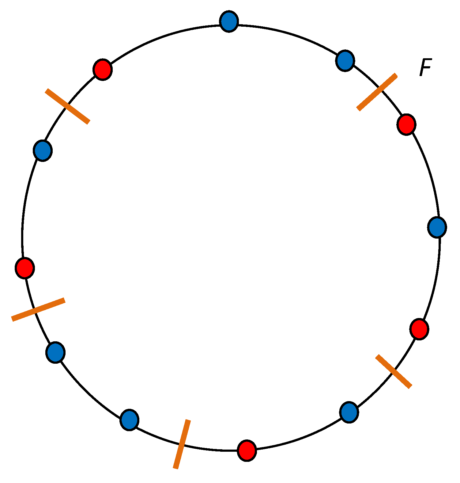
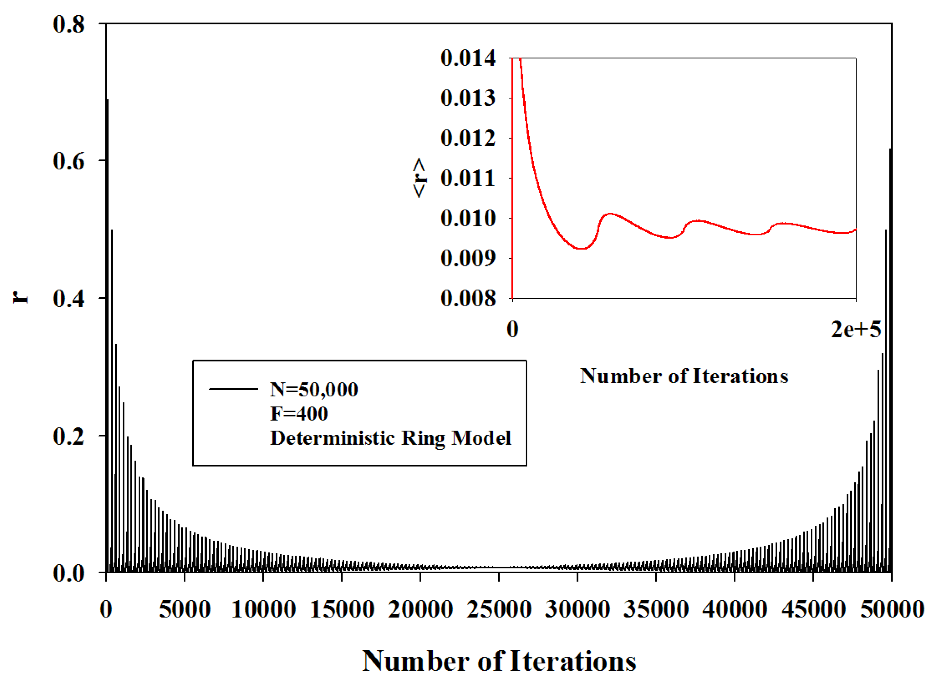
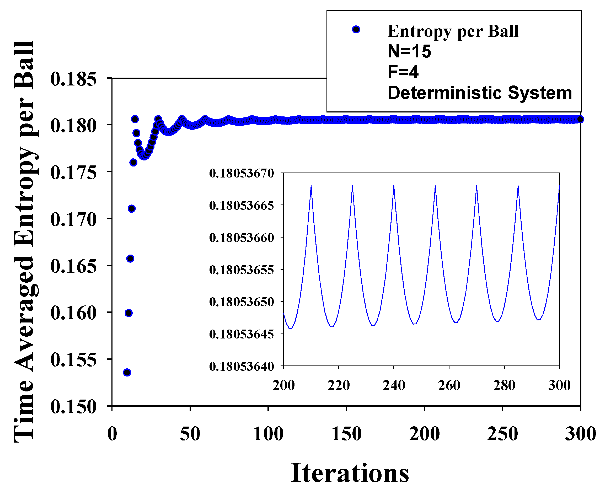
6.1. Lack of Molecular Chaos: Kac Ring Model

To understand how deterministic dynamics fails to describe a non-equilibrium system, we consider Kac’s ring model [65,66,67] containing N balls of two colors, red (A) and blue (B); see Figure 4. One can think of the balls as Ising spins $S=\pm 1$, with $S=+1$ representing red balls (A) and $S=-1$ representing blue balls (B). The N balls are localized on sites of the ring; there are no empty sites. These sites are equi-distant and cover the entire ring. A microstate i represents an ordered sequence of the colors of the balls, which we take to be clockwise starting from the top of the ring. The time evolution occurs by balls moving in unison one step (a rotation by $360{}^{\circ }/N$) clockwise during each time interval $\delta$. To include the environmental effects, we consider F flippers with fixed positions on the links between neighboring sites. The flippers flip the colors of balls (A⇔B) with certainty and without any bias as they pass through the flippers. The movement of each ball is deterministic, even when it passes through a flipper. In one time step, the microstate j evolves into another unique microstate $j^{\prime }$: we have a one-to-one mapping $j\to j^{\prime }$, which can be inverted to give the backward evolution $j^{\prime }\to j$ under time reversal ($t\to -t$) by balls moving counter-clockwise; there is no effect on flippers’ ability to flip colors under reversal. The system is time-reversal invariant. The number of distinct microstates of balls is $W=2^N$. For very weak external interactions, we need the flipper density $\phi \equiv F/N\ll 1$. Let $A_k$ and $B_k$denote the number of A and B balls and $a_k$ and $b_k$the number of A and B balls with a flipper ahead of them at time $t_k=k\delta .$ Obviously,

$$A_k+B_k\equiv N,a_k+b_k\equiv F$$

so that we can treat only one species (we choose B) as independent. It is easy to establish the following recursion relation [65,67]

$$B_{k+1}\equiv B_k+a_k-b_k$$

(29)

Introducing the densities $P_k=B_k/N$ and $p_k=b_k/F,$ we can rewrite the recursion relation for $P_k$:

$$P_{k+1}\equiv P_k+\phi (1-2p_k)$$

(30)

This recursion relation cannot be solved in a closed form, since it involves the quantity $p_k$ which is determined by the initial microstate and k. To proceed further analytically, we need to supplemented it by some known form of $p_k$. The most direct way is to express $p_k$ as a function of $P_k$. One such choice, following Burbury [27] and Boltzmann [22,23], is that of molecular chaos assumption (Stosszahlansatz, the collision number hypothesis) used in the kinetic theory of gases. According to this hypothesis, the velocities of colliding particles are uncorrelated, and independent of position. The hypothesis allows for establishing the famous H-theorem [22,23]. For the current model, in which the role of collisions is played by changing of colors due to flippers, it corresponds to [65,67]

$$p_k\equiv P_k$$

(31)

the density of any color is independent of whether a flipper is ahead or not. In other words, the presence of flippers has no effect on the densities of the balls of either color. This condition reduces to

$$r_k\equiv b_k/B_k=F/N$$

(32)

The recursion relation now becomes

$$P_{k+1}\equiv P_k(1-2\phi )+\phi$$

and can be solved recursively to obtain the limiting value $P_{\mathrm{eq}}$ of $P_k$ as $k\to \infty$, which represents the fix-point of the relation. At the fix-point, $P_{k+1}\equiv P_k=$ $P_{\mathrm{eq}}$, so that the second term in (30) must vanish. We clearly see that

$$P_{\mathrm{eq}}=1/2$$

(33)

at the fix point, regardless of the value of $\phi >0$ [65,66,67]. The fix point is independent of the choice of $\phi >0$ and also the initial value $P_1$. As there is no memory of the initial state or the density of flippers, the fix point must represents the equilibrium state in which half the balls are red, the other half blue. Thus, we come to the important conclusion that a deterministic dynamics along with the assumption of molecular chaos results in a very simple manner the equilibrium state at the end [68]. This is a remarkable result, and points to the deep insight of Boltzmann.

We were careful in not allowing $\phi =0$ in the above conclusion, since in this case, the recursion relation becomes trivial: $P_{k+1}\equiv P_k$. The initial state in terms of $P_1$ persists forever, as there is no dynamics to change the colors of balls anymore. Thus, the molecular chaos assumption requires a non-zero $\phi$, no matter how small.

The question that naturally arises is the following: Is the assumption of molecular assumption independent of the deterministic dynamics, or a consequence of it for a macroscopic system? As we know, the recurrence in a deterministic dynamics will ensure that the ratio $r_k$ will also recur after the passage of each recurrence time $t_{\mathrm{R}}$. During each recurrence, the variation of the ratio $r_k$ will follow exactly the same pattern as during the first recurrence. In other words, there is no possibility that the ratio will ever reach any limiting value, equal to the right hand side in (32). Even the iteration average $<r{>}_n$

$$<r{>}_n\equiv \frac{1}{n}\sum _{k=1}^n{r}_k$$

of $r_k$ over $n\ge 1$ iterations will have the same value $<r_N>$ at the end of each recurrence cycle (n an integer multiple of N). We only show r over the first Poincaré cycle is shown as a function of the iteration number n in Figure 5; however, the recurring pattern of the iteration average is shown in the inset for the first 14 recurrence cycles as a function of n. We have considered $N=\mathrm{50,000}$ balls, and $F=400$ equi-distant flippers, so that the right side in (32) is $0.008$, which is the lowest value on the ordinate in the inset. The initial state corresponds all balls blue. We clearly see the oscillations in the average $<r>$, as expected. However, theses oscillations are about a value very different from $0.008$. It is clear, therefore, that even with such large numbers of balls, there is no possibility for the molecular chaos assumption to be satisfied. The molecular chaos does not follow from the deterministic Kac’s ring model [69].

As the molecular chaos assumption is needed for the validation of the H-theorem, or the second law, we can conclude that a deterministic dynamics alone cannot lead to the second law. Moreover, as the assumption of molecular chaos is not satisfied, the recursion relation will not approach its fix point solution so that equilibrium will not occur if we only follow the deterministic dynamics. This is because the initial state recurs over and over again after its Poincaré cycle, as expected from Poincaré’s recurrence theorem (1) [70].

It should be observed that we have only cast doubt on the lack of molecular chaos in Kac’s deterministic ring model. However, a single counterexample, Kac’s ring model, is sufficient to prove the that molecular chaos is not a consequence of a deterministic dynamics.

6.2. Zermelo’s Incorrect Conclusion

During any later recurrence period, the microstates again evolve following the cycle (28), so that the probabilities first become different from $p=1/W$, only to become $p=1/W$ at the end of each cycle. Consequently, the temporal entropy will decrease from $lnW$ and rise again to this value in a cyclic manner; it will, however, never become zero; see below. Let us again consider Kac’s ring model [65,66,67]; see Figure 4. It is easy to see that the recurrence time is the time required for one complete rotation if F is even, or two complete rotations if F is odd. An iteration is said to occur when the ring has gone through a rotation by $2\pi /N$. Thus, N iterations are required for one rotation of the ring. We perform a large number of iterations [69] and calculate the temporal entropy, which is reported in Figure 6 for $N=15,F=4$. The initial microstate has all balls red. The recurrence cycle for this microstate is 15 iterations, or one rotation of the ring [69]. We see that the entropy reaches its maximum at integer multiples of 15 for the number of iterations. However, after the first cycle, the entropy undergoes oscillations, whose depth relative to the recurring maximum decreases with the number of recurrences. In the inset, we show these oscillations at higher end of the iterations. We find that the oscillations have not died out, although their depths are very slowly decaying to zero. What we also notice is that the entropy does not revert to its original entropy, as claimed by Zermelo [35,36], even though the entropy does decrease, as argued by him.

Notice that the maximum entropy per ball is not equal to $ln2$; rather it is

$$S_{\max }/N=ln(15)/15\simeq 0.1805$$

(34)

This is because the initial state belongs to a disjoint component with 15 microstates. Thus, the system cannot leave this component. This is an example in which the temporal entropy gives a value which is not the maximum possible value. The latter will usually happens when the system gets trapped in a disjoint component in the phase space.

Theorem 4

The temporal entropy $S(t)$ periodically achieves its maximum allowed value $lnW$ at the end of each Poincaré cycle, and in-between two successive cycles, it has a minimum value whose depth decreases with the order $n=2,3,\cdots$ of the cycle but is independent of N. However, the magnitudes of these drops for the entropy per particle $s(t)\equiv S(t)/N$ vanish as $N\to \infty$ for all n, so that oscillations in the entropy per particle $s(t)$ disappear and the second law remains intact in terms of $s(t)$. As a consequence, Zermelo’s paradox disappears for a macroscopic system.

Proof. 

We now consider a general situation for such oscillations in an arbitrary system with deterministic dynamics and consider the nth Poincaré cycle, $n=2,3,\cdots$. At the end of the last $(n-1)$th cycle, all microstates have occurred $n^{\prime }\equiv n-1$ times. Let us consider the situation at some intermediate time during the nth recurrence cycle, and let $j_0,j_1,j_2,\cdots ,j_k$, $k<W-1$ denote the microstates that have appeared n times, while the rest of the $W-k$ microstates have only occurred $n^{\prime }$ times. The temporal entropy is now given by

$$\begin{array}{cc}\hfill S_n(t)& =-k[n/(n^{\prime }W+k)]ln[n/(n^{\prime }W+k)]\hfill \\ & -(W-k)[n^{\prime }/(n^{\prime }W+k)]ln[n^{\prime }/(n^{\prime }W+k)]\hfill \\ & =ln(W+\frac{k}{n^{\prime }})-\frac{nk}{(n^{\prime }W+k)}ln\frac{n}{n^{\prime }}\hfill \\ & =lnW+ln(1+\kappa )-\frac{n\kappa }{(1+\kappa )}ln\frac{n}{n^{\prime }},\hfill \end{array}$$

where $t=t_{\mathrm{R}}+k\delta$, and where $\kappa \equiv k/n^{\prime }W$. We see that for $n^{\prime }\kappa =1$, which means that $k=W$, the entropy is exactly $lnW$. We have already seen in the previous section that the temporal entropy has this value at the first recurrence. Thus, the temporal entropy has the same value $lnW$ at each recurrence. This proves the first part of the theorem.

The difference of the minimum entropy from the maximum entropy in the nth cycle is

$$\Delta S_n\equiv S_n(t)-lnW=ln(1+\kappa )-\frac{n\kappa }{(1+\kappa )}ln\frac{n}{n^{\prime }}$$

For a macroscopic system ($N>>1$), we can treat $\kappa$ as a continuous variable so that the entropy becomes a continuous function of $\kappa$. Let us differentiate it with respect to $\kappa$ to obtain

$$\frac{d{S}_n}{d\kappa }=\frac{1}{(1+\kappa )}-\frac{n}{{(1+\kappa )}^2}ln\frac{n}{n^{\prime }}$$

which vanishes for

$$1+\kappa =nln\frac{n}{n^{\prime }}$$

Thus, the difference in the maximum and minimum entropies in the nth cycle is

$$\Delta S_n=-(nln\frac{n}{n^{\prime }}-1)+ln(nln\frac{n}{n^{\prime }})<0$$

regardless of the number of particles N. For $n=2$, we find that $\Delta S_2\approx -0.05966$. One should compare this difference with the difference we observe during the second cycle in Figure 6. Thus, the temporal entropy violates the second law due to these oscillations.

This drop in the entropy vanishes in the thermodynamic limit $N\to \infty$ if we consider the entropy difference per particle

$$\frac{\Delta S_n}{N}\stackrel{N\to \infty }{\to }0$$

(35)

Thus, the recurrence has no effect on the entropy per particle in the thermodynamic limit. It remains equal to the maximum entropy per particle $\left[=(1/N)lnW\right]$. One can easily extend the above calculation to higher cycles, with the same conclusion that the entropy S shows oscillations even in higher cycles, so that the temporal entropy will violate the second law. However, the entropy per particle does not show any deviation from the second law as in the second cycle shown above. This shows that Zermelo’s conclusion is incorrect if we consider the entropy per particle $S/N$. If we consider the entropy S, then there are oscillations in the temporal entropy, but the amplitude of these oscillations are bounded, independent of N. In this regard, Zermelo’s objection to Boltzmann’s law of increase of entropy is partially valid. However, his objection is partially invalid in that the oscillations will not bring the entropy back to its initial value. Zermelo’s conclusion was incorrect. Let us evaluate the slope $dS/d\kappa$ at $\kappa \to 0^{+}$:

$${\left.\frac{d{S}_n}{d\kappa }\right|}_{\kappa \to 0^{+}}\to 1-nln\frac{n}{n^{\prime }}.\approx -0.3863.$$

For $n=2$, this derivative is $\approx -0.3863.$ As $k\delta =\Delta t\equiv t-t_{\mathrm{R}},$ we find that

$$W\delta {\left.\frac{d{S}_n}{dt}\right|}_{t\to t_{\mathrm{R}}^{+}}\equiv {\left.\frac{d{S}_n}{d\kappa }\right|}_{\kappa \to 0^{+}}$$

thus, the slope for a macroscopic system ($N\to \infty$) vanishes

$${\left.\frac{d{S}_n}{dt}\right|}_{t\to t_{\mathrm{R}}^{+}}\to 0$$

One can easily check that the slope also vanishes as $t\to n{t}_{\mathrm{R}}^{-}.$ Thus, the slope $d{S}_n/dt$ vanishes at $t=t_{\mathrm{R}}$, a property expected of a continuous function at its maximum. ⏹

Moreover, the ensemble and temporal entropies are not different if the dynamics allows all the states to be visited during a cycle. This is obviously not true if the system gets confined to a component of the phase space, as is the case with the ring model studied above.

7. Stochastic Dynamics

7.1. Lessons from Kac’s Ring Model

7.1.1. Need for Stochasticity

Now that we have seen that molecular chaos is not a consequence of the temporal reversibility present in a deterministic dynamics, we need to look for a much deeper cause of irreversibility. This is precisely the argument that was put forward by Loschmidt [25] against the proof of the H-theorem by Boltzmann [22,23]. Following Kröning [26], Boltzmann [23], Burbury [27], and Landau [45] among others, we propose that it is the stochastic nature of a statistical system that is responsible for time irreversibility [38]. While the idea of a stochastic approach to a statistical system is not new, we hope that our main contribution is to clarify its source in the form of stochastic interactions with the medium, which results in a stochastic dynamics of the microstates. This should be contrasted with the dynamics of the macrostate or thermodynamic averages. Usually, such dynamics are described by the Langevin equation or the Fokker-Planck equation [9]. The central idea here is that the collisions between particles give rise to fluctuating stochastic forces. However, as the collisions are described by the potentials in the Hamiltonian, they cannot by themselves be sources of stochasticity [64]. In our view, it is the stochastic interactions with the medium that results in a haphazard motion of the particles, which in turn make the collisions among them stochastic everywhere inside the system. This will be clearly seen in the example discussed in Section 8. Thus, we will adopt the view here that the microstates evolve stochastically in time. The presence of these stochastic interactions with the medium, the latter corresponding to the extra degrees of freedom $\psi (t)$, immediately invalidates the time reversal invariance. At present, it appears to be prima facie an ad-hoc assumption, but its reliance is based on physical intuition and a posteriori justification by the success of the assumption. We now justify this proposal.

For the concept of entropy to be useful requires a particular kind of probabilistic approach in which the evolution must not be deterministic, even though one can use densities such as $P_k$ above for a deterministic system as a suggestive probability; rather, it must be genuinely $stochastic$. As Landau observes [45], even an isolated system is not truly deterministic in Nature. A real system must be confined by a real container, which forms the exterior of the system. The container cannot be a perfect insulator. Moreover, it itself will introduce environmental noise in the system. Thus, there are always stochastic disturbances going on in a real system due to the exterior, which cannot be eliminated, though they can be minimized. (For the Kac ring model, we must ensure $\phi \ll 1$, but we must not have $\phi \equiv 0$, as discussed above; in the latter case, the dynamics is absent. The absence of a dynamics is a special kind of a deterministic evolution, so that the entropy will remain constant.) For quantum systems, this requires considering the Landau-von Neumann density matrix, rather than eigenstates [45]. The derivation in [45] clearly shows the uncertainty introduced by the presence of “outside,” the medium. The latter is not part of the system, just as the flippers are not; recall that the flippers are not used in identifying the microstates and their density does not affect the fix point (33) [68]. This is also the situation with the extra degrees of freedom $\psi (t)$ in $\{\varphi (t),\psi (t)\}$ introduced in Section 1.5, which are not part of the system.

7.1.2. $P_{k+1}$ ↛ $P_k$ under Time-reversal

We do not have to consider the actual nature of the noise; all that is required is its mere presence. One can think of $\phi$ in the Kac model as a measure of the strength of stochastic noise; see Gujrati [68]. For this, we change the deterministic Kac model to a stochastic model by introducing stochasticity: We make the flippers change the colors randomly with a probability p to mimic stochastic external interactions. There are other versions of the stochastic ring model discussed by Gujrati [68]. We will here consider the above simplified model. It is easier to focus on one particular ball and follow its evolution. Let $P_k$ denote the probability that this ball is blue and $p_k$ (or $1-p_k$) the probability that the ball ahead of a flipper is blue (or red) at the kth iteration. The probability $P_{k+1}$ at the next iteration is given by considering the probability $p\phi (1-p_k)$ that a red ball ahead of the flipper is turned blue and the probabillity $p\phi p_k$ that a blue ball is turned red:

$$P_{k+1}=P_k+p\phi (1-p_k)-p\phi p_k$$

(36)

As a consequence, (30) is replaced by

$$P_{k+1}\equiv P_k+p\phi (1-2p_k)$$

(37)

We do not assume (31) or (32) so that we can test if the molecular chaos condition emerges automatically out of the stochastic dynamics. The fix point of (37) occurs when

$$p_k=1/2$$

This, however, does not determine the value of $P_k$ as $k\to \infty$. Therefore, the above recursion relation is not useful in determining the equilibrium value of $P_{\infty }$. It cannot be iterated as it requires knowing $p_k$. Instead, we start with an initial state, which we take to be all balls blue and fix the locations of the flippers equidistant on the links. Thus, $B_0=N$ and $b_0=F$, assuming that all the flippers are present. We then turn the ring by $360{}^{\circ }/N$ for the next iteration clockwise and change the colors of the balls with probability $p$when they pass through the flippers. We determine $b_1$ and $B_1$ and compute their ratio $r_1\equiv b_1/B_1$ at each iteration. We then perform the next iteration and so on. At each iteration, we determine $b_k,B_k$ and their ratio $r_k\equiv b_k/B_k$. The recursion relation (29) is replaced by the following recursion relation

$$B_{k+1}=B_k+p(a_k-b_k)$$

(38)

at each iteration. If we now introduce ${\widehat{P}}_k\equiv B_k/N$ and ${\widehat{p}}_k\equiv b_k/N$, we can rewrite (38) in the form

$${\widehat{P}}_{k+1}={\widehat{P}}_k+p\phi (1-2{\widehat{p}}_k)$$

which, not surprisingly, is identical in appearace to (37) and modifies (30) to the staochastic case.

We have considered a small system with $N=\mathrm{1,000}$ and $F=400$, and have iterated $\mathrm{700,000}$ times that is more than sufficient to reach equilibrium. We find that $P_k$→$1/2$, as well as $p_k$→$1/2$, as expected. We show the result for the raio $r_k$ for the later iterations in Figure 7. We find that (32) is found to be satisfied after a large number of iterations. While $r_k$ undergoes random jumps, its average over a long time is identical to the flipper density $\phi =.01,$ as shown by the horizontal line in the figure. It is clear now that the molecular chaos assumption is really a consequence of our stochastic model analog. One no longer has to make the molecular chaos assumption separately.

As long as $p\phi \ne 0$, the model will always converge to the fix point, i.e. will equilibrate in an average sense. It is only in this case that the entropy will increase as the probabilities of various microstates change in time. The actual nature of the noise will only determine the form of the dynamics, but not the final equilibrium state, which remains oblivious to the actual noise or the dynamics. This is what allows the statistical mechanical approach to make predictions about the equilibrium state. Since the evolution is stochastic, a microstate j makes a “jump” to one of the W microstates in the microstate set $\left\{J\right\}$. The mapping

$$j⤏\left\{J\right\}$$

is one-to-many, with each of the possible $j^{\prime }\in \left\{J\right\}$ occurring with some probability. Because of the one-to-many nature, the mapping cannot be inverted to study time-reversal, and strict causality is destroyed. To appreciate this observation, let us consider the Kac ring model. Under time-reversal, the balls move counter-clockwise, but flippers continue to flip colors with the same probability p. Thus, $j^{\prime }$ gives rise to two possibilities so the mapping still remains one-to-many, which causes irreversibility: $P_{k+1}$ does not go back to $P_k$; it goes to $P_{k+2},$ as if time has not reversed.

7.1.3. Effect of Time Reversal on the Entropy

Based on the above observation, we now follow the consequence of time reversal on the entropy. Let us reverse time at $t=t_0>0$, where the entropy is $S(t_0);$ see Figure 2. Then all possible microstate in the set $\left\{J\right\}$ will not uniquely jump back into $j;$ rather each of the possible $j^{\prime }$ will stochastically jump to any of the W microstates in the set $\left\{J\right\}$, and the entropy will continue to increase from its value $S(t_0)$. This is shown by O${}_0$C in Figure 2. The entropy will not follow O${}_0$O. However, O${}_0$C is the “mirror-image” of O${}_0$A in a “mirror” located at $t=t_0$. This is the time-reversal invariance of the entropy at $t_0>0$. The situation is the same at $t=0,$ when the system was initially prepared in some non-equilibrium state. If we follow its evolution in past and in future separately, we will discover that the entropy continues to increase until equilibrium is reached in both cases; see OA and OB in Figure 2; both are “mirror-images” of each other in a “mirror” located at $t=0$. Thus, time-reversal invariance is intact as far as the entropy is concerned, regardless of t. Thus, with the stochastic dynamics, the temporal symmetry and homogeneity appears in the behavior of the entropy. This is quite remarkable.

7.1.4. Idealized walls

Idealized walls are walls that result in elastic collisions when a gas molecule strikes. In this case, the kinetic energy does not change so that it remains a constant of motion. Ideal gases confined by idealized walls to form isolated systems have no mechanism to achieve equilibrium, and will remain in non-equilibrium states for ever if they were so initially; see footnote 6 in [30]. This also remains true if the system is in a medium with a fixed pressure. Then, it follows from the virial theorem [45] that for an ideal gas

$$3PV=2K$$

where K does not have to be equal to $3NT/2$ (monatomic gas particles), unless the gas is in equilibrium. We have already discussed earlier in Section 5.3 that the entropy in a deterministic dynamics does not approach equilibrium, unless the system is already in equilibrium; the system retains the memory of the initial state. For the concept of entropy to be useful requires it to be an intrinsic property of the system so that it is not affected by the measurements used to prepare the initial state if we wait long enough after the measurements. Thus, the concept of entropy requires a particular kind of probabilistic approach in which the evolution must not be deterministic; rather, it must be $stochastic$. Even an isolated system is not truly deterministic in Nature. A real system must be confined by a real container, which cannot be a perfect insulator. Even the container will introduce environmental noise in the system, a point made many times in the literature; see for example Hoover [71] for an equivalent statement in point (iv) while discussing reversibility of Newton’s equation. Thus, there are always stochastic processes going on in a real system, which cannot be eliminated, though they can be minimized. In the case the external noise is too strong, then there is no sense in not considering the environment as part of the system for its thermodynamic investigation. It is the limit in which the external noise is too weak that is relevant for a sensible thermodynamical description of a system, so that the external noise will not alter the average properties such as the average energy of the system [68].

7.1.5. Real Systems

A real system will always have stochastic interactions with the surroundings that will result in transitions among microstates so that eventually we lose information about the initial microstates $j_k$ as they evolve in time and eventually the entropy reaches its maximum value of $lnW$ that the system had just before the microstate measurement. What the above discussion, especially regarding the temporal entropy, illustrates is the importance of stochastic interactions, no matter how weak, with the surroundings [62] in inducing transitions among microstates so that the behavior of the system becomes consistent with the second law. There is no Poincaré recurrence now. Without any stochasticity, the evolution of the system becomes deterministic for which the ensemble entropy remains constant [62] as discussed above, but the temporal entropy usually oscillates. Therefore, in the following, we will always consider the evolution of a system to be stochastic, unless noted otherwise.

7.2. One-to-many Mapping of Microstates, Temporal Asymmetry, and Entropy Change

The stochasticity introduces a new time scale $\Delta$ over which the system evolves deterministically as above. Over this time-period, the the mapping $j\to j_k$ is one-to-one so that the entropy remains constant during this period. At the end of each time period $\Delta$, i.e. at time $t=t_k^{\prime }\equiv k$$\Delta ,k=1,2,\cdots$, the current microstate j will undergo a stochastic “jump” ( shown by the broken arrow $j⤏j^{\prime }$) to any of the W microstates $j^{\prime }$ [72] brought about by the environmental noise. We take these “jumps” to occur instantaneously just for simplicity. This will then mean that $\Delta =\delta$, the time introduced earlier for a microstate to evolve into a different microstate. This also means that $t_k^{\prime }=t_k$ introduced earlier. The “jump” may create a new microstate not generated so far, or bring it back to a previously generated microstate, including the initial microstate. Such a jump to a previously generated microstate (not the initial microstate) would have been forbidden in a deterministic evolution alone as noted above. Many such stochastic “jumps” are needed to bring the system to equilibrium, which requires a time interval $t_{\mathrm{eq}}$, so that $\delta <<t_{\mathrm{eq}}$. The presence of stochastic “jumps” gives rise to a probabilistic nature to the microstates, their probability of occurrence changing with time. This in turn changes the entropy with time whenever “jumps” occur [68].

The final equilibrium state remains oblivious to the actual noise. This is what allows the statistical mechanical approach to make predictions about the equilibrium state. We consider an ensemble of $\mathcal{N}$ replicas, each replica being identically prepared in the same microstate 0 at time $t=0$, so that $p_j(0)={\delta }_{j0}$. Consequently, $S(0)=0$. This obviously represents an extreme non-equilibrium situation. However, since the evolution is stochastic, a microstate j makes a “jump” to another microstate $j^{\prime }$ ($j⤏j^{\prime }$) or remain the same ($j⤏j$) caused by the noise. It is also possible to have $j⤏j^{\prime }⤏j$, as shown in Figure 3b, where we show that the system leaves the original microstate 0 but comes back to it at $t_k$. Thus, the recurrence can happen at any time $t\ge \delta$, albeit without certainty (probability $p_0(t)<1$) [73] and has no particular significance or relevance for the Poincaré cycle for a finite but macroscopic system, where recurrence occurs with certainty. This distinction in the probability of recurrence is very important, as the entropy is determined by the probability. Just because the initial microstate has recurred does not necessarily mean that the entropy has reversed to its initial value $S(0)=0$, contrary to the claim by Zermelo. One needs to consider its probability also. To establish this, we proceed as follows.

At $t_1,$ there will be $\mathcal{N}{p}_j(t_1)$ replicas in the jth microstates. In particular, there is a non-zero probability $p_0(t_1)<1$ that the system will remain in its original microstate 0. However, this in no way means that $S(t_1)$ has reduced to zero, as it is obtained by (13), which requires a sum over all microstates that are present in the ensemble. The degree of uncertainty of the initial microstate

$$u_0(t_1)=-ln{p}_0(t_1)>0$$

so that $S(t_1)>p_0(t_1)u_0(t_1)>0$. The entropy has increased. For $t_1<t<t_2,$ each replica evolves deterministically so that the entropy remains constant, as follows from Theorem 2. This is true during each of the intervals $t_k<t<t_{k+1},$ with the entropy changing at $t_k$ as the probabilities $p_i(t_k)$ change. During all this time, the system has a non-zero probability $p_0(t)<1$ to be in the initial microstate 0. Eventually, the system equilibrates when (18) holds so that ($W^{\prime }=W-1$)

$$u_j(t)\to lnW,j=0,1,\cdots ,W^{\prime }$$

which is exactly the entropy $S(t)=lnW$ of the system obtained by summing over all microstates; see (17). We observe that in equilibrium, the entropy is exactly the degree of uncertainty of any microstate and, in particular, the initial state.

Thus, we come to the following theorem:

Theorem 5

Even for a stochastic evolution, which is needed for a statistical system, the recurrence of the initial microstate does not violate the second law.

The entropy remains constant after equilibrium is reached. The recurrence of the initial microstate 0 (but with $p_0(t)=1/W$) in the stochastic case does not mean that the entropy reverts to the initial entropy $S(0).$On the other hand, the true recurrence of the initial microstate 0 $\left[p_0(0)=1,S(0)=0\right]$ requires $p_0(t)=1$, for which all replicas must be in the microstate 0 simultaneously. This can occur in only one way. However, such a true recurrence is impossible in stochastic systems. To show this, we consider the situation in equilibrium; see (18). The number of possible ways the replicas can be arranged at time t, consistent with microstate probabilities $p_i(t)$, is

$$\mathcal{N}!/\prod \left[\mathcal{N}{p}_i(t)\right]!\approx e^{\mathcal{N}S(t)}=W^{\mathcal{N}}$$

(39)

one of which is the true recurrent state. Hence, the probability for the initial microstate to truly recur is $W^{-\mathcal{N}}\to 0$ as $\mathcal{N}\to \infty$. The recurrence of 0 occurs [32,37] several times, but with $p_0(t)<1$, so that other microstates have to be considered to determine $S(t)$.

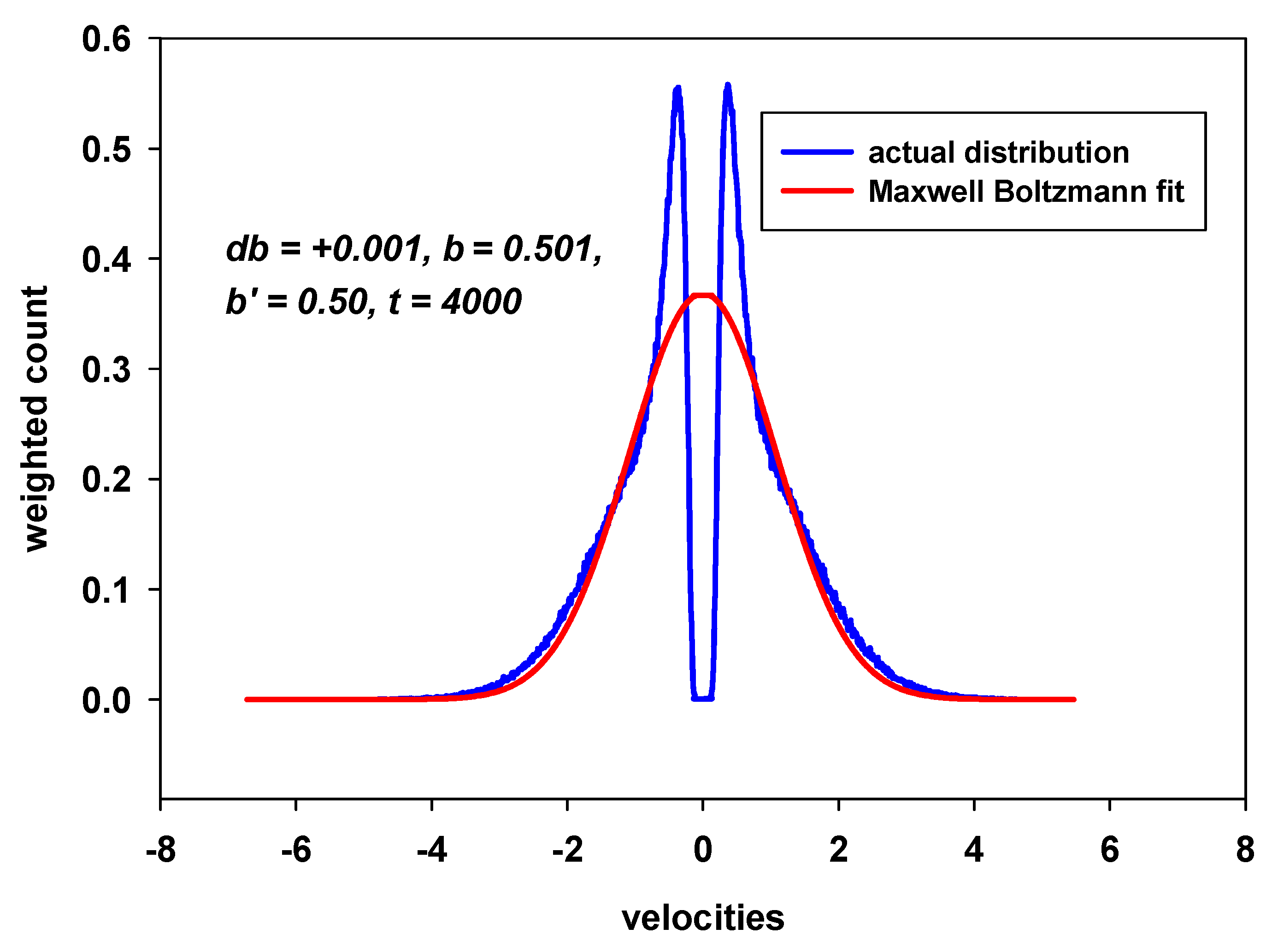
8. Stochastic Impulses from the Walls: 1-d Ideal Gas

8.1. Reconstruction of Walls and Stochastic Impulses

At any non-zero temperature of the surrounding medium, the atoms or molecules making up the walls of the container in which the system is contained continue to undergo reconstruction due to thermal fluctuations. Even at absolute zero, they experience zero-point vibrations. However, in this work, we will neglect quantum fluctuations. The reconstruction results in changing the positions of these particles in the walls in time. Accordingly, the walls cannot be taken as static as the system approaches towards equilibrium. Every time a particle of the system collides with the walls, it finds the walls in different states than at earlier times. Moreover, since thermal effects on the walls are random, the walls become the source of stochastic actions on the particles of the system.

Let us consider an ideal gas with N non-interacting identical particles, confined inside a 1-d box of length L. The walls of the box are at $x=0$ and $x=L$. We will also assume that the collisions between particles are completely elastic. It is well known from classical mechanics that if two particles of identical mass elastically collide, they merely interchange their velocities. If $v_1$ and $v_2$ are the velocities before collision, and $v_1^{\prime }$ and $v_2^{\prime }$ are the velocities after collision, then

$$v_1^{\prime }=v_2,v_2^{\prime }=v_1$$

Thus, if we take into account the identical nature of the particles, and interchange their labels after the collision, we have as if the particles never experienced any elastic collision, but continued to follow their course. If a particle is moving to the right with a velocity v before collision, a particle is again moving to the right with the same velocity v. Therefore, the collisions between particles can be forgotten for identical particles. We only need to worry about the walls at the two ends. We assume that every time a particle collides with a wall, it imparts a random impulse to the particle so that not only its direction is reversed, but also the magnitude of its momentum undergoes a random change. We will assume the mass m of each particle to be arbitrarily set to $m=1.$ Similarly, we will arbitrarily set $L=1,$ so that we do not have to keep track of these quantities in our calculation. The initial velocity is taken to be $v_0=1,$ and the particle is initially located at $x=0$. At each collision with a wall, we have

$$v\to v^{\prime }=-v(1+\eta b(\eta ))$$

where $\eta$ is a random variable between $(-1,+1)$ with a certain time-independent probability distribution $P(\eta )$, and b measures the effect of the random impulse. Also, for simplicity, we only consider the simple case of

$$P(+1)=P(-1)=1/2$$

8.2. Average Kinetic Energy

Let us consider the possible velocities at the nth collision, each with a probability ${(1/2)}^n$. These velocities are given by

$${(-1)}^n{(1+b)}^k{(1-b^{\prime })}^{n-k}$$

with $k=0,1,\cdots ,n$., and where $b_1=b(+1),b_1^{\prime }=b(-1)$. The number of times these velocities occur is given by

$$\left(\begin{array}{c}n\\ k\end{array}\right)$$

Thus, the average kinetic energy ${\overline{K}}_n$ at the nth collision is given by

$$2{\overline{K}}_n=\frac{1}{2^n}\sum _k\left(\begin{array}{c}n\\ k\end{array}\right){(1+b_1)}^{2k}{(1-b_1^{\prime })}^{2(n-k)}={\left[1+\Delta b_{12}+\overline{b_{12}^2}\right]}^n$$

where

$$\Delta b_{12}\equiv b_1-b_1^{\prime },\overline{b_{12}^2}\equiv \frac{1}{2}(b_1^2+b_1^{\prime 2})$$

To ensure that the average kinetic energy remains bounded, we can take [74]

$$b_1=b/n,b_1=b^{\prime }/n$$

In this case,

$$2{\overline{K}}_n\stackrel{n\to \infty }{\to }exp(\Delta b)$$

where

$$\Delta b=b-b^{\prime }$$

In the 1-d case, the average kinetic energy from the law of equipartition is $T/2$, where T is the temperature in the units of the Boltzmann constant. Assuming the equipartition is a valid assumption, we have

$$T=exp(\Delta b)$$

8.3. Temporal Inhomogeneity

We should comment on the choice of the variation of the impulse with the number of collisions. Since the stochastic impulse depends on n, its magnitude depends on the history. Moreover, the strength of the impulse at a certain collision n will change if we shift n by a constant, in analogy with (2). Thus, the temporal homogeneity has been lost by the above choice of the random impulse. This is in addition to the loss of temporal symmetry due to the stochastic nature of the impulse. Thus, since the temporal symmetry is already lost, the temporal inhomogeneity has no additional consequence.

8.4. Some Results

We will only present some selected results from our computation here [74].

The discussion above is valid only as $n\to \infty$. However, not all velocities that appear at the nth collision occur at the same time. Indeed, the time at which a certain velocity occurs depends on the entire history of the intermediate velocities since $t=0$. Thus, we need to find all the velocities that have appeared at a given time t. This problem cannot be solved analytically. Our computation has been carried out with the $L=1$, and $v(t=0)=1$. The unit of time is given by $L/v(t=0)$, in terms of which t becomes dimensionless. Indeed, even the velocity in terms of $v(t=0)$ is dimensionless. We also take the mass of the particle to be $m=1$. We have carried our numerical simulations up to $t=4000$. The averages such as $\overline{K}$ and S reported here are ensemble averages.

In Figure 9, we show $\overline{K}$ as a function of t for three different choices of the parameters. We see that $\overline{K}$ has not reached its equilibrium value for the top curve, while equilibrium has been achieved for the lower two curves. This shows that the time $t_{\mathrm{eq}}$ depends on the set of parameters. A higher value of $\Delta b$ at a fixed $b^{\prime }$ gives rise to a higher average kinetic energy or temperature. Thus, the simple model possesses the characteristic of approach to equilibrium. The corresponding temperatures from top to bottom are $T=1.614,1.48,$ and $1.466$.

In Figure 10, we compare the velocity distribution at $t=4000$ with the expected Maxwell distribution. We observe that there is a gap in the numerical distribution neat $v=0$. The reason for this is obvious. One must wait for an infinite number of collisions ($n\to \infty$) to obtain $v=0$. We have checked [74], but do not report here, that the gap near the origin decrease as t increases. However, the effect is very slow. The Maxwell distribution is drawn so that the area under the two curves are the same. We can obtain an independent estimate of the temperature from this Maxwell distribution. For the situation shown in Figure 10, this estimate of the mperature is $T=1.34,$ which should be compared with $T=$$1.48$ obtained from the average kinetic energy in Figure 9. The discrepancy between the two values is presumably with the uncertainty in fitting the Maxwell distribution. This is under investigation at present.

In Figure 11, we plot the ensemble entropy due to the velocities as a function of time. We do not report the part of the entropy determined by the positions of the particles. We see that the entropies for the three sets of parameters reach their maximum values rather fast for these parameters. We see how the entropies satisfy the second law because of the presence of stochasticity at the walls. The corresponding temperatures obtained from the average kinetic energies (results not presented here, but are given in [74]) are $T=0.61,0.69,$ and $0.81$, as we go from the lower to the higher curves. This behavior suggests that the entropy increases with the temperature, as expected from the entropy.

Thus, we see that the above simple model that introduces stochasticity at the walls is able to capture all the desirable features of thermodynamics. Idealized walls would not be able to capture these features.

9. Discussion and Conclusions

As noted by Prigogine, Grecos and George [20], “…Boltzmann’s derivation of his kinetic equation was basically phenomenological. The main step involved is the replacement of the dynamical laws by a physically plausible stochastic mechanism." It is this stochasticity that is the central theme of this review to bring about temporal asymmetry. In particular, close attention has been paid to the cause of this stochasticity and how this bring about temporal asymmetry and inhomogeneity. We have considered two alternative formulations of the entropy that appears in the second law or any thermodynamic average. The Fundamental Axiom proposed in Section 3 based on the additivity principle is taken to be the primary postulate to determine any thermodynamic average. Both, the ensemble and the temporal definitions of the average, which includes the entropy, require the same average over microstates. The only difference is in the form of the probability used for the microstates. Any difference between the two microstate probabilities results in a difference between the two averages. From our discussion, it is clear that the ensemble approach appears more fundamental than the temporal approach, because:

• The ensemble averages satisfy the additivity principle introduced in Section 3.
• The other reason is that most measurements last a short period of time. The temporal average over an extended time period has nothing to do with information obtained in measurements that may take a fraction of a second or so. In contrast, the ensemble average provides an instantaneous average and thus bypasses the objection of the finite measurement time.

The temporal average over a short period will only make sense if it remains equal to the ensemble average. This can only happen if the system was already in equilibrium to begin with. For non-equilibrium states, especially at low temperatures, its usefulness is quite questionable. Here, it may then take quite some time, much longer than the experimental time, before the temporal average can come close to the ensemble average. As the dynamics becomes too slow in the glassy state [60,61], this time may become astronomically large. Thus, temporal average may not be desirable in general. We refer to Tolman [53], Jaynes [57], and Becker [59], for additional information on this point.

Despite the lack of any real superiority of the temporal average, many people consider it to be of primary importance. Then, they need to justify its equivalence with the ensemble average, which then leads to the concept of ergodicity. It is important to mention that Gibbs himself did not find the concept of ergodicity relevant to the foundation of statistical mechanics, as it finds no place in his monumental work [52]. In our view, we should strive to ensure that the ensemble average is equal to the experimental values; see Fundamental Axiom. Whether the ensemble average is equal to the time average is of no use to an experimentalist since most experiments do not take that long to perform and, as has been known, see for example Jaynes [57], Huang [37] and Rice and Gray [54].

It should also be stressed that the temporal average over infinite time is most certainly inappropriate for glasses, which over a long period of time will relax to their equilibrium supercooled liquid states or to the ideal glass if left to themselves. Thus, the temporal average carried out over an infinitely long period will describe the equilibrated supercooled liquid or the ideal glass and not the glass, obtained under an experimental time constraint $t_{\mathrm{obs}}$. The ensemble average does not suffer from this problem, which therefore becomes the choice average to consider for studying glasses. We find that all the consequences of the ensemble approach remain consistent with the principles of thermodynamics. This is very important as the latter has been tested over and over again and found to be always valid.

We considered the applicability of the ensemble approach to systems confined in disjoint components in Section 4.3 and concluded that even here, one must average over all samples, and not restrict the calculation of any quantity such as the entropy over a single component.

Another aim of the revies was to investigate whether the second law is a consequence of a deterministic dynamics obeying temporal symmetry and homogeneity; see the above comment by Prigogine et. al. [20]. It is the original derivation of the H-theorem by Boltzmann [22,23,40,41] and the resulting controversies in the form of the recurrence paradox [35,36] and the irreversibility paradox [25] and their resolution that is the motivation behind this review. We find that the deterministic dynamics gives rise to a unique one-to-one evolution of microstates. Accordingly, the entropy in a Poincaré cycle remains constant. This constancy follows immediately from Liouville’s theorem in classical mechanics (or even in quantum mechanics, which we have not considered here), according to which the phase space density remains invariant. The constant entropy is equal to the Boltzmann entropy (17) only if the system is already in equilibrium. Thus, it is clear that a deterministic dynamics can never lead to the second law. In fact, if the system is not in equilibrium, no deterministic dynamics will lead to equilibration. This is exemplified by the results we present on Kac’s ring model. We find that if the dynamics in the model is deterministic, it does not lead to molecular chaos assumption used by Burbury [27], Boltzmann [23,40,41], and Maxwell [21]. Indeed, the Poincaré recurrence controls the tme evolution and ensures that all quantities behave cyclically. We considered the temporal evolution of the ratio $r_k$ in (32) over many Poincaré cycles, as shown in the inset in Figure 5. Surprisingly, the limiting value as the oscillations disappear is not close to the right hand side in (32). This counter-example is sufficient to disprove any suggestion or claim that the molecular chaos is a consequence of a deterministic dynamics in a system with large number of particles; we consider $N=50,000$ considered in this case to be large enough for us to draw this conclusion. On the other hand, if the dynamics in the ring model becomes stochastic, the molecular chaos emerges out of this dynamics; see Section 6.1 for details. We also find that the temporal entropy in a deterministic dynamics leads to an oscillatory behavior with a period equal to the Poincaré cycle. This was what Zermelo had pointed out [35,36]. But the temporal entropy does not revert back to the original value, which was also suggested by Zermelo [35,36]. Thus, Zermelo was partially correct. However, a closer investigation shows that for a macroscopically large system ($N\to \infty$), the magnitudes of these oscillations disappear if we consider the entropy per particle, and not the entropy; see (35). Thus, the temporal entropy in a deterministic dynamics satisfies the second law in that the entropy continues to increase in time, provided we consider the entropy per particle. This is discussed in Section 6.2. However, if the system is confined to a disjoint component of the phase space, as was the case for the ring model, then the temporal entropy can never become the maximum possible entropy $lnW$; see (34), which is less than the maximum allowed enetropy per particle of $ln2$. Thus, the second law in this sense is not satisfied by the temporal entropy when the dynamics is deterministic.

Equipped with these results from Kac’s ring model, we proceed to look for the second law as a consequence of stochasticity. We argue that the source of this stochasticity lies in the weak but stochastic interactions with the medium or the walls, either in the form of surface reconstruction of the walls of the container, the presence of thermal radiation, or the 3 K background radiation, etc. The stochastic dynamics makes the evolution of microstates one-to-many, which then cannot be inverted. The dynamics becomes irreversible, and the irreversibility paradox [25] disappears. The stochastic interactions from the walls result in the velocities of the particles becoming stochastic and this then persists even when the particles leave the vicinity of the walls. Such stochastic velocities not only will give rise to molecular chaos but will also justify using the Langevin or the Fokker-Planck equation everywhere within the system. We support our a priori hypothesis by considering a very simple model of a 1-d ideal gas confined by two walls that give rise to stochastic impulses to the gas particles during collisions. We find that even such a simple model is able to capture all the known properties of equilibrium and non-equilibrium thermodynamics. Surprisingly, we discover that the entropy possesses temporal symmetry and homogeneity, even though the stochastic dynamics lacks both; see Page 1233.

In summary, we have proposed the cause of stochasticity in a statistical system in the form of interactions with the medium. The stochasticity destroys temporal symmetry and homogeneity. The ensemble average of Gibbs [52] is found to be applicable under all circumstances including when the system is confined to a disjoint component of the phase space. Molecular chaos assumption cannot be satisfied by a deterministic dynamics. However, it is satisfied in a stochastic dynamics, which then gives rise to the temporal asymmetry. Paradoxes due to Zermelo and Loschmidt have been resolved by this proposal.

References

1. Noether, E. Invariante Variationsprobleme. Nachr. Konig. Gesell. Wiss. Gottingen Math.-Phys. Kl. Heft 1918, 2, 235–257, English translation in Transp. Theory Statist. Phys. 1971, 1, 186–207. [Google Scholar]
2. Wigner, E.P. Symmetries and Reflections; Indiana University Press: Bloomington, IN, USA, 1967. [Google Scholar]
3. When we consider many particles, it is convenient to introduce the concept of a phase space in which a point represents the collections of particles’ coordinates and momenta. Thus, each point in the phase space represents a state of the system. A microstate of the system is represented not by a point, but by a volume element h3N, where h is Planck’s constant; see Section 5 for more details.
4. Zeh, H.-D. The Physical Basis of the Direction of Time; Springe-Verlag: Berlin, Germany, 1989. [Google Scholar]
5. Poincaré, H. Mathematics and Science: Last Essays; Dover Publications Inc.: New York, NY, USA, 1963. [Google Scholar]
6. A system with unique trajectories requiring an invertible one-to-one mapping (7) is what we call a deterministic system in this work. A Hamiltonian system is deterministic in this sense.
7. We are not considering weak interactions where this symmetry is not exact.
8. de Hemptinne, X. Non-Equilibrium Statistical Thermodynamics; World Scientific: Singapore, 1992. [Google Scholar]
9. Chandrasekhar, S. Stochastic Problems in Physics and Astronomy. Rev. Mod. Phys. 1943, 15, 1–89. [Google Scholar] [CrossRef]
10. Ehrenfest, P.; Ehrenfest, T. The Conceptual Foundations of the Statistical Approach in Mechanics; Moravcsik, M., Translator; Cornell University Press: Ithaca, NY, USA, 1959. [Google Scholar]
11. Daub, E.E. Probability and thermodynamics: The reduction of the second law. ISIS 1969, 60, 318–330. [Google Scholar] [CrossRef]
12. Davies, P.C.W. The Physics of Time Asymmetry; University of California Press: Berkeley, CA, USA, 1977. [Google Scholar]
13. Hawking, S.W. Arrow of time in cosmology. Phys. Rev. D 1985, 32, 2489–2495. [Google Scholar] [CrossRef]
14. Coveney, P.V. The second law of thermodynamics: entropy, irreversibility and dynamics. Nature 1988, 333, 409–415. [Google Scholar] [CrossRef]
15. Zak, M. Irreversibility in Thermodynamics. Int. J. Theor. Phys. 1996, 35, 347–382. [Google Scholar] [CrossRef]
16. Price, H. Time’s Arrow and Archimedes’ Point: New Directions for the Physics of Time; Oxford University Press: New York, NY, USA, 1996. [Google Scholar]
17. Uffink, J. Irreversibility and the Second Law of Thermodynamics. In Entropy; Greven, A., Keller, G., Warnecke, G., Eds.; Princeton University Press: Princeton, NJ, USA, 2003; pp. 121–146. [Google Scholar]
18. Price, H. The Thermodynamic Arrow: Puzzles and Pseudo-puzzles. arXiv Phys. 2004, 0402040. [Google Scholar]
19. The reader should pause to guess about our motivation to italicize container. During the process of expansion or at any other time, the gas molecules are always experiencing the walls of the container. Later, we will see that the presence of walls becomes a central concept for breaking the temporal symmetry. Their presence gives rise to boundary conditions for the collisions of gas particles with the walls. These collisions are not described by potentials that are part of the Hamiltonian of the system, and destroy the temporal symmetry, just like the presence of walls destroys the homogeneity of space.
20. Prigogine, I.; Grecos, A.; George, C. On the relation of dynamics to statistical mechanics. Celes. Mech. 1977, 16, 489–507. [Google Scholar] [CrossRef]
21. Maxwell, J.C. Theory of Heat; Longmans, Green & Co: London, UK, 1871; J. Chem. Soc. London 1875, 28, 493–508. [Google Scholar]
22. Boltzmann, L. Über die mechanische Bedeutung des Zweiten Hauptsatzes der Wärmegleichgewicht. Wien. Ber. 1877, 76, 373–435. [Google Scholar]
23. Boltzmann, L. Lectures on Gas Theory; University Of California Press: Berkeley, CA, USA, 1964. [Google Scholar]
24. Clausius, R. Über die Wärmeleitung gasförmiger Körper. Ann. Physik 1862, 115, 1–57. [Google Scholar] [CrossRef]
25. Loschmidt, J. Sitznngsberichte der Akademie der Wissenschaften. Wien. Ber. 1876, 73, 128–142. [Google Scholar]
26. Kröning, A. Grundziuge einer Theorie der Gase. Ann. Physik 1856, 99, 315–322. [Google Scholar] [CrossRef]
27. Burbury, S.H. Boltzmann’s minimum fuction. Nature 1895, 52, 104–105. [Google Scholar] [CrossRef]
28. von Smoluchowski, M. Experimetell nachweisbare der ublichen Thermodynamik widersprechende Molekularphanomene. Physik Z 1912, 13, 1069. [Google Scholar]
29. Terr Haar, D.; Green, C.D. The statistical aspect of Bolzmann’s H-Theorem. Proc. Phys. Soc. A 1953, 66, 153–159. [Google Scholar] [CrossRef]
30. ter Haar, D. Foundations of Statistical Mechanics. Rev. Mod. Phys. 1953, 7, 289–338. [Google Scholar]
31. Sklar, L. Physics and Chance; Cambridge University Press: Cambridge, UK, 1993. [Google Scholar]
32. Lebowitz, J.L. Statistical mechanics: A selective review of two central issues. Rev. Mod. Phys. 1999, 71, S346–S357. [Google Scholar] [CrossRef]
33. We discuss this important ansatz later in Section 6.1 in more detail, where we find that the ansatz is not fulfilled in a deterministic dynamics. We suggest that one needs a stochastic dynamics for the ansatz to be satisfied.
34. Poincaré, H. Sur le problème des trois corps et les équations de la dynamique. Acta Math. 1890, 13, 1–270, see also Chandrasekhar, S. [9]. [Google Scholar]
35. Zermelo, E. On a Theorem of Dynamics and the Mechanical Theory of Heat. Ann. Physik 1896, 57, 485–494. [Google Scholar] [CrossRef]
36. Zermelo, E. On the Mechanical explanation of Irreversible Processes. Wied. Ann. 1897, 60, 392–398. [Google Scholar]
37. Huang, K. Statistical Mechanics, 2nd ed.; John Wiley and Sons: New York, NY, USA, 1987. [Google Scholar]
38. Gujrati, P.D. Poincare Recurrence, Zermelo’s Second Law Paradox, and Probabilistic Origin in Statistical Mechanics. arXiv, 2008; arXiv:0803.0983. [Google Scholar]
39. Hoover, W.G. Computational Statistical Mechanics; Elsevier: Amsterdam, The Netherlands, 1991. [Google Scholar]
40. Boltzmann, L. Reply to Zermelo’s Remarks on the Theory of Heat. Ann. Physik 1896, 57, 773–784. [Google Scholar] [CrossRef]
41. Boltzmann, L. On Zermelo’s Paper: On the Mechanical Explanation of Irreversible Processes. Ann. Physik 1897, 60, 392–398. [Google Scholar] [CrossRef]
42. Jäckle, J. On the glass transition and the residual entropy of glasses. Philos. Mag. B 1981, 44, 533–545. [Google Scholar] [CrossRef]
43. Jäckle, J. Residual entropy in glasses and spin glasses. Physica B 1984, 127, 79–86. [Google Scholar]
44. Palmer, R.G. Broken Ergodicity. Adv. Phys. 1982, 31, 669–735. [Google Scholar] [CrossRef]
45. Landau, L.D.; Lifshitz, E.M. Statistical Physics, 3rd ed.; Pergamon Press: Oxford, UK, 1986. [Google Scholar]
46. Planck, M. The Theory of Heat Radiation. In The history of modern physics 1800–1950; American Institute of Physics: New York, NY, USA, 1988; Volume 11. [Google Scholar]
47. Lewis, G.N. The entropy of radiation. Proc. Nat. Acad. Sci. 1927, 13, 307–313. [Google Scholar] [CrossRef]
48. Lanyi, G. Thermal Equilibrium Between Radiation and Matter. Found. Phys. 2003, 33, 511–528. [Google Scholar] [CrossRef]
49. Whether the entire universe satisfies the second law is an unsettled problem at present. To verify it requires making measurement of some sort on different parts of an ever-expanding universe at the same instant. It is not clear whether it is possible to send signals to distant receding parts of our expanding universe to be able to make this measurement; most of these parts are probably causally disconnected from us. The idea of an isolated system is based on an exterior from which it is isolated. To test the isolation, we need to perform some sort of test from outside the isolated system. We need to know if we live in a universe or a multiverse. Also, is there a physical boundary to our universe isolating it from outside? By physical, we mean it to be composed of matter and energy. What is outside this boundary, and how can we test or know what is outside, while remaining inside the isolated universe? If there is a physical boundary, does it contain all the matter and energy within it or is there energy outside it? Are dark matter and dark energy confined within this boundary or do they also exist outside it? If it is vacuum outside, does it have any vacuum energy, which is then absorbed by the expanding universe? At present, we do not know answers to these questions. It is highly likely that there is no physical boundary to the universe that we can detect. Everything that we observe is causally connected to us and lies within the universe. Therefore, we cannot see its boundary, which is causally disconnected from us. For all practical purposes, the universe appears to be “unbounded” to us. The only sensible thing we can speak of is a part (within the causally connected observable universe) of the universe, finite in extent within this “unbounded” universe. The surrounding medium of the observable universe and the 3K radiation generate stochasticity and ensure that the observable universe satisfies the second law. In our opinion, causally disconnected parts of the universe have no bearing on the second law. Therefore, we will not worry about this issue here.
50. This is impossible at least due to the presence of the remanent 3 K radiation from the big bang that permeates the entire universe. We will neglect this radiation and other thermal radiation from the walls and other external bodies when we consider a deterministic dynamics. They will become an integral part of the discussion when we deal with stochastic dynamics.
51. A truly isolated system is really an idealization and will not correctly represent a physical system, as noted in the previous footnote. For a correct representation, the description requires a probabilistic approach, which follows from the loss of temporal inhomogeneity; see the discussion leading to (9).
52. Gibbs, J.W. Elementary Principles in Statistical Mechanics; Ox Bow Press: Woodbridge, VA, USA, 1981. [Google Scholar]
53. Tolman, R.C. The Principles of Statistical Mechanics; Oxford University: London, UK, 1959. [Google Scholar]
54. Rice, S.A.; Gray, P. The Statistical Mechanics of Simple Liquids; John Wiley & Sons: New York, NY, USA, 1965. [Google Scholar]
55. Rice, O.K. Statistical Mechanics, Thermodynamics and Kinetics; W.H. Freeman: San Francisco, CA, USA, 1967. [Google Scholar]
56. Shannon, C.E. A mathematical theory of communication. Bell Syst. Tech. J. 1948, 27, 379–423; 623–656. [Google Scholar] [CrossRef]
57. Jaynes, E.T. Papers on Probability, Statistics and Statistical Physics; Resenkrantz, R.D., Ed.; Reidel Publishing: Dordrecht, The Netherlands, 1983. [Google Scholar]
58. Sethna, J.P. Statistical Mechanics: Entropy, Order Parameters and Complexity; Oxford University Press: New York, NY, USA, 2006. [Google Scholar]
59. Becker, R. Theory of Heat, 2nd ed.; Leibfried, G., Ed.; Springer-Verlag: New York, NY, USA, 1967. [Google Scholar]
60. Nemilov, S.V. Thermodynamic and Kinetic Aspects of the Vitreous State; CRC Press: Boca Raton, FL, USA, 1995. [Google Scholar]
61. Gutzow, I.; Schmelzer, J. The Vitreous State: Thermodynamics, Structure, Rheology and Crystallization; Springer: Berlin, Germany, 1995. [Google Scholar]
62. Gujrati, P.D. Where is the residual entropy of a glass hiding? arXiv, 2009; arXiv:0908.1075. [Google Scholar]
63. The division in cells is to ensure that the number of microstates does not become infinite even for a finite system (finite N, E and V).
64. Even the collisions are deterministic in such a system.
65. Kac, M. Some remarks on the use of probability in classical statistical mechanics. Bull. Acad. Roy. Belg. 1956, 42, 356–361. [Google Scholar]
66. Henin, F. Entropy, dynamics and molecular chaos, Kac’s model. Physica 1974, 77, 220–246. [Google Scholar] [CrossRef]
67. Thompson, C.J. Mathematical Statistical Mechanics; Princeton University: Princeton, NJ, USA, 1979. [Google Scholar]
68. Gujrati, P.D. Irreversibility, Molecular Chaos, and A Simple Proof of the Second Law. arXiv, 2008; arXiv:0803.1099. [Google Scholar]
69. Fernando, P. Lack of Molecular Chaos and the Role of Stochasticity in Kac’s Ring Model; The University of Akron: Akron, OH, USA, 2009. [Google Scholar]
70. Indeed, it is found that the entire phase space with 2N microstates is broken into disjoint components, so that the initial microstate in a given component evolves into microstates belonging to this component alone; no microstates from other components occur in the evolution. However, Poincaré’s recurrence theorem applies to each component separately.
71. Hoover, W.G. Molecular Dynamics; Springer-verlag: Berlin, Germany, 1986. [Google Scholar]
72. As the system is no longer isolated because of its interaction with the environment, E, N, V need not remain constant and may fluctuate. However, as long as we are dealing with very weak environmental noise, we can safely treat the system as quasi-isolated in that the widths of their spread can be neglected.
73. Indeed, for a macroscopic system, the probability to come back to a previously generated microstate will be almost negligible.
74. Gautam, M. The Role of Walls’ Stochastic Forces in Statistical Mechanics: Phenomenon of Time Irreversibility; The University of Akron: Akron, OH, USA, 2009. [Google Scholar]
Figure 1. A schematic representation of an isolated system consisting of a (macroscopic) system (degrees of freedom ϕ ( t ) ) inside the red walls and an extremely large surrounding environment called the medium (degrees of freedom ψ ( t ) ). The state of the system is obtained by projecting the state { ϕ ( t ) , ψ ( t ) } of the isolated system onto the state ϕ ( t ) of the system. In the process, the evolution of the system becomes one-to-many.
Symmetry 02 01201 g001
Figure 2. Schematic behavior of S ( t ) as a function of time t. Starting at O ( t = 0 ), OA and OB show the symmetric growth of S ( t ) in future and under time reversal at t = 0 . If we reverse time later at t = t 0 + t by setting t t , then O 0 C shows the growth of the entropy above its value S ( t 0 ) at t = t 0 ; the entropy does not retrace O 0 O, as would be required by time-reversal invariance.
Symmetry 02 01201 g002
Figure 3. Schematic evolution of an initial microstate 0 as a function of time in the phase space. A cell shows a microstate and the numbers show the sequential emrgence of microstates in time. (a) shows not only the unique deterministic evolution, but also one of many possible stochastic evolution. Being a deterministic evolution, no microstate recurs except the initial one at time t R . (b) shows one of the many possible stochastic evolution in which the initial microstate recurs at time t k < t R .
Symmetry 02 01201 g003
Figure 4. Ring model with two kinds (red and blue) of balls and flippers indicated by orange strokes. The flippers represent interactions with the surrounding medium; these interactions can be deterministic or stochastic.
Symmetry 02 01201 g004
Figure 5. No molecular chaos is seen in the deterministic Kac ring model. The ratio r is shown only for the first recurrence cycle, which is of length N = 50,000 . This recurrence will also appear in the recurrence of < r > n for n equal to an integer multiple of N, as is seen from the inset, where we show the first four recurrence cycles. The oscillations in the average < r > will eventually die out, but the limiting value is no where close to the right hand side of (32), which is 0.008 .
Symmetry 02 01201 g005
Figure 6. The behavior of the temporal entropy as a function of time for Kac ring model with N = 15 balls and F = 4 flippers. The entropy takes its maximum value after each Poincaré cycle. It continues to increase from its initial value of 0 to the maximum value, but then undergoes oscillations with amplitude that gradually decreases so that after an infinite number of cycles, the entropy becomes constant. This oscillation should be compared to what Zermelo had conjectured: the entropy would come back to its initial value after each cycle.
Symmetry 02 01201 g006
Figure 7. The validation of the molecular chaos assumption in the stochastic version of Kac’s ring model. The density of flippers φ is taken to be a small number = 0.010 to mimic a very weak interaction with the medium.
Symmetry 02 01201 g007
Figure 8. An ideal gas in one dimension. The interparticle collisions are elastic, but the collisions with the two walls at x = 0 and at x = L can be deterministic or stochastic. (a) shows two particles just before an elastic collision, and (b) shows the two particles after the collision.
Symmetry 02 01201 g008
Figure 9. The average kinetic energy K ¯ as a function of t for three different choices of the parameters, as shown in the inset. We see that K ¯ has not reached its equilibrium value for the top curve, while equilibrium has been achieved for the lower two curves.
Symmetry 02 01201 g009
Figure 10. Comparison of the distribution of the velocities with the Maxwell distribution.
Symmetry 02 01201 g010
Figure 11. The entropy as a function of time t.
Symmetry 02 01201 g011