Application of Symmetry Methods to Low-Dimensional Heisenberg Magnets

Abstract

An account of symmetry is very fruitful in studies of quantum spin systems. In the present paper we demonstrate how to use the spin SU(2) and the point symmetries in optimization of the theoretical condensed matter tools: the exact diagonalization, the renormalization group approach, the cluster perturbation theory. We apply the methods for study of Bose-Einstein condensation in dimerized antiferromagnets, for investigations of magnetization processes and magnetocaloric effect in quantum ferrimagnetic chain.

Anything that works well will be used in progressively

more challenging applications until it fails.

Generalized Peter principle.

1. Introduction

First treatments of symmetry of magnetic materials started in the 1950s were based on a rather straightforward expansion of crystallographic space groups, taking into account the antisymmetric operations introduced in Heesch’s pioneer work [1]. An observation that a symmetry of magnetic materials is related with a crystallographic lattice as well as with a mutual orientation of magnetic moments results in Shubnikov’s theory of “‘black-white”’ symmetry [2]. In the theory, the list of elementary symmetry operations, namely rotations and mirror rotations, is expanded by the operation of spin inversion $\widehat{R}$, which changes a spin direction to an opposite one. Building closed group sets from this extended list one recover point magnetic groups, magnetic lattices and space magnetic groups [3,4,5,6].

By the beginning of 70s it was realized that Shubnikov’s groups are not sufficient to describe symmetry of magnets due to the following limitations [7]. (i) Sometimes, Shubnikov’s groups overestimate a number of basic spin vectors, i.e., give incomplete symmetry description since some symmetry operations are missed (like in the case of CrCl${}_2$). (ii) In general, atomic and magnetic structures can not be simultaneously described by a given Shubnikov’s group. The Landau-Lifshitz’s relationship between the magnetic M and space G groups [4], $G={lim}_{1^{\prime }\to 1}M$, is violated in some cases, for example, in $\alpha$-Fe with a ferromagnetic order. (iii) Magnets with a spiral magnetic order are out of scope of the Shoubnikov’s groups. It concerns as well partially ordered magnetic structures (for example, longitudinal spin-wave order) and textures with modulated magnetic moments.

Despite that the concept of color magnetic groups [8] enables to overcome these problems, alternative theoretical schemes invoking no special magnetic groups turn out to be more fruitful. A systematic analysis of magnetic structures in crystals based on representation theory of space groups has been developed by Izyumov and Naish [9]. The theory uses the basic assumption of Landau’s symmetry theory of phase transitions, namely, a phase transition to the low-symmetry phase occurs according to one of irreducible representations of the high-symmetry (paramagnetic) phase [10]. The subsequent steps of the theoretical approach may be sketched as follows. (i) Given the wave vector of magnetic structure, usually determined from neutron magnetic scattering data, one find the reducible magnetic representation of the space group built from localized pseudovector atomic functions. These pseudovectors correspond to atomic local moments. (ii) The reducible magnetic representation is expanded over irreducible representations of the given space group. (iii) Basic functions of the constituent irreducible representations of the space group built from localized pseudovector atomic functions realize possible magnetic structures in the low-symmetry phase.

In all the above theoretical schemes, the atomic spin (magnetic moment) is considered as an axial classical vector (not as a quantum mechanical operator) with a given orientation in the crystallographic frame. Quantum mechanical realization of Shubnikov’s “‘black-white"’ groups can be reached within Wigner’s corepresentation theory [11], where the spin inversion operator $\widehat{R}$ is replaced for the time inverse non-unitary operator $\widehat{\Theta }$. A magnetic symmetry group includes both unitary and non-unitary operators [12]. In this case, an application of the group theory methods is based on the usual theorems provided all representations are substituted for corepresentations. The approach turns out to be effective for symmetry classifications of excitons in the antiferromagnetically ordered molecular crystals [13,14].

Although there is a principle difference between the group theory methods discussed above, some of them use the magnetic cell concept whereas others operate a chemical cell, all these schemes assume an existence of long-range magnetic order. The assumption is valid as long as quantum effects are ignored. However, the quantum fluctuations are noticeable even in the case of three-dimensional antiferromagnets, where they lead to a reducing of spin projections onto a quantization axis. In one- (1D) and two-dimensional (2D) magnetic systems the fluctuations begin to dominate and destroy a long-range order (Mermin-Wagner theorem) [15]. In addition, in many cases an intrinsic symmetry of low-dimensional systems can not be described by the one-site order parameter (local moment) and more complex mathematical forms are needed to feature a possible magnetic ordering (for example, in dimerized spin chains and 2D systems with a hidden scalar chirality). As well we note that Izyumov-Naish’s method is based on Landau’s theory of second order phase transitions, which are absent in 1D and 2D magnetic systems.

An interest in low-dimensional magnetic systems has not calmed down over the last 30 years. Being initially stipulated by Haldane’s conjecture for integer-spin chains [16] and the discovery of HTSCs with layered structures [17], it is nowadays supported by impressive progress in a chemical design of low-dimensional magnetic materials including single molecule magnets, single chain magnets, spin ladders etc. [18]. An adaptation of the group theory methods to the more challenging applications is highly required.

A constructive way, in our opinion, is to use the spin-rotational $SU\left(2\right)$ and the point-group symmetries in a combination with numerical methods which have been developed in the past. Besides an invoking of the symmetries results in an obvious reduction of computational requirements, i.e., a need of hardware resources and computation time, an additional classification of quantum states elevates the symmetry adapted methods in studies of physical phenomena.

Numerical standard methods in the field, such as quantum Monte-Carlo (QMC), exact diagonalization (ED) [17], and density matrix renormalization group (DMRG) [19] are able to give essentially exact results on limited size systems and form a versatile methodological triad in simulations of model Hamiltonians. Even though these techniques have had spectacular successes in calculating ground state energies and many other properties of 1D and 2D quantum spin systems [20,21,22,23] there is a problem with an utilizing of symmetries and good quantum numbers of the Hamiltonian, which may be exploited to thin out Hilbert space by decomposing it into a sum of sectors. Common symmetries and conservation laws encountered in spin systems are: (i) Ising or XY symmetry (magnetization conservation $S_{tot}^z$=const); (ii) point group symmetry (parity, angular momentum conserved); (iii) full $SU\left(2\right)$ symmetry ($S_{tot}^2$ conserved). Among these symmetries only the first is usually exploited in numerical calculations. The full $SU\left(2\right)$ spin symmetry is rather hard to implement, since it requires efforts similar to the diagonalization of the actual Hamiltonian to construct the eigenstates of $S_{tot}^2$. An implementation of nonabelian $SU\left(2\right)$ spin symmetry based on Clebsch-Gordan transformations and elimination of quantum numbers via the Wigner-Eckart theorem was performed for the interaction round a face (IRF) models in the framework of the IRF-DMRG method [24]. This technique has been successfully applied to the spin-$1/2$ Heisenberg chain and, later, to the spin 1 and 2 Heisenberg chains [25]. The performant DMRG method conserving a total spin quantum number has been suggested by McCulloch and Gulasci [26,27]. An application of $SU\left(2\right)$ symmetries for the matrix product method (MPM) closely related to the DMRG [28,29] gives a rotationally invariant formulation valid for spin chains and ladders [29,30]. Along these lines much efforts has been put into the development of an efficient numerical diagonalization technique in an area of magnetism of single molecule magnets. The using of the irreducible tensor operator approach based on the spin $SU\left(2\right)$ symmetry have proved its effectiveness in an evaluation of the energy levels, thermodynamic and spectroscopic properties of high-nuclearity metal clusters [31,32,33].

As for the lattice point symmetry, only few attempts have been undertaken to combine the full spin rotational symmetry with point-group symmetries, and these applications are mostly limited by magnetic molecules [34,35]. An implemention of this symmetry leads to an additional reducing of the dimensionality of the problem and yields a labeling of energy levels needed for spectroscopic classification. The energy levels are enumerated by the values of the total spin as well as by an irreducible representation (irrep) of the cluster point group. Such a classification can be done if the Hamiltonian remains invariant under certain permutations of spin centers dictated by the point-group symmetry of the molecule. The point group symmetry in high-nuclearity spin clusters is more general since it is applicable to any arbitrary spin Hamiltonian whereas the $SU\left(2\right)$ spin symmetry may be exploited only for isotropic spin Hamiltonians.

The aim of the paper is to illustrate how the symmetry concepts can be applied to the study of the many-body magnetic systems and what the main advantages are that one can gain. The infinite systems, namely, the spin-1/2 antiferromagnet on a two-dimensional square lattice, the two-dimensional dimerized spin system, the spin-1/2 chains with alternative exchange and the ferrimagnetic chain, are chosen to illustrate the approaches and methodology in problems related with low-dimensional magnetism such as an optimization of renormalization group (RG) scheme (Section 2), studies of magnetocaloric effect (MCE) (Section 3) and magnetization processes (Section 4), Bose-Einstein condensation (BEC) in dimerized spin systems (Section 4) and elementary excitations in spin chains (Section 5).

2. Two-Dimensional Isotropic Heisenberg Spin-s System

A numerous modifications of the DMRG are originated from the pioneering work by White [19,36]. These methods were used to solve many problems that would have been intractable with any other approaches. The DMRG was originally formulated from the renormalization group language of Wilson’s numerical RG [37,38]. Below we present a finite cluster solver based on real-space renormalization group (RSRG) scheme which allows to exploit both the continuous nonabelian $SU\left(2\right)$ symmetry and discrete symmetry of the lattice point group in application to isotropic two-dimensional spin-S systems. As an example illustrating features of our method we consider the spin-1/2 Heisenberg antiferromagnet on a square lattice. The treatment begins by dividing a cluster into a central spin and its environment. In the course of RSRG iterations the environment increases and it is determined how coupling between the central spin and the environment varies.

In the first step one must identify the cluster. Care should be taken to ensure that the cluster has the same point-group symmetry as the lattice. A calculation of non-frustrated antiferromagnetic systems requires bipartite environment of the central site since a choice of the non-bipartite environment deteriorates an accuracy [39] (the case of this violation will be illustrated in the example of the cluster $\sqrt{13}\times \sqrt{13}$). For frustrated systems, when one cannot operate a biparticity, the method holds relevance if the frustrating interactions possess $SU\left(2\right)$ symmetry.

The cluster Hamiltonian

$$\widehat{H}=J\sum _{n\overrightarrow{\delta }}{\overrightarrow{S}}_n{\overrightarrow{S}}_{n+\overrightarrow{\delta }}={\widehat{H}}_u+\widehat{V}$$

(1)

is composed of the term $\widehat{V}=J{\overrightarrow{S}}_0{\displaystyle \sum _{\overrightarrow{\delta }}}{\overrightarrow{S}}_{0+\overrightarrow{\delta }}$ describing interactions of the central spin ${\overrightarrow{S}}_0$ with the nearest neighbors at distances $\overrightarrow{\delta }$ and rest terms denoted as the Hamiltonian of the “environment” ${\widehat{H}}_u$. Since, by construction, the cluster retains a lattice point symmetry, its states $\left|iSM\Gamma \mu \right.〉$ with the energies $E_{iS\Gamma }$ are labeled by the cluster total spin S with the third component M and by the irreducible representation $\Gamma \mu$ of the cluster point group. Different states with the same values $SM$ and $\Gamma \mu$ are distinguished by the index i. In addition we need to consider the operator $O_{q1}^{1A_1}={\displaystyle \sum _{\overrightarrow{\delta }}}{\left(S_{0+\overrightarrow{\delta }}\right)}_q^1$ as a double irreducible tensor which transforms according to identity representation $A_1$. The same arguments enable us to use the irreducible form of the central spin operator ${\left(S_0\right)}_q^1\equiv {\left(S_0\right)}_{q1}^{1A_1}$. The part $\widehat{V}$ may be written as the inner product

$$\widehat{V}=J\sum _q{(-1)}^q\left[\begin{array}{ccc}{A}_1& A_1& A_1\\ 1& 1& 1\end{array}\right]{\left(S_0\right)}_{q1}^{1A_1}{O}_{-q1}^{1A_1}\equiv {\left[{\left(S_0\right)}^{1A_1}\times O^{1A_1}\right]}_{01}^{0A_1},$$

where $\left[\begin{array}{ccc}{A}_1& A_1& A_1\\ 1& 1& 1\end{array}\right]=1$ is the Clebsch-Gordan coefficient of the cluster point group [40].

Let us suppose that we have found the eigenvalues $E_{i_u{S}_u{\Gamma }_u}$ and the eigenstates of the environment Hamiltonian ${\widehat{H}}_u$ in the form $\left|i_u{S}_u{M}_u{\Gamma }_u{\mu }_u\right.〉$. The basis functions of the full cluster are obtained by the addition rule of spin angular momentum

$$\left|i_u{S}_u{\Gamma }_u;s;SM{\Gamma }_u{\mu }_u\right.〉=\sum _{{\mu }_u,\sigma }\left[\begin{array}{ccc}{S}_u& s& S\\ M_u& \sigma & M\end{array}\right]\left|i_u{S}_u{M}_u{\Gamma }_u{\mu }_u\right.〉\left|s\sigma \right.〉,$$

(2)

where $[\dots ]$ is a Clebsch-Gordan coefficient, hereinafter we use that of given [41], and $\left|s\sigma \right.〉$ is the wave function of the central spin. Since the state $\left|s\sigma \right.〉$ is invariant under all transformations of the point symmetry group, the cluster basis functions transform like that of the environment according to the same irreducible representations.

The calculation of matrix elements for the Hamiltonian (1) with the help of the Wigner-Eckart’s theorem yields (see Appendix A [39])

$$〈i_u{S}_u{\Gamma }_u;s;SM{\Gamma }_u{\mu }_u\left|\widehat{H}\right|i_u^{\prime }{S}_u^{\prime }{\Gamma }_u^{\prime };s;S^{\prime }{M}^{\prime }{\Gamma }_u^{\prime }{\mu }_u^{\prime }〉=$$

$$=E_{i_u{S}_u{\Gamma }_u}{\delta }_{i_u,i_u^{\prime }}{\delta }_{S_u,S_u^{\prime }}{\delta }_{{\Gamma }_u,{\Gamma }_u^{\prime }}{\delta }_{{\mu }_u,{\mu }_u^{\prime }}{\delta }_{S,S^{\prime }}{\delta }_{M,M^{\prime }}+J{(-1)}^{S_u^{\prime }+S+1/2}\left\{\begin{array}{ccc}{S}_u& s& S\\ s& S_u^{\prime }& 1\end{array}\right\}{\delta }_{S,S^{\prime }}{\delta }_{M,M^{\prime }}$$

$$\times 〈s∥s∥s〉〈i_u{S}_u{\Gamma }_u∥O^{1A_1}∥i_u^{\prime }{S}_u^{\prime }{\Gamma }_u^{\prime }〉{\delta }_{{\Gamma }_u,{\Gamma }_u^{\prime }}{\delta }_{{\mu }_u,{\mu }_u^{\prime }},$$

(3)

where $\left\{\dots \right\}$ is a $6j$-symbol. The first RME is $〈s∥s∥s〉=\sqrt{s(s+1)(2s+1)}$ and the latter may be obtained if the environment eigenstates are known (see subsection A). The energy per bond is then calculated as

$${\epsilon }_{iS{\Gamma }_u}=\frac{1}{z}\left(E_{iS{\Gamma }_u}-\sum _{i_u{S}_u}{E}_{i_u{S}_u{\Gamma }_u}{\left|{\beta }_{i_u{S}_u{\Gamma }_u}^{iS{\Gamma }_u}\right|}^2\right)=\frac{1}{z}\left(E_{iS{\Gamma }_u}-〈E_{iS{\Gamma }_u}^{\left(env\right)}〉\right),$$

(4)

where z is the number of nearest-neighbors of the central spin. The eigenfunctions

$$\left|iSM\Gamma \mu \right.〉=\sum _{i_u{S}_u}{\beta }_{i_u{S}_u{\Gamma }_u}^{iS\Gamma }\left|i_u{S}_u\Gamma ;s;SM\Gamma \mu \right.〉,(\Gamma \mu ={\Gamma }_u{\mu }_u)$$

(5)

and the energy levels $E_{iS\Gamma }$ are determined by direct diagonalization of the cluster Hamiltonian H [Equation (3)]. The values ${\epsilon }_{iS\Gamma }$ should be regarded as an approximation of the energy spectrum in the thermodynamical limit, whereas the energy $E_{iS\Gamma }$ divided per bond number is much less appropriate for this.

It is important to note that from Equation (3) it follows that to build the cluster target state $\left|iSM\Gamma \mu \right.〉$ we need only to know the states $\left|i_u{S}_u{M}_u{\Gamma }_u{\mu }_u\right.〉$ of the environment with the quantum numbers $\left|S-s\right|\le S_u\le S+s$ and ${\Gamma }_u{\mu }_u=\Gamma \mu$.

The most important quantity typically measured in numerical simulations is the ground-state staggered magnetization $M_c$. The quantum mechanical observable for z-projection of the central spin is given as follows

$$〈iSM\Gamma \mu \left|S_0^z\right|iSM\Gamma \mu 〉={\left(-1\right)}^{1+S+s}M\sqrt{\frac{2S+1}{S(S+1)}}〈s∥S∥s〉\sum _{i_u{S}_u}{\left(-1\right)}^{S_u}{\left|{\beta }_{i_u{S}_u{\Gamma }_u}^{iS\Gamma }\right|}^2\left\{\begin{array}{ccc}S& 1& S\\ s& S_u& s\end{array}\right\},$$

(6)

where the identity (see B.3 [39]) is used. The staggered magnetization $M_c$ is determined as

$$M_c^2=\underset{\left|\overrightarrow{R}\right|\to \infty }{lim}3\left|〈S^z\left(\overrightarrow{R}\right)S^z\left(0\right)〉\right|,$$

where factor 3 arises from rotational symmetry in spin space. At long distances $\left|〈S^z\left(\overrightarrow{R}\right)S^z\left(0\right)〉\right|\approx {〈S^z\left(0\right)〉}^2$ that yields our estimate of the full root-mean-square staggered magnetization per spin $M_c=\sqrt{3{〈S_0^z〉}^2}$.

According to Equation (A.1 [39]), spin-correlation function in the states of $A_1$-symmetry, the ground state symmetry as shown below, is determined as

$$〈iSM{A}_1\left|S_0^z{S}_j^z\right|iSM{A}_1〉=\frac{1}{3}〈iSM{A}_1\left|{\overrightarrow{S}}_0{\overrightarrow{S}}_j\right|iSM{A}_1〉$$

$$=\frac{1}{3z_f}\sum _{i_u{S}_u}\sum _{i_u^{\prime }{S}_u^{\prime }}{\beta }_{i_u{S}_u{A}_1}^{iS{A}_1}{\beta }_{i_u^{\prime }{S}_u^{\prime }{A}_1}^{iS{A}_1}〈s∥S∥s〉〈i_u{S}_u∥S^{1A}\left(r_j\right)∥i_u^{\prime }{S}_u^{\prime }〉{\left(-1\right)}^{s+S+S_u^{\prime }}\left\{\begin{array}{ccc}{S}_u& s& S\\ s& S_u^{\prime }& 1\end{array}\right\},$$

(7)

where $z_f$ is the lattice coordination number. In this calculation it is convenient to introduce the double irreducible tensor $S_{q1}^{1A}\left(r_j\right)={\sum }_j{\left(S_j\right)}_q^1$ summing spins at distance $r_j$, which transforms according to identity representation $A_1$. One can see that $O_{q1}^{1A_1}=S_{q1}^{1A}\left(\delta \right).$

As mentioned above, the lattice point-group symmetry should be conserved with increasing cluster size. The requirement is put into a practical computational scheme by the following algorithm: (i) At step N we have the eigenvalues $E_{i_u{S}_u{\Gamma }_u}^{\left(N\right)}$ and eigenvectors ${\left|i_u{S}_u{m}_u{\Gamma }_u{\mu }_u\right.〉}_{\left(N\right)}$ of the environment. Make a regular symmetry conserving expansion in the cluster size by adding sites from the next coordination shell. (ii) Using a scheme of coupling of angular momenta we build the set $\left|i_I{S}_I{m}_I\right.〉$ of states with total spin $S_I$ and third component $m_I$ for the part that is being attached to the environment. The index $i_I$ labels other possible quantum numbers. (iii) In general case, these functions form a basis of reducible representation of the cluster point group. Based on the projection operator technique, one build basic functions $\left|i_I{S}_I{m}_I{\Gamma }_I{\mu }_I\right.〉$ transforming according to irreducible representations ${\Gamma }_I{\mu }_I$. (iv) Using a scheme of coupling of angular momenta build a new set ${\left|i_I{S}_I{m}_I{i}_{II}{S}_{II}{m}_{II};S_u{m}_u{\Gamma }_u{\mu }_u\right.〉}_{(N+1)}$ of states associated to the extended environment, where the notation $\left|i_{II}{S}_{II}{m}_{II}{\Gamma }_{II}{\mu }_{II}\right.〉={\left|i_u{S}_u{m}_u{\Gamma }_u{\mu }_u\right.〉}_{\left(N\right)}$ is introduced. An interaction between the N-th step environment and the part added to it can be conveniently written through the irreducible tensors $U^{1t_u\gamma }$ and $W^{1t_0\gamma }$ built from spin operators of the “old” and “new” added parts, respectively,

$$V=J\sum _{t_u{t}_0}\sum _{\gamma \nu }\sum _q{\left(-1\right)}^q\left[\begin{array}{ccc}\gamma & \gamma & A_1\\ \nu & \nu & 1\end{array}\right]U_{q\nu }^{1t_u\gamma }{W}_{-q\nu }^{1t_0\gamma }.$$

The indices $t_u{t}_0$ label different tensors of the same symmetry. The matrix elements of the extended $(N+1)$-th step environment is

$$〈i_I{S}_I{m}_I{i}_{II}{S}_{II}{m}_{II};S_u{m}_u{\Gamma }_u{\mu }_u\left|H_u\right|i_I^{\prime }{S}_I^{\prime }{m}_I^{\prime }{i}_{II}^{\prime }{S}_{II}^{\prime }{m}_{II}^{\prime };S_u^{\prime }{m}_u^{\prime }{\Gamma }_u^{\prime }{\mu }_u^{\prime }〉=E_{i_u{S}_u{\Gamma }_u}^{\left(N\right)}{\delta }_{S_u{S}_u^{\prime }}{\delta }_{m_u{m}_u^{\prime }}{\delta }_{{\Gamma }_u{\Gamma }_u^{\prime }}{\delta }_{{\mu }_u{\mu }_u^{\prime }}$$

$$+J\sum _{t_0{t}_u\gamma }F\left({\Gamma }_I{\Gamma }_{II}\Gamma ;{\Gamma }_I^{\prime }{\Gamma }_{II}^{\prime }\gamma \right){\left(-1\right)}^{S_I^{\prime }+S_{II}+S_u}\left\{\begin{array}{ccc}{S}_I& S_{II}& S_u\\ S_{II}^{\prime }& S_I^{\prime }& 1\end{array}\right\}$$

$$\times 〈i_I{S}_I{\Gamma }_I∥U^{1t_I\gamma }∥i_I^{\prime }{S}_I^{\prime }{\Gamma }_I^{\prime }〉〈i_{II}{S}_{II}{\Gamma }_{II}∥W^{1t_{II}\gamma }∥i_{II}^{\prime }{S}_{II}^{\prime }{\Gamma }_{II}^{\prime }〉.$$

(8)

The derivation of Equation (8), the definition of the F sums from Clebsch-Gordan coefficients of the point group, and the RMEs of the operators involved in Equation (8) are given in Appendix A and Appendix B [39], respectively.

At final step, we diagonalize (8) and find the eigenvalues $E_{i_u{S}_u{\Gamma }_u}^{(N+1)}$ and eigenvectors

$${\left|i_u{S}_u{m}_u{\Gamma }_u{\mu }_u\right.〉}_{(N+1)}=\sum {\alpha }_{i_I{S}_I{\Gamma }_I{i}_{II}{S}_{II}{\Gamma }_{II}}^{i_u{S}_u{\Gamma }_u}$$

$$\times \left[\begin{array}{ccc}{S}_I& S_{II}& S_u\\ m_I& m_{II}& m_u\end{array}\right]\left[\begin{array}{ccc}{\Gamma }_I& {\Gamma }_{II}& {\Gamma }_u\\ {\mu }_I& {\mu }_{II}& {\mu }_u\end{array}\right]\left|i_I{S}_I{m}_I{\Gamma }_I{\mu }_I\right.〉\left|i_{II}{S}_{II}{m}_{II}{\Gamma }_{II}{\mu }_{II}\right.〉.$$

The iteration is closed by recalculating RMEs of the irreducible tensors $W^{1t_{II}\gamma }$ in the basis of the extended environment (see Appendix A). Note that following the scheme we will in some cases form intermediate clusters, unsuitable for calculations of local results, with a non-bipartite environment.

An example: spin-1/2 antiferromagnet on a square lattice

The spin-half antiferromagnet on a square lattice represents an optimal playground to study the strength and limitations of the method. To implement the algorithm, we need first to build wave functions of the environment which are predetermined by the lattice point symmetry.

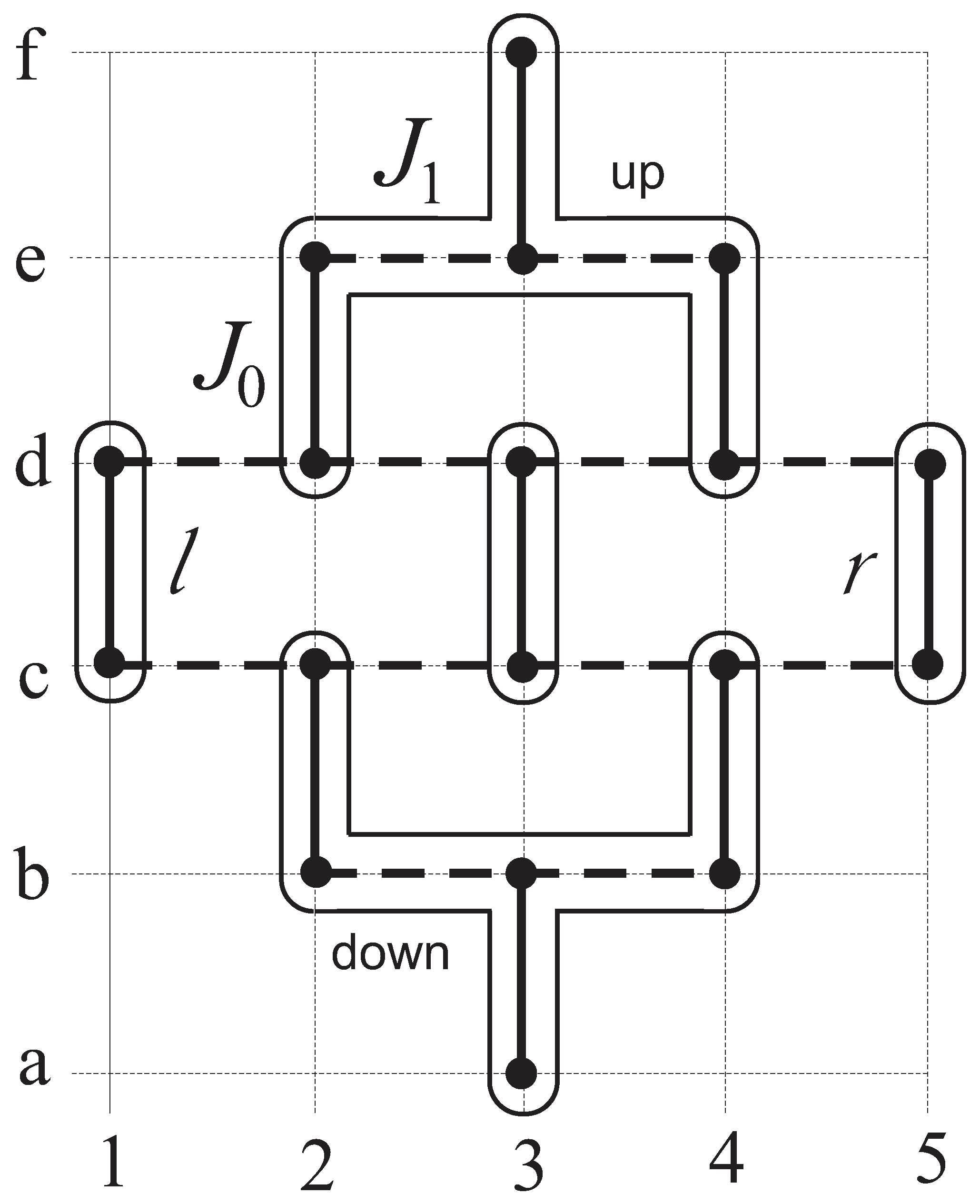
To perform calculations we start with the cluster of minimal size $\sqrt{5}\times \sqrt{5}$. The sequence of clusters involved in the calculations are shown in Figure 1. Within the smallest cluster, the central spin interacts with the nearest environment consisting of the spins $S_{{\alpha }_1},S_{{\beta }_1},S_{{\gamma }_1},S_{{\eta }_1}$. The spin wave functions of the environment with the total spin number $S_u$ and the third component $M_u$ may be written as follows

$$\left|\frac{1}{2}\frac{1}{2}\left(S_{{\alpha }_1{\beta }_1}\right)\frac{1}{2}\frac{1}{2}\left(S_{{\gamma }_1{\eta }_1}\right)S_u{M}_u\right.〉$$

$$=\sum _{m_{{\alpha }_1},m_{{\beta }_1},m_{{\gamma }_1},m_{{\eta }_1}}\sum _{m_{{\alpha }_1{\beta }_1},m_{{\gamma }_1{\eta }_1}}\left[\begin{array}{ccc}1/2& 1/2& S_{{\alpha }_1{\beta }_1}\\ m_{{\alpha }_1}& m_{{\beta }_1}& m_{{\alpha }_1{\beta }_1}\end{array}\right]\left[\begin{array}{ccc}1/2& 1/2& S_{{\gamma }_1{\eta }_1}\\ m_{{\gamma }_1}& m_{{\eta }_1}& m_{{\gamma }_1{\eta }_1}\end{array}\right]\left[\begin{array}{ccc}{S}_{{\alpha }_1{\beta }_1}& S_{{\gamma }_1{\eta }_1}& S_u\\ m_{{\alpha }_1{\beta }_1}& m_{{\gamma }_1{\eta }_1}& M_u\end{array}\right]$$

$$\times \left|1/2m_{{\alpha }_1}\right.〉\left|1/2m_{{\beta }_1}\right.〉\left|1/2m_{{\gamma }_1}\right.〉\left|1/2m_{{\eta }_1}\right.〉.$$

In such a description, all allowed configurations are comprised by a set $\left|00;00\right.〉$, $\left|11;00\right.〉$, $\left|01;1M\right.〉$, $\left|10;1M\right.〉$, $\left|11;1M\right.〉$, $\left|11;2M\right.〉$, where we have dropped the spin $1/2$ arguments for notation convenience. It is easy to see that the functions $\left|S_{{\alpha }_1{\beta }_1}{S}_{{\gamma }_1{\eta }_1};S_u{M}_u\right.〉$ form (in common case) a basis of reducible representation of the group $D_4$ (for details see Appendix C [39])

$$\widehat{g}\left|S_{{\alpha }_1{\beta }_1}{S}_{{\gamma }_1{\eta }_1};S_u{M}_u\right.〉=D_{S_{{\alpha }_1{\beta }_1}^{\prime }{S}_{{\gamma }_1{\eta }_1}^{\prime },S_{{\alpha }_1{\beta }_1}{S}_{{\gamma }_1{\eta }_1}}^{\left(S_u\right)}\left(\widehat{g}\right)\left|S_{{\alpha }_1{\beta }_1}^{\prime }{S}_{{\gamma }_1{\eta }_1}^{\prime };S_u{M}_u\right.〉.$$

The matrices $D_{\kappa ,{\kappa }^{\prime }}^{\left(0\right)}\left(\widehat{g}\right)$ (the upper index denotes the spin $S_u$) with the multiindex $\kappa =\left\{S_{{\alpha }_1{\beta }_1}{S}_{{\gamma }_1{\eta }_1}\right\}$ are readily determined and read

$$D_{\kappa ,{\kappa }^{\prime }}^{\left(0\right)}\left(E\right)=D_{\kappa ,{\kappa }^{\prime }}^{\left(0\right)}\left(C_4^2\right)=D_{\kappa ,{\kappa }^{\prime }}^{\left(0\right)}\left({\sigma }_v^{{}^{\prime }}\right)=D_{\kappa ,{\kappa }^{\prime }}^{\left(0\right)}\left({\sigma }_v^{″}\right)=\left(\begin{array}{cc}1& 0\\ 0& 1\end{array}\right),$$

$$D_{\kappa ,{\kappa }^{\prime }}^{\left(0\right)}\left(C_4\right)=D_{\kappa ,{\kappa }^{\prime }}^{\left(0\right)}\left(C_4^3\right)=D_{\kappa ,{\kappa }^{\prime }}^{\left(0\right)}\left(C_2^x\right)=D_{\kappa ,{\kappa }^{\prime }}^{\left(0\right)}\left(C_4^2\right)=\left(\begin{array}{cc}1/2& -\sqrt{3}/2\\ -\sqrt{3}/2& -1/2\end{array}\right).$$

The functions $\left|00;00\right.〉$, $\left|11;00\right.〉$ form a basis of this two-dimensional representation. Still another representation of $D_4$ can be generated by means of the functions $\left|01;1M\right.〉$, $\left|10;1M\right.〉$ and $\left|11;1M\right.〉$

$$D_{\kappa ,{\kappa }^{\prime }}^{\left(1\right)}\left(E\right)=\left(\begin{array}{ccc}1& 0& 0\\ 0& 1& 0\\ 0& 0& 1\end{array}\right),D_{\kappa ,{\kappa }^{\prime }}^{\left(1\right)}\left(C_4\right)=\left(\begin{array}{ccc}-1/2& -1/2& 1/\sqrt{2}\\ -1/2& -1/2& -1/\sqrt{2}\\ -1/\sqrt{2}& 1/\sqrt{2}& 0\end{array}\right),$$

$$D_{\kappa ,{\kappa }^{\prime }}^{\left(1\right)}\left(C_4^2\right)=\left(\begin{array}{ccc}0& 1& 0\\ 1& 0& 0\\ 0& 0& -1\end{array}\right),D_{\kappa ,{\kappa }^{\prime }}^{\left(1\right)}\left(C_4^3\right)=\left(\begin{array}{ccc}-1/2& -1/2& -1/\sqrt{2}\\ -1/2& -1/2& 1/\sqrt{2}\\ 1/\sqrt{2}& -1/\sqrt{2}& 0\end{array}\right),$$

$$D_{\kappa ,{\kappa }^{\prime }}^{\left(1\right)}\left(C_2^x\right)=\left(\begin{array}{ccc}1/2& 1/2& 1/\sqrt{2}\\ 1/2& 1/2& -1/\sqrt{2}\\ 1/\sqrt{2}& -1/\sqrt{2}& 0\end{array}\right),D_{\kappa ,{\kappa }^{\prime }}^{\left(1\right)}\left(C_2^y\right)=\left(\begin{array}{ccc}1/2& 1/2& -1/\sqrt{2}\\ 1/2& 1/2& 1/\sqrt{2}\\ -1/\sqrt{2}& 1/\sqrt{2}& 0\end{array}\right),$$

$$D_{\kappa ,{\kappa }^{\prime }}^{\left(1\right)}\left({\sigma }_v^{″}\right)=\left(\begin{array}{ccc}-1& 0& 0\\ 0& -1& 0\\ 0& 0& 1\end{array}\right),D_{\kappa ,{\kappa }^{\prime }}^{\left(1\right)}\left({\sigma }_v^{{}^{\prime }}\right)=\left(\begin{array}{ccc}0& -1& 0\\ -1& 0& 0\\ 0& 0& -1\end{array}\right).$$

In a similar way we find the matrices $D_{\kappa ,\kappa }^{\left(2\right)}\left(\widehat{g}\right)$ in the basis $\left|11;2M\right.〉$

$$D_{\kappa ,\kappa }^{\left(2\right)}\left(\widehat{g}\right)=1(\forall \widehat{g}\in D_4).$$

The representations $D^{\left(S\right)}$ are the direct sums of the irreducible representations $D^{\left(0\right)}=D^{\left(0A_1\right)}\oplus D^{\left(0B_2\right)},$ $D^{\left(1\right)}=D^{\left(1B_1\right)}\oplus D^{\left(1E\right)},$ $D^{\left(2\right)}=D^{\left(2A_1\right)}$. The basis functions of these irreducible representations are given by a similarity transformation

$$\left|S_u{M}_u;\Gamma \mu \right.〉=\sum _{S_{{\alpha }_1{\beta }_1},S_{{\gamma }_1{\eta }_1}}{\widehat{T}}_{S_{{\alpha }_1{\beta }_1}{S}_{{\gamma }_1{\eta }_1};\Gamma \mu }^{\left(S_u\right)}\left|S_{{\alpha }_1{\beta }_1}{S}_{{\gamma }_1{\eta }_1};S_u{M}_u\right.〉,$$

(9)

and the matrix ${\widehat{T}}_{S_{{\alpha }_1{\beta }_1}{S}_{{\gamma }_1{\eta }_1};\Gamma \mu }^{\left(S_u\right)}={\widehat{T}}_{S_{{\alpha }_1{\beta }_1}{S}_{{\gamma }_1{\eta }_1}S{{}_u}^{\prime };S_u{\Gamma }_u{\mu }_u}{\delta }_{S_u,S_u^{\prime }}$ found with the aid of the projection-operator technique reads (for details see Appendix D [39])

$$\begin{array}{ccccccc}& \left|00;A_{1}1\right.〉& \left|00;B_{2}1\right.〉& \left|1M;B_{1}1\right.〉& \left|1M;E1\right.〉& \left|1M;E2\right.〉& \left|2M;A_{1}1\right.〉\\ \left|00;00\right.〉\hfill & \frac{\sqrt{3}}{2}& \frac{1}{2}& 0& 0& 0& 0\\ \left|11;00\right.〉\hfill & -\frac{1}{2}& \frac{\sqrt{3}}{2}& 0& 0& 0& 0\\ \left|01;1M\right.〉\hfill & 0& 0& \frac{1}{\sqrt{2}}& \frac{1}{2}& \frac{1}{2}& 0\\ \left|10;1M\right.〉\hfill & 0& 0& \frac{1}{\sqrt{2}}& -\frac{1}{2}& -\frac{1}{2}& 0\\ \left|11;1M\right.〉\hfill & 0& 0& 0& \frac{1}{\sqrt{2}}& -\frac{1}{\sqrt{2}}& 0\\ \left|11;2M\right.〉\hfill & 0& 0& 0& 0& 0& 1\end{array}$$

Given the environment eigenfunctions $\left|S_u{M}_u;{\Gamma }_u{\mu }_u\right.〉$ with the eigenvalues $E_{S_u{\Gamma }_{{}_u}}$, the RMEs of the double irreducible tensor $O^{1A_1}=S_{{\alpha }_1}+S_{{\beta }_1}+S_{{\gamma }_1}+S_{{\eta }_1}$ can be computed straightforwardly using the Wigner-Eckart theorem and the similarity transformation (9)

$${\left[\begin{array}{ccc}\gamma & {\Gamma }^{\prime }& \Gamma \\ \nu & {\mu }^{\prime }& \mu \end{array}\right]}^{*}〈S\Gamma ∥O^{1\gamma }∥S^{\prime }{\Gamma }^{\prime }〉$$

$$=\sum _{S_{12},S_{34}}\sum _{S_{12}^{\prime },S_{34}^{\prime }}{\widehat{T}}_{S_{12}{S}_{34}S;S\Gamma \mu }^{*}{\widehat{T}}_{S_{12}^{\prime }{S}_{34}^{\prime }{S}^{\prime };S^{\prime }{\Gamma }^{\prime }{\mu }^{\prime }}〈S_{12}{S}_{34};S∥O_{\nu }^{1\gamma }∥S_{12}^{\prime }{S}_{34}^{\prime };S^{\prime }〉,$$

(10)

where the indices ${\alpha }_1$, ${\beta }_1$, ${\gamma }_1$, ${\eta }_1$ are correspondingly denoted by the numbers 1-4.

To calculate the RME that comes into the right-hand side of Equation (10) one has to rewrite $O_{q\nu }^{1\gamma }$ through the spin operators and employ their expressions for the RMEs of the spin operators

$$〈S_{12}{S}_{34};S∥S_1∥S_{12}^{\prime }{S}_{34}^{\prime };S^{\prime }〉={\left(-1\right)}^{1+S_{12}+S_{34}+S_{12}^{\prime }+S^{\prime }}{\left[S_{12},S_{12}^{\prime },S,S^{\prime }\right]}^{1/2}$$

$$\times \left\{\begin{array}{ccc}{S}_{12}^{\prime }& 1& S_{12}\\ 1/2& 1/2& 1/2\end{array}\right\}\left\{\begin{array}{ccc}{S}^{\prime }& 1& S\\ S_{12}& S_{34}& S_{12}^{\prime }\end{array}\right\}〈1/2∥S∥1/2〉{\delta }_{S_{34},S_{34}^{\prime }},$$

(11)

$$〈S_{12}{S}_{34};S∥S_2∥S_{12}^{\prime }{S}_{34}^{\prime };S^{\prime }〉={\left(-1\right)}^{1+2S_{12}+S_{34}+S^{\prime }}{\left[S_{12},S_{12}^{\prime },S,S^{\prime }\right]}^{1/2}$$

$$\times \left\{\begin{array}{ccc}{S}_{12}^{\prime }& 1& S_{12}\\ 1/2& 1/2& 1/2\end{array}\right\}\left\{\begin{array}{ccc}{S}^{\prime }& 1& S\\ S_{12}& S_{34}& S_{12}^{\prime }\end{array}\right\}〈1/2∥S∥1/2〉{\delta }_{S_{34},S_{34}^{\prime }},$$

(12)

$$〈S_{12}{S}_{34};S∥S_3∥S_{12}^{\prime }{S}_{34}^{\prime };S^{\prime }〉={\left(-1\right)}^{1+S_{12}+2S_{34}^{\prime }+S}{\left[S_{34},S_{34}^{\prime },S,S^{\prime }\right]}^{1/2}$$

$$\times \left\{\begin{array}{ccc}{S}_{34}^{\prime }& 1& S_{34}\\ 1/2& 1/2& 1/2\end{array}\right\}\left\{\begin{array}{ccc}{S}^{\prime }& 1& S\\ S_{34}& S_{12}& S_{34}^{\prime }\end{array}\right\}〈1/2∥S∥1/2〉{\delta }_{S_{12},S_{12}^{\prime }},$$

(13)

$$〈S_{12}{S}_{34};S∥S_4∥S_{12}^{\prime }{S}_{34}^{\prime };S^{\prime }〉={\left(-1\right)}^{1+S_{12}+S_{34}+S_{34}^{\prime }+S}{\left[S_{34},S_{34}^{\prime },S,S^{\prime }\right]}^{1/2}$$

$$\times \left\{\begin{array}{ccc}{S}_{34}^{\prime }& 1& S_{34}\\ 1/2& 1/2& 1/2\end{array}\right\}\left\{\begin{array}{ccc}{S}^{\prime }& 1& S\\ S_{34}& S_{12}& S_{34}^{\prime }\end{array}\right\}〈1/2∥S∥1/2〉{\delta }_{S_{12},S_{12}^{\prime }}.$$

(14)

Since the operator $O^{1A_1}$ coincides with that of the environment total spin ${\widehat{S}}_u$, it turns out that the matrix elements $〈S_u{\Gamma }_u\left|O^{1A_1}\right|S_u^{\prime }{\Gamma }_u^{\prime }〉$ are diagonal

$$〈S_u{\Gamma }_u\left|O^{1A_1}\right|S_u^{\prime }{\Gamma }_u^{\prime }〉=\sqrt{S_u(S_u+1)(2S_u+1)}{\delta }_{S_u,S_u^{\prime }}{\delta }_{{\Gamma }_u,{\Gamma }_u^{\prime }}.$$

As a consequence, one may check that this property holds for the Hamiltonian of the total cluster

$$〈S_u{\Gamma }_u;\frac{1}{2};SM{\Gamma }_u{\mu }_u\left|\widehat{H}\right|S_u^{\prime }{\Gamma }_u^{\prime };\frac{1}{2};S^{\prime }{M}^{\prime }{\Gamma }_u^{\prime }{\mu }_u^{\prime }〉$$

$$=J{(-1)}^{S_u^{\prime }+S+1/2}\left\{\begin{array}{ccc}{S}_u& 1/2& S\\ 1/2& S_u^{\prime }& 1\end{array}\right\}\sqrt{\frac{3}{2}{S}_u(S_u+1)(2S_u+1)}{\delta }_{S,S^{\prime }}{\delta }_{M,M^{\prime }}{\delta }_{{\Gamma }_u,{\Gamma }_u^{\prime }}{\delta }_{{\mu }_u,{\mu }_u^{\prime }}{\delta }_{S_u,S_u^{\prime }}$$

A direct calculation shows that the ground state belongs to the Hilbert space sector with $S=3/2$ and $\Gamma =A_1$. Hence, only the environment state with $S\Gamma =1A_1$ is needed to find the ground state energy (see

Table 1. Energies $E_{S\Gamma }$ and ${ϵ}_{S\Gamma }$.

$S\Gamma$	$\frac{1}{2}{A}_1$	$\frac{1}{2}{B}_1$	$\frac{1}{2}{B}_2$	$\frac{1}{2}E$	$\frac{3}{2}{A}_1$	$\frac{3}{2}{B}_1$	$\frac{3}{2}E$	$\frac{5}{2}{A}_1$
$E_{S\Gamma }$	0	−J	0	−J	$-\frac{3}{2}J$	$\frac{1}{2}J$	$\frac{1}{2}J$	J
${ϵ}_{S\Gamma }$	0	− $\frac{1}{4}J$	0	$-\frac{1}{4}J$	$-\frac{3}{8}J$	$\frac{1}{8}J$	$\frac{1}{8}J$	$\frac{1}{4}J$

).

Let us now consider the next step, an expansion of the current environment block due to the next coordination sphere of radius $\sqrt{2}$. After an addition of four spins $S_a,S_b,S_c,S_d$, the cluster becomes a square of size $3\times 3$ with the bipartite environment of the central site (Figure 1). The basis associated with the added part is

$$\left|\frac{1}{2}\frac{1}{2}\left(S_{ab}\right)\frac{1}{2}\frac{1}{2}\left(S_{cd}\right)S_I{M}_I\right.〉$$

$$=\sum _{m_a,m_b,m_c,m_d}\sum _{m_{ab},m_{cd}}\left[\begin{array}{ccc}1/2& 1/2& S_{ab}\\ m_a& m_b& m_{ab}\end{array}\right]\left[\begin{array}{ccc}1/2& 1/2& S_{cd}\\ m_c& m_d& m_{cd}\end{array}\right]\left[\begin{array}{ccc}{S}_{ab}& S_{cd}& S_I\\ m_{ab}& m_{cd}& M_I\end{array}\right]$$

$$\times \left|1/2m_a\right.〉\left|1/2m_b\right.〉\left|1/2m_c\right.〉\left|1/2m_d\right.〉.$$

(15)

Repeating the basic steps in the approach we obtain the symmetry adapted basis $\left|S_I{M}_I;{\Gamma }_I{\mu }_I\right.〉$. The matrix of corresponding similarity transformation has the form

$$\begin{array}{ccccccc}& \left|00;A_{1}1\right.〉& \left|00;B_{1}1\right.〉& \left|1M;B_{2}1\right.〉& \left|1M;E1\right.〉& \left|1M;E2\right.〉& \left|2M;A_{1}1\right.〉\\ \left|00;00\right.〉\hfill & \frac{\sqrt{3}}{2}& \frac{1}{2}& 0& 0& 0& 0\\ \left|11;00\right.〉\hfill & -\frac{1}{2}& \frac{\sqrt{3}}{2}& 0& 0& 0& 0\\ \left|01;1M\right.〉\hfill & 0& 0& \frac{1}{\sqrt{2}}& 0& \frac{1}{\sqrt{2}}& 0\\ \left|10;1M\right.〉\hfill & 0& 0& \frac{1}{\sqrt{2}}& 0& -\frac{1}{\sqrt{2}}& 0\\ \left|11;1M\right.〉\hfill & 0& 0& 0& 1& 0& 0\\ \left|11;2M\right.〉\hfill & 0& 0& 0& 0& 0& 1\end{array}$$

The environment Hamiltonian includes only interactions between the first and second coordination spheres

$${\widehat{H}}_u=J\left[{\overrightarrow{S}}_{{\alpha }_1}\left({\overrightarrow{S}}_d+{\overrightarrow{S}}_a\right)+{\overrightarrow{S}}_{{\beta }_1}\left({\overrightarrow{S}}_a+{\overrightarrow{S}}_b\right)+{\overrightarrow{S}}_{{\gamma }_1}\left({\overrightarrow{S}}_b+{\overrightarrow{S}}_c\right)+{\overrightarrow{S}}_{{\eta }_1}\left({\overrightarrow{S}}_c+{\overrightarrow{S}}_d\right)\right].$$

(16)

We now introduce the cluster irreducible tensors $W_{q\mu }^{1\Gamma }$ and $U_{q\mu }^{1\Gamma }$ transforming according to representations $\Gamma \mu$ of the point symmetry group $D_4$ (for details see Appendix D [39])

$$U_{q1}^{1A_1}=\frac{1}{\sqrt{2}}\left(S_{aq}+S_{bq}+S_{cq}+S_{dq}\right),U_{q1}^{1B_2}=\frac{1}{\sqrt{2}}\left(S_{aq}-S_{bq}+S_{cq}-S_{dq}\right),$$

$$U_{q1}^{1E}=\frac{1}{\sqrt{2}}\left(S_{aq}+S_{bq}-S_{cq}-S_{dq}\right),U_{q2}^{1E}=\frac{1}{\sqrt{2}}\left(S_{aq}-S_{bq}-S_{cq}+S_{dq}\right),$$

$$W_{q1}^{1A_1}=\frac{1}{\sqrt{2}}\left(S_{{\alpha }_{1}q}+S_{{\beta }_{1}q}+S_{{\gamma }_{1}q}+S_{{\eta }_{1}q}\right),W_{q1}^{1B_1}=\frac{1}{\sqrt{2}}\left(S_{{\alpha }_{1}q}-S_{{\beta }_{1}q}+S_{{\gamma }_{1}q}-S_{{\eta }_{1}q}\right),$$

$$W_{q1}^{1E}=\left(S_{{\alpha }_{1}q}-S_{{\gamma }_{1}q}\right),W_{q2}^{1E}=\left(S_{{\eta }_{1}q}-S_{{\beta }_{1}q}\right)$$

(17)

and then rewrite Equation (16) as

$$H_u=J\sum _{\gamma \nu }\sum _q{(-1)}^q\left[\begin{array}{ccc}\gamma & \gamma & A_1\\ \nu & \nu & 1\end{array}\right]U_{q\mu }^{1\gamma }{W}_{-q\mu }^{1\gamma }=J\sum _{\gamma }{\left[U^{1\gamma }\times W^{1\gamma }\right]}_{01}^{0A_1}.$$

(18)

The RMEs of the irreducible operators that appear in Equation (8) can be obtained exactly from the result (10)

$$〈S_I{\Gamma }_I∥U^{1A_1}∥S_I^{\prime }{\Gamma }_I^{\prime }〉=\frac{1}{\sqrt{2}}〈S_I∥S∥S_I〉{\delta }_{S_I,S_I^{\prime }}{\delta }_{{\Gamma }_I,{\Gamma }_I^{\prime }},$$

(19)

$$〈S_{II}{\Gamma }_{II}∥W^{1A_1}∥S_{II}^{\prime }{\Gamma }_{II}^{\prime }〉=\frac{1}{\sqrt{2}}〈S_{II}∥S∥S_{II}〉{\delta }_{S_{II},S_{II}^{\prime }}{\delta }_{{\Gamma }_{II},{\Gamma }_{II}^{\prime }},$$

$$〈S_I{\Gamma }_I∥U^{1E}∥S_I^{\prime }{\Gamma }_I^{\prime }〉=\left[\begin{array}{cccccc}& 0A_1& 0B_1& 1B_2& 1E& 2A_1\\ 0A_1& 0& 0& 0& \sqrt{2}& 0\\ 0B_1& 0& 0& 0& -\sqrt{6}& 0\\ 1B_2& 0& 0& 0& -\sqrt{6}& 0\\ 1E& -1& \sqrt{3}& -\sqrt{3}& 0& -\sqrt{5}\\ 2A_1& 0& 0& 0& \sqrt{10}& 0\end{array}\right],$$

$$〈S_{II}{\Gamma }_{II}∥W^{1E}∥S_{II}^{\prime }{\Gamma }_{II}^{\prime }〉=\left[\begin{array}{cccccc}& 0A_1& 0B_2& 1B_1& 1E& 2A_1\\ 0A_1& 0& 0& 0& \sqrt{2}& 0\\ 0B_2& 0& 0& 0& \sqrt{6}& 0\\ 1B_1& 0& 0& 0& -\sqrt{6}& 0\\ 1E& -1& -\sqrt{3}& -\sqrt{3}& 0& -\sqrt{5}\\ 2A_1& 0& 0& 0& \sqrt{10}& 0\end{array}\right].$$

To compute matrix elements of the Hamiltonian $H_u$ we construct the basis

$$\left|i_I{S}_I{\Gamma }_I{i}_{II}{S}_{II}{\Gamma }_{II};S_u{M}_u{\Gamma }_u{\mu }_u\right.〉$$

$$=\sum _{m_I,m_{II}}\sum _{{\mu }_I,{\mu }_{II}}\left[\begin{array}{ccc}{S}_I& S_{II}& S_u\\ m_I& m_{II}& M_u\end{array}\right]\left[\begin{array}{ccc}{\Gamma }_I& {\Gamma }_{II}& {\Gamma }_u\\ {\mu }_I& {\mu }_{II}& {\mu }_u\end{array}\right]\left|i_I{S}_I{m}_I{\Gamma }_I{\mu }_I\right.〉\left|i_{II}{S}_{II}{m}_{II}{\Gamma }_{II}{\mu }_{II}\right.〉$$

(20)

formed from the eigenstates $\left|i_I{S}_I{m}_I{\Gamma }_I{\mu }_I\right.〉$ and $\left|i_{II}{S}_{II}{m}_{II}{\Gamma }_{II}{\mu }_{II}\right.〉$ of the “new” and “old” added parts, correspondingly. The expression for the matrix $H_u$ is similar to Equation (8) with $E_{i_I{S}_I{\Gamma }_I}=E_{i_{II}{S}_{II}{\Gamma }_{II}}=0$. Applying exact diagonalization to the Hamiltonian $H_u$ one can then find the eigenfunctions

$$\left|i_u{S}_u{\Gamma }_u{\mu }_u\right.〉=\sum {\alpha }_{i_I{S}_I{\Gamma }_I;i_{II}{S}_{II}{\Gamma }_{II}}^{i_u{S}_u{\Gamma }_u}\left|i_I{S}_I{\Gamma }_I{i}_{II}{S}_{II}{\Gamma }_{II};S_u{M}_u{\Gamma }_u{\mu }_u\right.〉$$

and the energy spectrum $E_{i_u{S}_u{\Gamma }_u}$ of the environment. By using the recursion relation (for details see Appendix B [39])

$$〈i_u{S}_u{\Gamma }_u∥O^{1A_1}∥i_u^{\prime }{S}_u^{\prime }{\Gamma }_u^{\prime }〉={\delta }_{{\Gamma }_u,{\Gamma }_u^{\prime }}\sum _{i_I,S_I,\Gamma }\sum _{i_{II}^{\prime },S_{II}^{\prime },{\Gamma }_{II}^{\prime }}\sum _{i_{II},S_{II},{\Gamma }_{II}}{\alpha }_{i_I{S}_I{\Gamma }_I;i_{II}{S}_{II}{\Gamma }_{II}}^{i_u{S}_u{\Gamma }_u}{\alpha }_{i_I{S}_I{\Gamma }_I;i_{II}^{\prime }{S}_{II}^{\prime }{\Gamma }_{II}^{\prime }}^{i_u^{\prime }{S}_u^{\prime }{\Gamma }_u^{\prime }}$$

$$\times {\left(-1\right)}^{1+S_I+S_{II}^{\prime }+S_u}{\left[S_u,S_u^{\prime }\right]}^{1/2}\left\{\begin{array}{ccc}{S}_u& 1& S_u^{\prime }\\ S_{II}^{\prime }& S_I& S_{II}\end{array}\right\}〈i_{II}{S}_{II}{\Gamma }_{II}∥O^{1A_1}∥i_{II}^{\prime }{S}_{II}^{\prime }{\Gamma }_{II}^{\prime }〉$$

(21)

one finds the RMEs in the environment basis $\left|i_u{S}_u{A}_1\right.〉$ that come into the matrix of the total cluster (3).

The formulas (3,4,5) allow us to obtain any of possible 54 square cluster states. Our calculation shows that the ground state belongs to the Hilbert space sector with $S=1/2$ and $\Gamma =A_1$. Hence, only the environment states with $S\Gamma =0A_1$, $1A_1$ are needed for the evaluation of the ground state energy. Below we summarize the results obtained for this particular case.

Using Equation (8) and the explicit expressions for the nonzero sums of Clebsch-Gordan coefficients of the point group $D_4$ (see Appendix A [39])

$$F(A_1{A}_1{A}_1;A_1,A_1,A_1)=F(EE{A}_1;A_1{A}_{1}E)=1,$$

$$F(EE{A}_1;EE{A}_1)=1,F(A_1{A}_1{A}_1;EEE)=1/2,$$

we obtain

$${\widehat{H_u}}^{\left(0A_1\right)}=\left[\begin{array}{ccc}0& -\frac{1}{\sqrt{3}}J& 0\\ -\frac{1}{\sqrt{3}}J& -J& -\sqrt{\frac{5}{3}J}\\ 0& -\sqrt{\frac{5}{3}J}& -3J\end{array}\right]$$

in the basis of the states $\left|0A_{1}0A_1;00A_1\right.〉,\left|1E1E;00A_1\right.〉,\left|2A_{1}2A_1;00A_1\right.〉$. The diagonalization of ${\widehat{H_u}}^{\left(0A_1\right)}$ yields three states of the $0A_1$ symmetry (see

Table 2. Environment states of symmetry $0A_1$.

$i_u$	${\alpha }_{0A_{1}0A_1}^{i_{u}0A_1}$	${\alpha }_{1E1E}^{i_{u}0A_1}$	${\alpha }_{2A_{1}2A_1}^{i_{u}0A_1}$	$E_{i_{u}0A_1}$
1	0.071	0.449	0.890	−3.651 J
2	0.569	0.715	−0.406	−0.726 J
3	−0.819	0.535	−0.205	0.377 J

)

As for the $\widehat{H_u}$-operator with $S_u=1$, we have the following matrix representation, with the same considerations as for the ${\widehat{H_u}}^{\left(0A_1\right)}$-operator,

$${\widehat{H_u}}^{\left(1A_1\right)}=\left[\begin{array}{cccc}0& 0& J& 0\\ 0& 0& J& 0\\ J& J& -\frac{1}{2}J& -\frac{\sqrt{5}}{2}J\\ 0& 0& -\frac{\sqrt{5}}{2}J& -\frac{5}{2}J\end{array}\right]$$

in the basis $\left|0B_{1}1B_1;1M{A}_1\right.〉,\left|1B_{2}0B_2;1M{A}_1\right.〉,\left|1E1E;1M{A}_1\right.〉,\left|2A_{1}2A_1;1M{A}_1\right.〉$. The states of $1A_1$ symmetry are listed in

Table 3. Environment states of symmetry $1A_1$.

$i_u$	${\alpha }_{0A_{3}1A_3}^{i_{u}1A_1}$	${\alpha }_{1A_{4}0A_4}^{i_{u}1A_1}$	${\alpha }_{1E1E}^{i_{u}1A_1}$	${\alpha }_{2A_{1}2A_1}^{i_{u}1A_1}$	$E_{i_{u}1A_1}$
1	0.153	0.153	−0.478	−0.851	−3.128 J
2	−0.470	−0.470	0.566	−0.487	−1.202 J
3	−0.505	−0.505	−0.672	0.196	1.330 J
4	−0.707	0.707	0	0	0

.

By using the recursion relation (21) with the starting value (2), one finds the RMEs in the environment basis $\left|i_u{S}_u{A}_1\right.〉$. Plugging them into Equation (3) we get the target states $\left|i\frac{1}{2}M{A}_1\right.〉$ [see Equation (5)] of the cluster and their energies $E_{i\frac{1}{2}{A}_1}$ ($i=1..7$). The number of states involved in determining the cluster ground state equals 7 (see

Table 4. Data on the ground state of the cluster $3\times 3$.

${\beta }_{10A_1}^g$	${\beta }_{20A_1}^g$	${\beta }_{30A_1}^g$	${\beta }_{11A_1}^g$	${\beta }_{21A_1}^g$	${\beta }_{31A_1}^g$	${\beta }_{41A_1}^g$	$E_g$
−0.712	0.044	0.010	−0.695	0.0048	−0.090	0.011	−4.749

).

Now we list the results for observables. The energy per bond found with the help of Equation (4) is ${\epsilon }_g=-0.3442J$. This result may be compared to those results of QMC [23] ${\epsilon }_g=-0.3347J$, and DMRG ${\epsilon }_g=-0.32679J$ for lattice of size $20\times 20$ and for number of DMRG states 150 [22]. (Extrapolation of the DMRG results in the infinite-lattice limit yields ${\epsilon }_g=-0.3321J$). The best available dressed cluster method (DCM) [42], coupled cluster method (CCM) [43] and real-space renormalization group with effective interactions (RSRG-EI) [44] results are $-0.33486J,$ $-0.33308J,$ and $-0.33409J$, respectively. Using (6) we get the ground-state expectation value of the z component of the central spin ${〈S_0^z〉}_0=0.173$ and the staggered magnetization $M=\sqrt{3{〈S_0^z〉}_0^2}=0.299$. For comparison, the extrapolated QMC result for the lattice magnetization $M=0.3070$. We also provide an estimate of the spin-spin correlation functions (7)

$$〈S_0^z{S}_{r=1}^z〉=-0.115,〈S_0^z{S}_{r=\sqrt{2}}^z〉=0.073.$$

These estimates should be compared with the known results -0.1116 and 0.0637, correspondingly [45].

We have made a preliminary calculations by using the small cluster $3\times 3$ and one can see that an accuracy of the results is still insufficient. At further step, the procedure is repeated and the environment block grows by adding the coordination sphere of radius 2. When the new spins ${\overrightarrow{S}}_{{\alpha }_2}$, ${\overrightarrow{S}}_{{\beta }_2}$, ${\overrightarrow{S}}_{{\gamma }_2}$, ${\overrightarrow{S}}_{{\eta }_2}$ of the sphere are added, the cluster transforms into the rhombus of size $\sqrt{13}\times \sqrt{13}$. The cluster has the non-bipartite environment, hence, it is instructive to study this case to examine the effect of non-biparticity.

The Hamiltonian of the new environment decomposes as

$${\widehat{H}}_u=H_u\left(0\right)+J\left({\overrightarrow{S}}_{{\alpha }_1}{\overrightarrow{S}}_{{\alpha }_2}+{\overrightarrow{S}}_{{\beta }_1}{\overrightarrow{S}}_{{\beta }_2}+{\overrightarrow{S}}_{{\gamma }_1}{\overrightarrow{S}}_{{\gamma }_2}+{\overrightarrow{S}}_{{\eta }_1}{\overrightarrow{S}}_{{\eta }_2}\right).$$

(22)

$H_u\left(0\right)$ contains all interactions within the “old” environment, and the second term describes all couplings between this part and the added sites.

The irreducible tensors built from the added spins are the same as those of the first coordination sphere (17)

$$W_{q1}^{1A_1}=\frac{1}{\sqrt{2}}\left(S_{{\alpha }_{2}q}+S_{{\beta }_{2}q}+S_{{\gamma }_{2}q}+S_{{\eta }_{2}q}\right),W_{q1}^{1B_1}=\frac{1}{\sqrt{2}}\left(S_{{\alpha }_{2}q}-S_{{\beta }_{2}q}+S_{{\gamma }_{2}q}-S_{{\eta }_{2}q}\right),$$

$$W_{q1}^{1E}=\left(S_{{\alpha }_{2}q}-S_{{\gamma }_{2}q}\right),W_{q2}^{1E}=\left(S_{{\eta }_{2}q}-S_{{\beta }_{2}q}\right).$$

(23)

One can then cast the Hamiltonian (22) in a more amenable form

$${\widehat{H}}_u={\widehat{H}}_u\left(0\right)+\frac{1}{2}J{\left[U^{1A_1}\times W^{1A_1}\right]}_{01}^{0A_1}+\frac{1}{2}J{\left[U^{1B_1}\times W^{1B_1}\right]}_{01}^{0A_1}+\frac{1}{\sqrt{2}}J{\left[U^{1E}\times W^{1E}\right]}_{01}^{0A_1},$$

where $U^{1\gamma }$ are given by

$$U_{q1}^{1A_1}=\frac{1}{\sqrt{2}}\left(S_{{\alpha }_{1}q}+S_{{\beta }_{1}q}+S_{{\gamma }_{1}q}+S_{{\eta }_{1}q}\right),U_{q1}^{1B_1}=\frac{1}{\sqrt{2}}\left(S_{{\alpha }_{1}q}-S_{{\beta }_{1}q}+S_{{\gamma }_{1}q}-S_{{\eta }_{1}q}\right),$$

$$U_{q1}^{1E}=\left(S_{{\alpha }_{1}q}-S_{{\gamma }_{1}q}\right),U_{q2}^{1E}=\left(S_{{\eta }_{1}q}-S_{{\beta }_{1}q}\right).$$

(24)

The matrices formed from the RMEs of $W^{1\gamma }$ tensor coincide with (2). To find those of $U^{1\gamma }$ tensor we use Equation (B.5) from Ref. [39]. The expressions mentioned (19) are used to initialize the calculations.

From direct calculations one can show that the quantum numbers $S=5/2$ and $\Gamma =A_1$ are attached to the ground state of the rhombus. This state is formed from 41 environment states with the symmetry $S{\Gamma }_u=2A_1$ and 22 states of symmetry $S{\Gamma }_u=3A_1$. Numerical diagonalization gives the cluster ground state energy $E_g\left(\frac{5}{2}{A}_1\right)=-5.779J$ that yields the ground-state energy per bond ${\epsilon }_g=-0.30925J$ in the thermodynamic limit. If we compare this result with that of QMC, we see that the agreement becomes worse. Nevertheless, the conclusions made for the square cluster $3\times 3$ hold: (i) both the ground state of the environment and that of the total cluster have the lattice point symmetry $A_1$. (ii) The largest weight (is of the order $0.993$) into the sum of diagonal elements in the density matrix comes from three lowest-lying $2A_1$ states and one state of symmetry $3A_1$, whereas the total number of states is 63.

Monitoring energies per bond ${\epsilon }_{iS\Gamma }$ for the total cluster spectrum $E_{iS\Gamma }$, we found that the minimal value ${\epsilon }_{min}\approx -0.3229J$ is reached for the lowest state of symmetry $\frac{3}{2}{A}_1$, however, $E\left(\frac{3}{2}{A}_1\right)>E_g=E\left(\frac{5}{2}{A}_1\right)$. A similar situation, when a minimal energy per bond belongs to a higher lying state, has been early observed in DMRG study of antiferromagnetic chains [19]. Despite the number of sites in the cluster $\sqrt{13}\times \sqrt{13}$ is greater than that of in the cluster $3\times 3$, we see that the result for ${\epsilon }_{min}$ deteriorates compared to the QMC value $-0.3347J$. Close inspection allows us to suggest that this is because we are working on the cluster with a non-bipartite environment.

To proceed with increasing cluster size and satisfy the biparticity requirement we should take the square cluster $5\times 5$ in the next step. For the 24-site environment of the cluster, an exact-diagonalization calculation of the total spectrum is not possible at present and so, to move on to the next-larger system, we have to elaborate a procedure for determining the states giving the best approximation to true environment states. To solve the problem and implement the condition of bipartite environment we take a system in the form of “decorated cross” obtained from the former cluster $\sqrt{13}\times \sqrt{13}$ by adding four spins ${\overrightarrow{S}}_{{\alpha }_3}$, ${\overrightarrow{S}}_{{\beta }_3}$, ${\overrightarrow{S}}_{{\gamma }_3}$, ${\overrightarrow{S}}_{{\eta }_3}$ (Figure 1). The form makes equal a number of sites in both sublattices, though it incorporates 8 sites that are being attached to the cluster by single lattice bonds. At the same time, exact diagonalization of the cluster$\sqrt{17}\times \sqrt{17}$ is allowed, hence we compare the exact diagonalization results with those obtained from a symmetry based truncation procedure and analyze a truncation error on a number of states kept. Since the cluster increasing is similar to that used in the previous step, we present only the results of calculations. The ground state of the extended cluster environment has the symmetry $0A_1$. The total number of states with the same symmetry is 194. Together with 439 $1A_1$-states of the environment they form a ground state of the total cluster labeled by the symmetry numbers $\frac{1}{2}{A}_1$. Results for the ground state energy per bond $\epsilon =-0.3304$, the staggered magnetization $m=0.305$ and the spin-spin correlation functions $〈S_0^z{S}_{r=1}^z〉=-0.1101$, $〈S_0^z{S}_{r=\sqrt{2}}^z〉=0.0615$ agree well with the mentioned ED and QMC results and are much better than those obtained for the square cluster $3\times 3$. A deviation from the ED result is found for $〈S_0^z{S}_{r=2}^z〉=0.0169$. This discrepancy arises from finite size effects and an imperfect topology of the cluster.

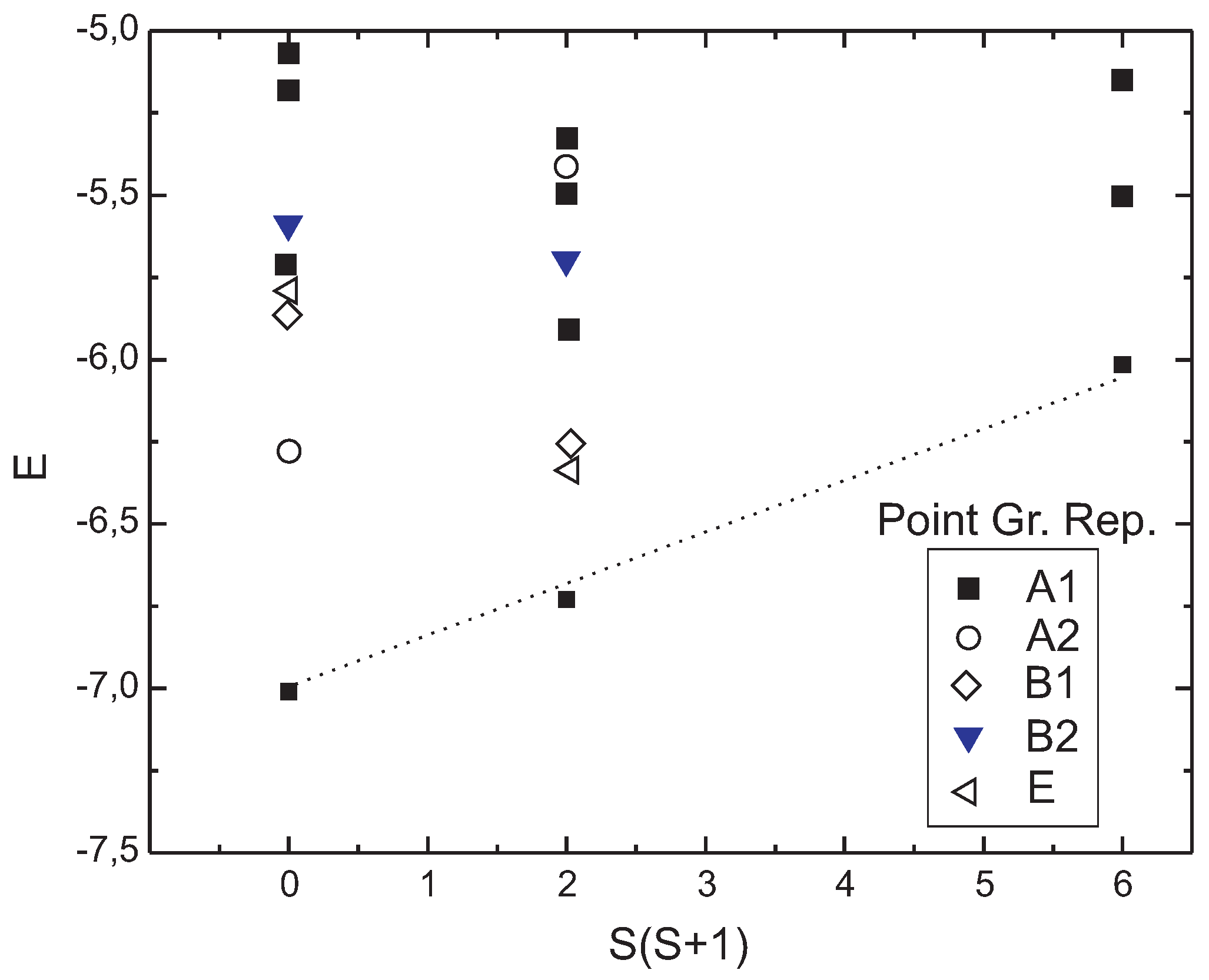
We now describe the low-energy spectrum of the environment. As the dynamics of Néel order parameter is the one of a free rotator, the low-energy levels scale as $E\left(S\right)\sim S(S+1)/N$, where the inertia of that rotator is proportional to the number of sites [46,47]. The environment lowest-energy levels (tower of states) belonging to different irreducible representations of the lattice point group are shown in Figure 2 for different S sectors. The $SU\left(2\right)$ breaking due to long-range Néel order appears as a set of $A_1$-states, lying off from other levels, with an energy scaling as $E\left(S\right)\sim S(S+1)$.

In the remainder of this section we describe a version of the truncation procedure. The main idea will be illustrated on an example of the ground states properties. An inspection of results for the current and previous clusters reveals that one have to take the lowest-lying environment eigenstates both in the $0A_1$ and $1A_1$ sectors. 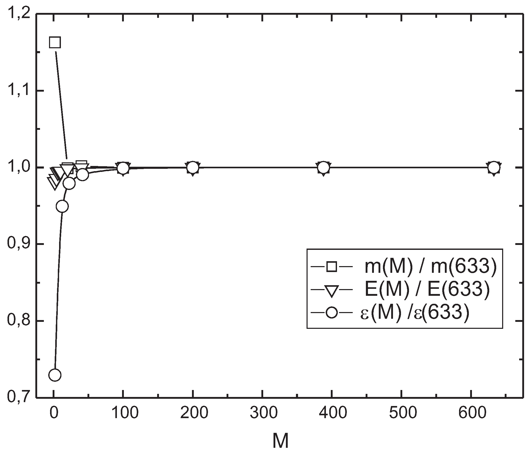As for the number of kept states it seems to be most simple to take M states equally from the both subspaces, albeit the choice may not be optimal. To prove that this concept works we recalculate the observables found above on various number of envronment states kept (see

Table 5. Convergence of the ground state properties vs number of environment states kept.

M(0A1)	M(1A1)	E0/J	$\epsilon /J$	m	$〈S_0^z{S}^z\left(1\right)〉$	$〈S_0^z{S}^z\left(\sqrt{2}\right)〉$
1	1	−7.9010	−0.2410	0.354897	−0.080333	0.065647
5	5	−8.1018	−0.3136	0.304148	−0.104533	0.071420
10	10	−8.1282	−0.3238	0.304928	−0.107933	0.073201
20	20	−8.1378	−0.3279	0.305707	−0.109300	0.073872
50	50	−8.1425	−0.3301	0.305101	−0.110033	0.074247
100	100	−8.1429	−0.3303	0.305187	−0.110100	0.074289
194	194	−8.1430	−0.3304	0.305187	−0.110133	0.074300

). As can be seen from Figure 3 the convergence of the results is exponentially fast in M. Merely keeping 100 basis states may be as efficient as keeping of all 633 environment states intact. We regard the resulting better than 0.01% agreement for $\epsilon$ and $m$ as support for the efficiency of our truncation procedure.

3. Magnetocaloric Effect in Ferrimagnetic Chains

The magnetocaloric effect, i.e., a temperature change induced by an adiabatic change of an external magnetic field was discovered in iron by Warburg [48]. Adiabatic demagnetization of paramagnetic salts was the first method to reach temperatures below 1 K.

Recently, MCE in quantum spin systems attracts a lot of attention. The interest is mainly motivated by universal behavior of quantum phase transitions induced by an applied magnetic field [49,50]. Another reason is that the magnetocaloric effect is enhanced by geometric frustration [51,52]. An unusual MCE is also predicted for non-frustrated quantum ferrimagnetic chains [53].

The magnetization process of the $(S,s)$ ferrimagnetic alternating spin chains is of interest because of possible quantization phenomena detected as a plateau in the magnetization curve. According to Lieb-Schultz-Mattis theorem [54,55], a necessary condition for the plateau is

$$\tilde{S}-m=\mathrm{integer},$$

where $\tilde{S}$ and m are the sum of spins over all sites and the magnetization in the unit period, respectively. For the ferrimagnetic spin chains this means that there is the magnetization plateau $m=S-s$ in the ground state and higher plateaux with $m=S-s+1$, $S-s+2,$ …, $S+s$. It was argued that the ground-state plateau has a quantum origin and it is convenient to introduce the composite spin picture to present the quantum mechanism of the plateau magnetization on the base of Affleck-Kennedy-Lieb-Tasaki valence-bond-solid (VBS) states as has been suggested for Haldane spin chains [56]. As applied to the spin $(S,s)$ ferrimagnet this means that the system behaves like combination of spin-$2s$ antiferromagnet and spin ($S-s$) ferromagnet [57]. Therefore, one may expect a crossover in a magnetocaloric behavior of the $(S,s)$ ferrimagnetic spin chains at low temperatures. Indeed, a magnetic field tuning results in a gap opening for the ferromagnetic excitations, related with the spin ($S-s$) ferromagnetic constituent, in a small-field regime that will be accompanied by an increasing of temperature in an adiabatic magnetization process. Larger fields cause a breaking of the ground VBS state, related with the spin-$2s$ antiferromagnetic constituent, due to condensation of the triplet excitations. It is expected that in the vicinity of the transition an accumulation of entropy will result in an enhanced MCE as found for a class of geometrically frustrated antiferromagnets [51].

Below, we consider the enhanced MCE in the example of the $(5/2,1)$ ferrimagnetic model considered previously in the study of molecule-based heterospin magnets [Mn(hfac)${}_2$BNO${}_R$] (R=H, F, Cl, Br) [58,59]. Our goal is to calculate the entropy $\mathcal{S}$ at the temperature T and the magnetic field H invoking the formalism of $SU\left(2\right)$ group.

The Hamiltonian of the ferrimagnetic ($S,s$) chain reads

$$H=J\sum _{j=1}^N\left({\overrightarrow{S}}_j·{\overrightarrow{s}}_j+{\overrightarrow{s}}_j·{\overrightarrow{S}}_{j+1}\right)$$

(25)

and describes two kinds of spins $S=5/2$ and $s=1$ alternating on a chain with antiferromagnetic exchange coupling $J>0$ between nearest neighbors.

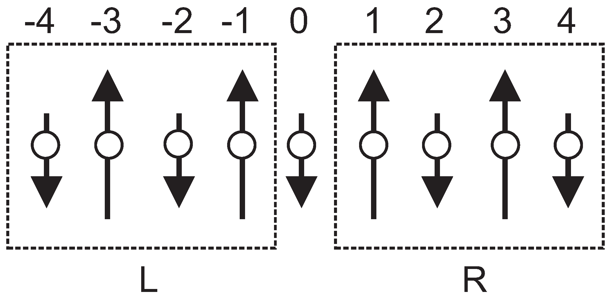
Let us consider a finite-size cluster with $2N+1$ sites as the superblock formed by a left block $B_L$, a central site • and another block $B_R$ (Figure 4). The cluster Hamiltonian

$$H=H_L+H_R+H_{int},$$

(26)

is composed of the terms $H_L\left(H_R\right)$ including all couplings within the left (right) block. The rest term $H_{int}$ describes interaction of the central spin with the nearest neighbors

$$H_{int}=J{\overrightarrow{S}}_0\left({\overrightarrow{S}}_1+{\overrightarrow{S}}_{-1}\right).$$

A Hilbert space of the superblock $B_L•B_R$ can be written as follows. Form eigenvectors the “environment” $B_L\otimes B_R$ of the central site

$$\left|i_l{S}_l{i}_r{S}_r;S_u{M}_u\right.〉=\sum _{m_l,m_r}\left[\begin{array}{ccc}{S}_l& S_r& S_u\\ m_l& m_r& M_u\end{array}\right]\left|i_l{S}_l{m}_l\right.〉\left|i_r{S}_r{m}_r\right.〉$$

(27)

classified with the total spin angular momentum $S_u$ and the corresponding third component $M_u$. The states of the left and right blocks are given by the set $\left|i_l{S}_l{m}_l\right.〉$ and $\left|i_r{S}_r{m}_r\right.〉$, respectively, with the total angular momentum S and the third component m, where the index i labels other possible quantum numbers. The basis functions of the full cluster are obtained by the addition rule of spin angular momentum

$$\left|i_l{S}_l{i}_r{S}_r,S_u{S}_0;SM\right.〉=\sum _{M_u,m_0}\left[\begin{array}{ccc}{S}_u& S_0& S\\ M_u& m_0& M\end{array}\right]\left|i_l{S}_l{i}_r{S}_r;S_u{M}_u\right.〉\left|S_0{m}_0\right.〉,$$

(28)

where $\left|S_0{m}_0\right.〉$ is the wave function of the central spin.

The calculation of matrix elements for the Hamiltonian (26) with the help of the Wigner-Eckart’s theorem [41] yields

$$〈i_l{S}_l{i}_r{S}_r,S_u{S}_0;SM\left|H\right|i_l^{\prime }{S}_l^{\prime }{i}_r^{\prime }{S}_r^{\prime },S_u^{\prime }{S}_0;S^{\prime }{M}^{\prime }〉=\left(E_{i_l{S}_l}+E_{i_r{S}_r}\right){\delta }_{i_l,i_l^{\prime }}{\delta }_{S_l,S_l^{\prime }}{\delta }_{i_r,i_r^{\prime }}{\delta }_{S_r,S_r^{\prime }}{\delta }_{S_u{S}_u^{\prime }}{\delta }_{S{S}^{\prime }}{\delta }_{M{M}^{\prime }}$$

$$+J{\left(-1\right)}^{S_u^{\prime }+S_0+S}\left\{\begin{array}{ccc}{S}_u& S_0& S\\ S_0& S_u^{\prime }& 1\end{array}\right\}〈S_0∥S_0∥S_0〉〈i_l{S}_l{i}_r{S}_r{S}_u∥S_1+S_{-1}∥i_l^{\prime }{S}_l^{\prime }{i}_r^{\prime }{S}_r^{\prime }{S}_u^{\prime }〉{\delta }_{S{S}^{\prime }}{\delta }_{M{M}^{\prime }}$$

(29)

where $\left\{\dots \right\}$ is a $6j$-symbol. The first RME is $〈S_0∥S_0∥S_0〉=\sqrt{S_0(S_0+1)(2S_0+1)}$ and the latter may be obtained if the environment eigenstates are known (see below). A finding of observables is performed by the way described in the previous Section. The energy per bond is then calculated as

$${\epsilon }_{iS}=\frac{1}{2}\left(E_{iS}-\sum {\left|{\alpha }_{i_l{S}_l{i}_r{S}_r;S_u}^{iS}\right|}^2\left(E_{i_l{S}_l}+E_{i_r{S}_r}\right)\right).$$

(30)

The eigenfunctions

$$\left|iSM\right.〉=\sum {\alpha }_{i_l{S}_l{i}_r{S}_r;S_u}^{iS}\left|i_l{S}_l{i}_r{S}_r,S_u{S}_0;SM\right.〉$$

(31)

and the energy levels $E_{iS}$ are determined by direct diagonalization of the cluster Hamiltonian H [Equation (29)]. The values ${\epsilon }_{iS}$ with the inherited cluster quantum numbers eliminate finite-size effects and should be regarded as an approximation to the energy spectrum of the infinite chain.

The quantities needed to calculate a magnetocaloric effect are the sublattice magnetizations in the basis $\left|iSM\right.〉$ of the spin chain. The magnetization of the central site is

$$〈iSM\left|S_0^z\right|iSM〉=M〈S_0∥S_0∥S_0〉\sqrt{\frac{2S+1}{S\left(S+1\right)}}{\left(-1\right)}^{1+S_0+S}$$

$$\times \sum _{i_u{S}_u}{\left(-1\right)}^{S_u}{\left({\alpha }_{i_u{S}_u}^{iS}\right)}^2\left\{\begin{array}{ccc}S& 1& S\\ S_0& S_u& S_0\end{array}\right\},$$

(32)

where M is the third component of the chain, $S_0$ is the value of the central spin.

The magnetization of the other sublattice is

$$〈iSM\left|S_1^z\right|iSM〉=M\sqrt{\frac{2S+1}{S\left(S+1\right)}}{\left(-1\right)}^{1+S_0+S}$$

$$\times \sum _{i_u{S}_u}\sum _{i_u^{\prime }{S}_u^{\prime }}{\left(-1\right)}^{S_u}{\alpha }_{i_u{S}_u}^{iS}{\alpha }_{i_u^{\prime }{S}_u^{\prime }}^{iS}\left\{\begin{array}{ccc}S& 1& S\\ S_u^{\prime }& 1& S_u\end{array}\right\}〈i_u{S}_u∥S_1∥i_u^{\prime }{S}_u^{\prime }〉.$$

(33)

The observables of the magnetization per block in the $\left|iSM\right.〉$ states

$${〈S_B〉}_{iSM}={〈S_0^z〉}_{iSM}+{〈S_1^z〉}_{iSM}.$$

(34)

In the course of sequential iterations one should organize an iteration scheme of a cluster size increasing. To perform calculations we start with the minimal left (right) block consisting of two spins ($S_1,S_2$). The energies of the block are $E_S=J/2\left[S(S+1)-S_1(S_1+1)-S_2(S_2+1)\right]$ with $S_1-S_2\le S\le S_1+S_2$. The RMEs of the spins $S_1,$ $S_2$ in the basis of the total spin S can be computed using the Wigner-Eckart theorem

$$〈S_1{S}_2;S∥A^1\left(1\right)∥S_1^{\prime }{S}_2^{\prime };S^{\prime }〉={\left(-1\right)}^{1+S_1+S_2+S^{\prime }}{\left[S,S^{\prime }\right]}^{1/2}\left\{\begin{array}{ccc}S& 1& S^{\prime }\\ S_1^{\prime }& S_2& S_1\end{array}\right\}〈S_1∥A^1\left(1\right)∥S_1^{\prime }〉{\delta }_{S_2{S}_2^{\prime }},$$

(35)

$$〈S_1{S}_2;S∥A^1\left(2\right)∥S_1^{\prime }{S}_2^{\prime };S^{\prime }〉={\left(-1\right)}^{1+S_1+S_2^{\prime }+S}{\left[S,S^{\prime }\right]}^{1/2}\left\{\begin{array}{ccc}S& 1& S^{\prime }\\ S_2^{\prime }& S_1& S_2\end{array}\right\}〈S_2∥A^1\left(2\right)∥S_2^{\prime }〉{\delta }_{S_1{S}_1^{\prime }},$$

(36)

where the irreducible tensors $A^1\left(1\right)$ and $A^1\left(2\right)$ act on the spin 1 and 2, respectively. This yields together with $〈S_{\gamma }∥S∥S_{\gamma }〉=\sqrt{S_{\gamma }(S_{\gamma }+1)(2S_{\gamma }+1)}$ ($\gamma =1,2$) the $(2S+1)\times (2S+1)$ matrices $〈S_1{S}_2;S∥S_{1\left(2\right)}∥S_1^{\prime }{S}_2^{\prime };S^{\prime }〉$.

At further step, the procedure is repeated for a larger block of four spins with the Hamiltonian

$$H_4=J\left({\overrightarrow{S}}_1{\overrightarrow{S}}_2+{\overrightarrow{S}}_2{\overrightarrow{S}}_3+{\overrightarrow{S}}_3{\overrightarrow{S}}_4\right).$$

It is convenient to consider $H_4$ as a pair of interacting two-spin blocks $H_4=H_l+H_r+V$, where the indices l and r are related to the (1,2) and (3,4) pairs, respectively. The total spins of the pairs are denoted as $S_l$ and $S_r$. The basis functions of the four-spin cluster are obtained by the addition rule of spin angular momentum. The matrices $H_l$ and $H_r$ are diagonal in the basis, a calculation of matrix elements for the block interaction V is performed with the aid of the formula for the scalar product of two irreducible tensors [41]. This yields the result for the Hamiltonian $H_4$

$$〈S_l{S}_r;SM\left|H_4\right|S_l^{\prime }{S}_r^{\prime };S^{\prime }{M}^{\prime }〉=\left(E_l+E_r\right){\delta }_{S_l{S}_l^{\prime }}{\delta }_{S_r{S}_r^{\prime }}{\delta }_{S{S}^{\prime }}{\delta }_{M{M}^{\prime }}$$

$$+J{\left(-1\right)}^{S_l^{\prime }+S_r+S}\left\{\begin{array}{ccc}{S}_l& S_r& S\\ S_r^{\prime }& S_l^{\prime }& 1\end{array}\right\}{\delta }_{S{S}^{\prime }}{\delta }_{M{M}^{\prime }}〈S_1{S}_2;S_l∥S_2∥S_1{S}_2;S_l^{\prime }〉〈S_1{S}_2;S_r∥S_1∥S_1{S}_2;S_r^{\prime }〉.$$

(37)

The energy levels $E_{iS}$ and eigenfunctions

$$\left|iSM\right.〉=\sum {\alpha }_{S_l{S}_r}^{iS}\left|S_l{S}_r;SM\right.〉$$

(38)

are determined by the direct diagonalization of the Hamiltonian (37).

The iteration is closed by recalculating RMEs of the boundary spins 1 and 4 in the basis (38). Using the relationship

$$〈iS∥S_1∥i^{\prime }{S}^{\prime }〉=\sum _{S_l{S}_r}\sum _{S_l^{\prime }{S}_r^{\prime }}{\alpha }_{S_l{S}_r}^{iS}{\alpha }_{S_l^{\prime }{S}_r^{\prime }}^{i^{\prime }{S}^{\prime }}〈S_l{S}_r;S∥S_1∥S_l^{\prime }{S}_r^{\prime };S^{\prime }〉$$

we get with the aid of Equations (35,36)

$$〈iS∥S_1∥i^{\prime }{S}^{\prime }〉=\sum _{S_l{S}_r{S}_l^{\prime }}{\alpha }_{S_l{S}_r}^{iS}{\alpha }_{S_l^{\prime }{S}_r}^{i^{\prime }{S}^{\prime }}{\left[S,S^{\prime }\right]}^{1/2}{\left(-1\right)}^{1+S_l+S_r+S^{\prime }}\left\{\begin{array}{ccc}S& 1& S^{\prime }\\ S_l^{\prime }& S_r& S_l\end{array}\right\}〈S_1{S}_2;S_l∥S_1∥S_1{S}_2;S_l^{\prime }〉,$$

$$〈iS∥S_4∥i^{\prime }{S}^{\prime }〉=\sum _{S_l{S}_r{S}_r^{\prime }}{\alpha }_{S_l{S}_r}^{iS}{\alpha }_{S_l{S}_r^{\prime }}^{i^{\prime }{S}^{\prime }}{\left[S,S^{\prime }\right]}^{1/2}{\left(-1\right)}^{1+S_l+S_r^{\prime }+S}\left\{\begin{array}{ccc}S& 1& S^{\prime }\\ S_r^{\prime }& S_l& S_r\end{array}\right\}〈S_1{S}_2;S_r∥S_2∥S_1{S}_2;S_r^{\prime }〉.$$

The procedure may be iteratively repeated for a larger size (either 6 or 8) block of blocks.

We apply the resulting algorithm to the ferrimagnetic ($5/2$,1) cluster as shown in Figure 4, where the sites with even and odd numbers correspond to spins with $S=1$ and $S=5/2$, respectively. Monitoring the energy per bond ${\epsilon }_g$ [Equation (30)] and sublattice magnetizations [Equations(32,33)] in the ground state, we increase a size of blocks to reach values comparable with those found by the spin-wave theory (SWT) [60] and the MPM [58,59]. For the system under study, whose correlation length is so small as to be comparable to the unit-cell length, the results are achieved with the 9-site cluster ($N=4$): ${\epsilon }_g=-5.900J$ vs $-5.899J$ (SWT) and $-5.903$ (MPM), ${〈S_0^z〉}_g=-0.788$ vs $-0.769$ (SWT), ${〈S_1^z〉}_g=2.270$ vs $2.269$ (SWT). In the calculation, the ground state has the spin $S=5$ in agreement with Lieb-Mattis theorem [61], then possible values $S_u=4,5,$ and 6. In addition, we note that an account of the lattice point symmetry splits Hilbert space into even and odd states, however, the division is a time consuming operation which is not justified for the 9-site cluster.

When performing a calculation of the magnetocaloric effect ${\left(dT/dH\right)}_S$ via the cluster energies $E_{iSM}\left(H\right)=E_{iS}-MH$ obtained through an exact diagonalization the strong isoentrope wigglings at low temperatures cannot be avoided (see inset in Figure 6), since the maximum level spacing of the finite cluster is of order of temperature. This shortcoming can be partly overcome by using an information about the eigenvalues ${\epsilon }_{iS}$ (30) and the observables of the magnetization per block in the $\left|iSM\right.〉$ states

$${〈S_B〉}_{iSM}={〈S_0^z〉}_{iSM}+{〈S_1^z〉}_{iSM},$$

(39)

where the sublattice magnetizations are determined by Equations(32,33). The isoentrope curves may be found by considering the block partition function $Z(T,H)={\sum }_{iSM}exp\left[-\left({\epsilon }_{iS}-H{〈S_B〉}_{iSM}\right)/T\right]$.

The adiabatic magnetization curves of the ($5/2$,1) ferrimagnetic chain are found from a direct numerical solution of $\mathcal{S}(H,T)$ = const (Figure 5). This way turns out to be more stable for small temperatures and fields. Care should be taken to ensure $\mathcal{S}\le k_{B}log\left[{(2S+1)}^4{(2s+1)}^5\right]\approx 12.66k_B$ for the 9-site cluster, or for the entropy per block $\mathcal{S}/N\le 2.81k_B$ that corresponds to the upper value $\mathcal{S}/N=k_{B}log\left[(2S+1)(2s+1)\right]\approx 2.89k_B$ in the thermodynamical limit.

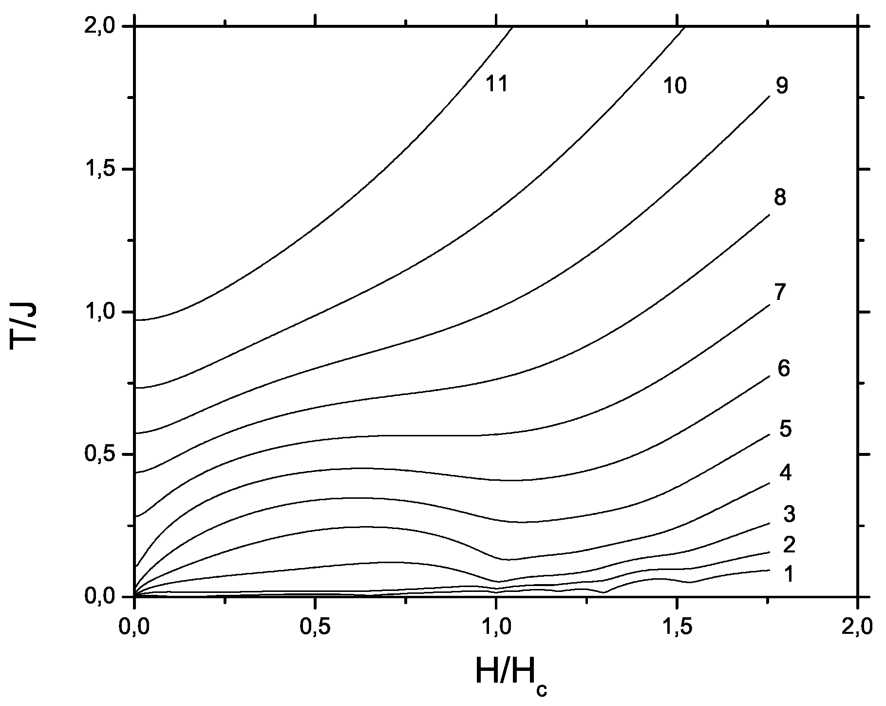
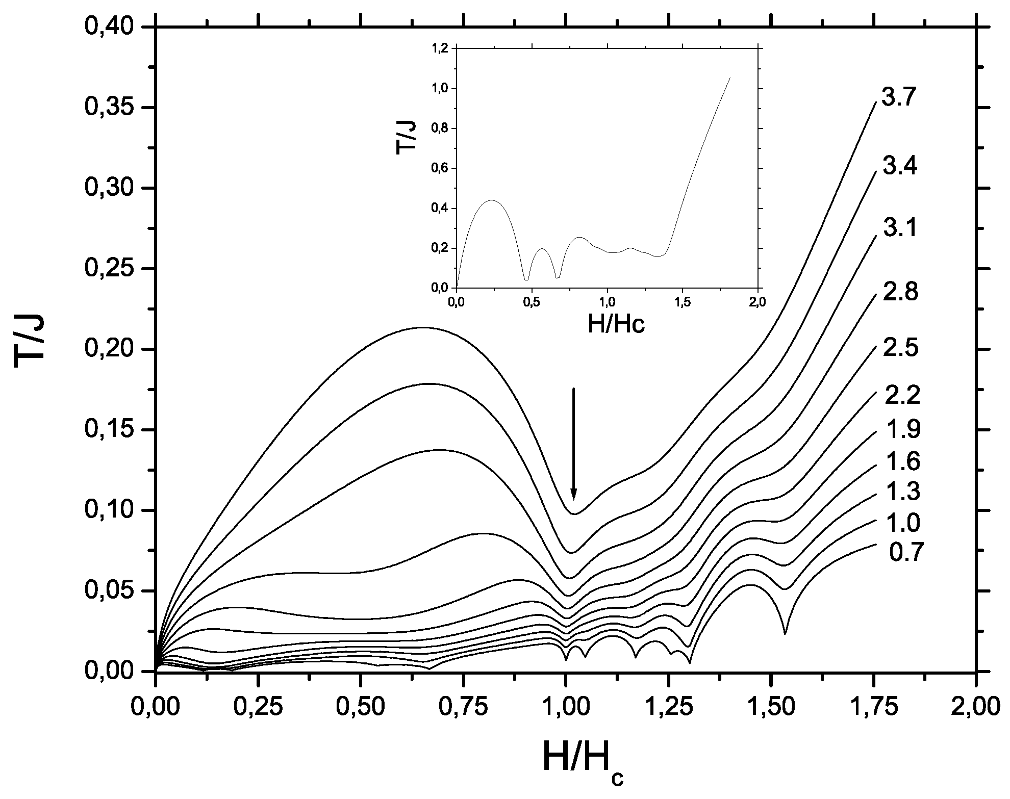
The results are presented in Figure 6 and demonstrate that the isentropes exhibit the expected behavior and they are tilted towards the point $H=H_c$ (the field destroying the ground state plateau) with a minimum in its vicinity. As argued [49,50] the behavior is expected for systems where the finite temperature entropy landscape is determined by an underlying quantum phase transition. A detailed analysis of the quantum criticality is performed [53].

4. Bose-Einstein Condensation in Two-Dimensional Spin-1 Dimerized System

A possibility to study BEC with low-dimensional magnetic materials predicted theoretically twenty 20 years ago [62] gave rise to intense experimental researches in the field. The analogy between the spins and the bosons becomes evident for antiferromagnets where spins form dimers with a spin-singlet ground state [63]. Originally, the attention was mainly focused on spin-1/2 systems, where excitations inside each dimer (triplons) were regarded as bosons with hard-core repulsion, i.e., no more than one boson was presented on a single dimer. The analogy enables to treat spin systems as that of interacting bosons whose ground state is determined by the balance between kinetic energy and repulsive interactions [64]. If the repulsion dominates the bosons form a superlattice and a finite energy cost is needed to create an additional particle. This exhibits itself as a jump in chemical potential versus boson number, in the spin language, as a plateau in magnetization curve versus magnetic field at rational fraction of saturated magnetization. Recently, magnetic weakly coupled dimer system with $S=1$ moments attracted a lot of attention [65,66]. The field behavior of magnetization in the system of antiferromagnetically weakly coupled $S=1$ dimers can be described as BEC of magnons by mapping the spin-1 system into a gas of semi-hard-core bosons [67].

The organic compound F${}_2$PNNNO is an example of spin-one dimer based magnetic insulator [68]. This is 2D Heisenberg system with a singlet ground state, in which $S=1$ dimers interact antiferromagnetically [68,69]. The field magnetization process shows two-step saturation behavior that is a rare example of observing a plateau in a two-dimensional system. The intermediate plateau corresponds to the half value of saturation magnetization. The consistent calculation of susceptibility and magnetization for the finite-size cluster with imposed periodic conditions yields the following estimations of antiferromagnetic exchange couplings $2J_0=67.5$ K, $2J_1=7.5$ K, i.e., the system can be regarded as a real 2D dimerized spin-one system. Apparently, the quantum antiferromagnet F${}_2$PNNNO offers an opportunity to verify a relevance of semi-hard core boson model for description of dimerized system.

The Hamiltonian of weakly interacting spin-one dimers on a 2D lattice depicted in Figure 7 is given by

$$H_S=J_0\sum _i{\overrightarrow{S}}_{i1}{\overrightarrow{S}}_{i2}+J_1\sum _{〈i\alpha ,j\overline{\alpha }〉}{\overrightarrow{S}}_{i\alpha }{\overrightarrow{S}}_{j\overline{\alpha }},$$

(40)

where $J_0$ is the coupling inside the i-th dimer, $J_1$ is the strength of the exchange interaction between the dimers located on the bonds $〈i,j〉$. The indices $\alpha$, $\overline{\alpha }$ mark $S=1$ spins that enter into the interacting dimers, namely, $\overline{\alpha }$ = 1,2 provided $\alpha$ = 2,1, respectively. Both types of the interactions are antiferromagnetic $J_{0,1}>0$, and the regime of weakly interacting dimers, $\left|J_0\right|\gg \left|J_1\right|$, is considered. The Heisenberg model has been previously suggested to explain some thermodynamical properties of F${}_2$PNNNO [68]. Numerical calculations based on the Hamiltonian (40) via exact diagonalization of small clusters and their comparison with experimental data prove its relevance for the ratio $\left|J_1/J_0\right|\ll 1$.

To get the energy spectrum, finite-size clusters composed of $N=10$ and $N=18$ sites are selected. In a choice of the cluster care should be taken to ensure that the lattice point group symmetry is hold. Since intra-dimer interactions are the strongest, the cluster should contain whole dimers and not break them into parts. To mark sites inside the cluster, chessboard-like notations will be used, where site positions along the x axis are marked by numbers whereas positions along the y axis are denoted by Latin letters.

To find eigenfunctions of the cluster that inherit the total cluster spin as a quantum number, we should develop a consecutive procedure for adding spin moments. It is convenient to break the cluster in several parts. Following the strategy of building a cluster used [39], one should identify the central dimer (center) and its environment. The center is composed of $c3$ and $d3$ sites whereas another sites are embodied into environment.

The Hamiltonian of the central dimer has the form $H_c=J_0{\overrightarrow{S}}_{c3}{\overrightarrow{S}}_{d3},$ whereas the interaction between the center and its environment is given by

$$V_{\mathrm{ce}}=J_1{\overrightarrow{S}}_{c3}\left({\overrightarrow{S}}_{c2}+{\overrightarrow{S}}_{c4}\right)+J_1{\overrightarrow{S}}_{d3}\left({\overrightarrow{S}}_{d2}+{\overrightarrow{S}}_{d4}\right).$$

(41)

The environment consists of four parts, namely of two dimers, left (l) and right (r) ones, with the Hamiltonians

$$H_l=J_0{\overrightarrow{S}}_{c1}{\overrightarrow{S}}_{d1},\mathrm{and}{H}_r=J_0{\overrightarrow{S}}_{c5}{\overrightarrow{S}}_{d5},$$

(42)

respectively, as well as two fork-like parts, i.e., the down and upper ones, with the corresponding Hamiltonians

$$H_{\mathrm{down}}=J_0\left({\overrightarrow{S}}_{b2}{\overrightarrow{S}}_{c2}+{\overrightarrow{S}}_{a3}{\overrightarrow{S}}_{b3}+{\overrightarrow{S}}_{b4}{\overrightarrow{S}}_{c4}\right)+J_1{\overrightarrow{S}}_{b3}\left({\overrightarrow{S}}_{b2}+{\overrightarrow{S}}_{b4}\right),$$

(43)

$$H_{\mathrm{up}}=J_0\left({\overrightarrow{S}}_{d2}{\overrightarrow{S}}_{e2}+{\overrightarrow{S}}_{e3}{\overrightarrow{S}}_{f3}+{\overrightarrow{S}}_{d4}{\overrightarrow{S}}_{e4}\right)+J_1{\overrightarrow{S}}_{e3}\left({\overrightarrow{S}}_{e2}+{\overrightarrow{S}}_{e4}\right).$$

(44)

The interaction between the left/right dimers and the fork-like parts is presented as

$$V_{\mathrm{env}}=J_1\left({\overrightarrow{S}}_{c2}{\overrightarrow{S}}_{c1}+{\overrightarrow{S}}_{d2}{\overrightarrow{S}}_{d1}+{\overrightarrow{S}}_{c4}{\overrightarrow{S}}_{c5}+{\overrightarrow{S}}_{d4}{\overrightarrow{S}}_{d5}\right).$$

(45)

The Hamiltonian of the entire cluster gathers all the above terms

$$H=H_c+V_{\mathrm{ce}}+\left\{H_l+H_r+H_{\mathrm{down}}+H_{\mathrm{up}}+V_{\mathrm{env}}\right\}.$$

(46)

There are three states of dimer, an elementary block of the cluster, with total spin $S_{\mathrm{dm}}=0$ (singlet), $S_{\mathrm{dm}}=1$ (triplet), and $S_{\mathrm{dm}}=2$ (quintiplet). The energies of the states are $E_0=-2J_0$, $E_1=-J_0$, $E_2=J_0$, respectively, and the eigenstates are obtained via the common rule of addition of moments

$$\left|11;S_{\mathrm{dm}}{M}_{\mathrm{dm}}\right.〉\equiv \left|S_{\mathrm{dm}}{M}_{\mathrm{dm}}\right.〉=\sum _{{\sigma }_1{\sigma }_2}\left[\begin{array}{ccc}1& 1& S_{\mathrm{dm}}\\ {\sigma }_1& {\sigma }_2& M_{\mathrm{dm}}\end{array}\right]\left|1{\sigma }_1\right.〉\left|1{\sigma }_2\right.〉.$$

(47)

To increase the size of cluster, RMEs of the operators $S\left(1\right)$ and $S\left(2\right)$, that constitute the dimer, calculated within the basis (47), are needed

$$〈S_{\mathrm{dm}}∥S\left(1\right)∥S_{\mathrm{dm}}^{\prime }〉={\left(-1\right)}^{1+S_{\mathrm{dm}}^{\prime }}\sqrt{(2S_{\mathrm{dm}}+1)(2S_{\mathrm{dm}}^{\prime }+1)}\left\{\begin{array}{ccc}{S}_{\mathrm{dm}}& 1& S_{\mathrm{dm}}^{\prime }\\ 1& 1& 1\end{array}\right\}〈1∥S∥1〉,$$

(48)

$$〈S_{dm}∥S\left(2\right)∥S_{dm}^{\prime }〉={\left(-1\right)}^{1+S_{dm}}\sqrt{(2S_{dm}+1)(2S_{dm}^{\prime }+1)}\left\{\begin{array}{ccc}{S}_{dm}& 1& S_{dm}^{\prime }\\ 1& 1& 1\end{array}\right\}〈1∥S∥1〉,$$

(49)

where the RME $〈1∥S∥1〉=\sqrt{6}$.

The fork-like part includes three interacting dimers. It is convenient to build the basis of this fragment according to the scheme $(2+4)+3$ of moment addition, i.e., combining of “prong” dimer functions is followed by adding “handle” function. As a result, basic functions with total spin $S_{\mathrm{down}}$ of the down fork-like part have the form

$$\left|\left(S_2{S}_4\right)S_{24},S_3;S_{\mathrm{down}}{M}_{\mathrm{down}}\right.〉=\sum _{M_2{M}_3{M}_4{M}_{24}}\left[\begin{array}{ccc}{S}_2& S_4& S_{24}\\ M_2& M_4& M_{24}\end{array}\right]\left[\begin{array}{ccc}{S}_{24}& S_3& S_{\mathrm{down}}\\ M_{24}& M_3& M_{\mathrm{down}}\end{array}\right]$$

$$\times \left|S_2{M}_2\right.〉\left|S_3{M}_3\right.〉\left|S_4{M}_4\right.〉,$$

(50)

where $S_2$, $S_3$ and $S_4$ are spins of dimers composed of the $b2$ and $c2$ sites, etc. Within the basis, the Hamiltonian (43) is presented by the block diagonal $141\times 141$ matrix. The blocks are marked by total spin $S_{\mathrm{down}}=0,1,\dots ,6$ values. A diagonalization of $H_{\mathrm{down}}$ matrix yields the spectrum $E_{i_{\mathrm{down}}{S}_{\mathrm{down}}}$ and eigenfunctions

$$\left|i_{\mathrm{down}}{S}_{\mathrm{down}}{M}_{\mathrm{down}}\right.〉=\sum _{S_2{S}_3{S}_4{S}_{24}}{\alpha }_{\left(S_2{S}_4\right)S_{24},S_3}^{i_{\mathrm{down}}{S}_{\mathrm{down}}}\left|\left(S_2{S}_4\right)S_{24},S_3;S_{\mathrm{down}}{M}_{\mathrm{down}}\right.〉,$$

where $i_{\mathrm{down}}$ index distinguishes basic functions with the same total $S_{\mathrm{down}}$ spin. The results for the upper fork-like part can be obtained the same way provided the site $c4$ is substituted for $d2$, and $c2$ is changed by $d4$ etc. The assembly of the cluster part is completed by calculations of RMEs [see Equation (80) in Appendix B].

The next step, we construct the spin functions of the non-interacting parts, i.e., of the left and of the right dimers

$$\left|S_l{S}_r;S_{lr}{M}_{lr}\right.〉=\sum _{M_l{M}_r}\left[\begin{array}{ccc}{S}_l& S_r& S_{lr}\\ M_l& M_r& M_{lr}\end{array}\right]\left|S_l{M}_l\right.〉\left|S_r{M}_r\right.〉,$$

(51)

where $S_{lr}=0,1\dots ,4$, and upper and lower fork-like parts

$$\left|i_{\mathrm{up}}{S}_{\mathrm{up}}{i}_{\mathrm{down}}{S}_{\mathrm{down}};S_{\mathrm{ud}}{M}_{\mathrm{ud}}\right.〉=\sum _{M_{\mathrm{up}}{M}_{\mathrm{down}}}\left[\begin{array}{ccc}{S}_{\mathrm{up}}& S_{\mathrm{down}}& S_{\mathrm{ud}}\\ M_{\mathrm{up}}& M_{\mathrm{down}}& M_{\mathrm{ud}}\end{array}\right]\left|i_{\mathrm{up}}{S}_{\mathrm{up}}{M}_{\mathrm{up}}\right.〉\left|i_{\mathrm{down}}{S}_{\mathrm{down}}{M}_{\mathrm{down}}\right.〉,$$

(52)

where $S_{\mathrm{ud}}=0,1\dots ,12$, and add them together to build the basis of environment for the central dimer

$$\left|\left(i_{\mathrm{up}}{S}_{\mathrm{up}}{i}_{\mathrm{down}}{S}_{\mathrm{down}}\right)S_{\mathrm{ud}},\left(S_l{S}_r\right)S_{lr};S_{\mathrm{env}}{M}_{\mathrm{env}}\right.〉$$

$$=\sum _{M_{\mathrm{ud}}{M}_{lr}}\left[\begin{array}{ccc}{S}_{\mathrm{ud}}& S_{lr}& S_{\mathrm{env}}\\ M_{\mathrm{ud}}& M_{lr}& M_{\mathrm{env}}\end{array}\right]\left|i_{\mathrm{up}}{S}_{\mathrm{up}}{i}_{\mathrm{down}}{S}_{\mathrm{down}};S_{\mathrm{ud}}{M}_{\mathrm{ud}}\right.〉\left|S_l{S}_r;S_{lr}{M}_{lr}\right.〉.$$

(53)

RMEs of spin operators required to build the Hamiltonian of environment are shown in Appendix B [see Equations(81-84)]. Note, that a number of the states (53) is too much to avoid the truncation procedure (see below).

Matrix elements of environment Hamiltonian $H_{\mathrm{env}}=H_l+H_r+H_{\mathrm{down}}+H_{\mathrm{up}}+V_{\mathrm{env}}$ are listed below

$$〈\left(i_{\mathrm{up}}{S}_{\mathrm{up}}{i}_{\mathrm{down}}{S}_{\mathrm{down}}\right)S_{\mathrm{ud}},\left(S_l{S}_r\right)S_{lr};S_{\mathrm{env}}{M}_{\mathrm{env}}\left|H_{\mathrm{env}}\right|\left(i_{\mathrm{up}}^{\prime }{S}_{\mathrm{up}}^{\prime }{i}_{\mathrm{down}}^{\prime }{S}_{\mathrm{down}}^{\prime }\right)S_{\mathrm{ud}}^{\prime },\left(S_l^{\prime }{S}_r^{\prime }\right)S_{lr}^{\prime };S_{\mathrm{env}}^{\prime }{M}_{\mathrm{env}}^{\prime }〉$$

$$=\left(E_{i_{\mathrm{up}}{S}_{\mathrm{up}}}+E_{i_{\mathrm{down}}{S}_{\mathrm{down}}}+E_{S_l}+E_{S_r}\right)$$

$$\times {\delta }_{i_{\mathrm{up}},i_{\mathrm{up}}^{\prime }}{\delta }_{S_{\mathrm{up}},S_{\mathrm{up}}^{\prime }}{\delta }_{i_{\mathrm{down}},i_{\mathrm{down}}^{\prime }}{\delta }_{S_{\mathrm{down}},S_{\mathrm{down}}^{\prime }}{\delta }_{S_{\mathrm{ud}},S_{\mathrm{ud}}^{\prime }}{\delta }_{S_l,S_l^{\prime }}{\delta }_{S_r,S_r^{\prime }}{\delta }_{S_{lr},S_{lr}^{\prime }}{\delta }_{S_{\mathrm{env}},S_{\mathrm{env}}^{\prime }}{\delta }_{M_{\mathrm{env}},M_{\mathrm{env}}^{\prime }}$$

$$+J_1{\delta }_{S_{\mathrm{env}},S_{\mathrm{env}}^{\prime }}{(-1)}^{S_{\mathrm{env}}+S_{\mathrm{ud}}^{\prime }+S_{lr}}\left\{\begin{array}{ccc}{S}_{\mathrm{ud}}& S_{lr}& S_{\mathrm{env}}\\ S_{lr}^{\prime }& S_{\mathrm{ud}}^{\prime }& 1\end{array}\right\}{\delta }_{M_{\mathrm{env}},M_{\mathrm{env}}^{\prime }}$$

(54)

$$\times \left\{〈S_l{S}_r;S_{lr}∥S_{c1}∥S_l^{\prime }{S}_r^{\prime };S_{lr}^{\prime }〉〈i_{\mathrm{up}}{S}_{\mathrm{up}}{i}_{\mathrm{down}}{S}_{\mathrm{down}};S_{\mathrm{ud}}∥S_{c2}∥i_{\mathrm{up}}^{\prime }{S}_{\mathrm{up}}^{\prime }{i}_{\mathrm{down}}^{\prime }{S}_{\mathrm{down}}^{\prime };S_{\mathrm{ud}}^{\prime }〉\right.$$

$$+〈S_l{S}_r;S_{lr}∥S_{d1}∥S_l^{\prime }{S}_r^{\prime };S_{lr}^{\prime }〉〈i_{\mathrm{up}}{S}_{\mathrm{up}}{i}_{\mathrm{down}}{S}_{\mathrm{down}};S_{\mathrm{ud}}∥S_{d2}∥i_{\mathrm{up}}^{\prime }{S}_{\mathrm{up}}^{\prime }{i}_{\mathrm{down}}^{\prime }{S}_{\mathrm{down}}^{\prime };S_{\mathrm{ud}}^{\prime }〉$$

$$+〈S_l{S}_r;S_{lr}∥S_{c5}∥S_l^{\prime }{S}_r^{\prime };S_{lr}^{\prime }〉〈i_{\mathrm{up}}{S}_{\mathrm{up}}{i}_{\mathrm{down}}{S}_{\mathrm{down}};S_{\mathrm{ud}}∥S_{c4}∥i_{\mathrm{up}}^{\prime }{S}_{\mathrm{up}}^{\prime }{i}_{\mathrm{down}}^{\prime }{S}_{\mathrm{down}}^{\prime };S_{\mathrm{ud}}^{\prime }〉$$

$$\left.+〈S_l{S}_r;S_{lr}∥S_{d5}∥S_l^{\prime }{S}_r^{\prime };S_{lr}^{\prime }〉〈i_{\mathrm{up}}{S}_{\mathrm{up}}{i}_{\mathrm{down}}{S}_{\mathrm{down}};S_{\mathrm{ud}}∥S_{d4}∥i_{\mathrm{up}}^{\prime }{S}_{\mathrm{up}}^{\prime }{i}_{\mathrm{down}}^{\prime }{S}_{\mathrm{down}}^{\prime };S_{\mathrm{ud}}^{\prime }〉\right\}.$$

The terms in $\{\dots \}$ include the product of RMEs given by Equations(81,82) for spins that enter into the left/right dimers and by Equations (83,84) for the constituents of the fork-like parts.

After finding environment eigenvalues $E_{i_{\mathrm{env}}{S}_{\mathrm{env}}}$ and eigenfunctions

$$\left|i_{\mathrm{env}}{S}_{\mathrm{env}}{M}_{\mathrm{env}}\right.〉=\sum {\beta }_{\left(i_{\mathrm{up}}{S}_{\mathrm{up}}{i}_{\mathrm{down}}{S}_{\mathrm{down}}\right)S_{\mathrm{ud}},\left(S_l{S}_r\right)S_{lr}}^{i_{\mathrm{env}}{S}_{\mathrm{env}}}\left|\left(i_{\mathrm{up}}{S}_{\mathrm{up}}{i}_{\mathrm{down}}{S}_{\mathrm{down}}\right)S_{\mathrm{ud}},\left(S_l{S}_r\right)S_{lr};S_{\mathrm{env}}{M}_{\mathrm{env}}\right.〉,$$

(55)

one calculate RMEs for the environment spins that directly interact with the central dimer, within the basis (see [Equation (85)]).

As the final step of the diagonalization procedure one build the basis of entire cluster

$$\left|i_{\mathrm{env}}{S}_{\mathrm{env}},S_c;SM\right.〉=\sum _{M_{\mathrm{env}}{M}_c}\left[\begin{array}{ccc}{S}_{\mathrm{env}}& S_c& S\\ M_{\mathrm{env}}& M_c& M\end{array}\right]\left|i_{\mathrm{env}}{S}_{\mathrm{env}}{M}_{\mathrm{env}}\right.〉\left|S_c{M}_c\right.〉,$$

and determine matrix elements of the cluster Hamiltonian (46)

$$〈i_{\mathrm{env}}{S}_{\mathrm{env}},S_c;SM\left|H\right|i_{\mathrm{env}}^{\prime }{S}_{\mathrm{env}}^{\prime },S_c^{\prime };S^{\prime }{M}^{\prime }〉=\left(E_{i_{\mathrm{env}}{S}_{\mathrm{env}}}+E_{S_c}\right){\delta }_{i_{\mathrm{env}},i_{\mathrm{env}}^{\prime }}{\delta }_{S_{\mathrm{env}},S_{\mathrm{env}}^{\prime }}{\delta }_{S_c,S_c^{\prime }}{\delta }_{S,S^{\prime }}{\delta }_{M,M^{\prime }}$$

$$+J_1{\left(-1\right)}^{S+S_{\mathrm{env}}^{\prime }+S_c}\left\{\begin{array}{ccc}{S}_{\mathrm{env}}& S_c& S\\ S_c^{\prime }& S_{\mathrm{env}}^{\prime }& 1\end{array}\right\}{\delta }_{S,S^{\prime }}{\delta }_{M,M^{\prime }}$$

$$\times \left[〈S_c∥S\left(1\right)∥S_c^{\prime }〉\sum _{k=c2,c4}〈i_{\mathrm{env}}{S}_{\mathrm{env}}∥S_k∥i_{\mathrm{env}}^{\prime }{S}_{\mathrm{env}}^{\prime }〉+〈S_c∥S\left(2\right)∥S_c^{\prime }〉\sum _{k=d2,d4}〈i_{\mathrm{env}}{S}_{\mathrm{env}}∥S_k∥i_{\mathrm{env}}^{\prime }{S}_{\mathrm{env}}^{\prime }〉\right],$$

(56)

where RMEs are previously derived [see Equations(48-49) and Equation (85)]. Numerical diagonalization of the matrix (56) yields target spectrum $E_{iS}$ and eigenfunctions

$$\left|iSM\right.〉=\sum {\gamma }_{S_{\mathrm{env}}{M}_{\mathrm{env}},S_c}^{iS}\left|S_{\mathrm{env}}{M}_{\mathrm{env}},S_c;SM\right.〉.$$

(57)

The classification of eigenstates of parts we used to gather the total cluster according to irreducible representations of $SU\left(2\right)$-group enables us to organize truncation procedure inside sectors of Hilbert space that arise at consecutive steps of the algorithm. A possibility to carry out calculations within reduced basis is feature of the algorithm that relates it with other renormalization group methods.

We hold the following strategy of truncation procedure to build target states that are obtained after combining two parts of lattice. For given spin-S sector a certain amount of states having the lowest energies are kept. Thus each group of $\left|iS\right.〉$ states is presented in reduced basis. We truncate the basis of two “fork”-like parts before combining them into a larger lattice segment. This is not the only way to do so, for example one can truncate the basis of environment after combining the “fork”-like parts, but the former is easier to perform.

We tested several realizations of truncation procedure either by simply controlling a number of vectors retained in the reduced basis or by monitoring a genealogy of the target spin-S state through the triangle rule, i.e., only states that contribute into the target state are taken into account. The last approach gives an opportunity to keep more vectors in the basis due to omitting of redundant states. Moreover, the highest-spin cluster states, i.e., those with $S\ge 15$ in our problem, are treated exactly. The size of truncated basis was chosen equal to either 64 or 121 for the scheme without taking genealogy of the target state into account, and it varies from 12 till 352, being dependent on the total spin S, for the “genealogical” scheme.

An accuracy of truncation procedure is controlled by monitoring an energy of the lowest state within each spin sector. The variation of this observable computed through the both schemes does not normally exceed 1-2% (a maximum discrepancy of order 6% is reached only in the S-8 sector) that provides an evidence for the correctness of constructed basis, which exhibits almost no dependence on the used truncation procedure. The results that we present below are obtained within the “genealogical” scheme.

Another feature of the algorithm is combining central unit (one site or dimer) with its environment at the final step. The procedure does not depend on the structure of environment and looks similar for any cluster. However, the information about quantum numbers of the environment states enables to simplify calculations substantially at this stage of the algorithm. Indeed, for given spin-S sector of Hilbert space of entire cluster one should pick out only those environment eigenfunctions which spins $S_u$ obey the rule

$$|S_u-S_c|\le S\le S_u+S_c.$$

Using of truncation procedure results in basises composed maximum from 4–5 thousand states. To control accuracy of the procedure, results obtained for the 18-site system are compared with those for the 10-site system. The smaller cluster enables to handle the complete basis without any truncation. The 10-site system is embedded into bigger cluster and consists of the following parts: the central dimer $c3,d3$ and neighbor dimers $b2,c2$, $b4,c4$, $d2,e2$ and $d4,e4$. Apparently, a construction of environment requires two consecutive steps (i) addition of dimers $b2,c2$ and $b4,c4$ as well as $d2,e2$ and $d4,e4$ ones according to Equation (51) followed by calculation of RMEs according to Equations (81,82); (ii) construction of the environment states from upper and lower parts built previously and calculation of RME of the environment spins that interact directly with the central dimer. The entire cluster Hamiltonian is obtained through (56). The biggest Hilbert space dimension ($2025\times 2025$) is reached in S-2 sector. Numerical results for the supplementary cluster are listed in

Table 6. Numerical results of the lowest energy $E_{min}$ and the energy $\tilde{\epsilon }$ per dimer in the spin-S subspaces for $N=10$ and $N=18$ clusters.

S	$E_{min}(N=10)/J_0$	$\tilde{\epsilon }(N=10)$	$E_{min}(N=18)/J_0$	$\tilde{\epsilon }(N=18)$
0	−10.0334	−2.0067	−18.0336	−2.0037
1	−9.1853	−1.8371	−17.1431	−1.9048
2	−8.2123	−1.6425	−16.2529	−1.8059
3	−7.1978	−1.4396	−15.2935	−1.6993
4	−6.1430	−1.2286	−14.3205	−1.5912
5	−4.9344	−0.9869	−13.3164	−1.4796
6	−2.9787	−0.5957	−12.2745	−1.3638
7	−0.9610	−0.1922	−11.1879	−1.2431
8	1.0849	0.2170	−10.0260	−1.1140
9	3.1588	0.6318	−8.8335	−0.9815
10	5.4418	1.0883	−6.8807	−0.7645
11			−4.8994	−0.5444
12			−2.8795	−0.3199
13			−0.8172	−0.0908
14			1.2815	0.1424
15			3.4533	0.3837
16			5.6844	0.6316
17			7.960	0.8844
18			10.3254	1.1473

for comparison. Note that one should compare energy values with the same magnetization per dimer (See Figure 8).

The results of energy spectrum calculation for two $N=10$ and $N=18$ clusters are listed in Table 6, where minimal energy $E_{min}$ within each spin-S sector along with energy per dimer $\tilde{\epsilon }=2E_{min}/N$ are given. The magnetization per dimer is determined by $m=2S/N$. Both $N=10$ and $N=18$ dependencies $\tilde{\epsilon }\left(m\right)$ are shown together in Figure 8. Points for both clusters lay on the same curve, i.e., finite-size effects can be ignored which is expected for the regime of a small dimer-dimer interaction $J_1\ll J_0$.

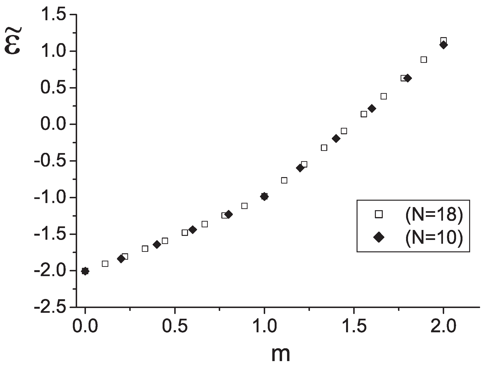
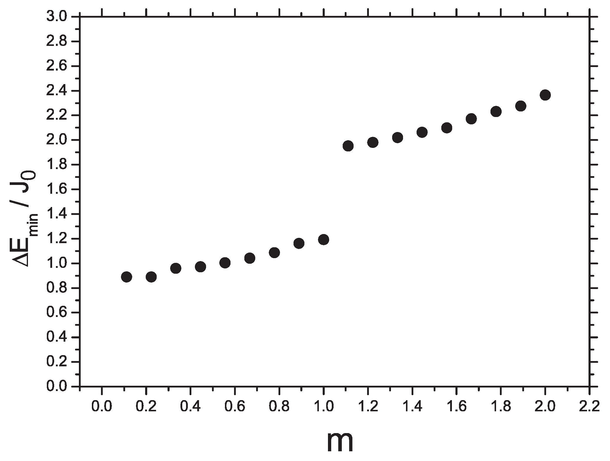
A remarkable feature of the curve is the cusp in the middle, i.e., at $m=1$. Independent fitting of both parts by the quadratic form $\epsilon \left(m\right)={\epsilon }_2{m}^2+{\epsilon }_{1}m+{\epsilon }_0$ jointed in the point yields ${\epsilon }_2=0.190\pm 0.018$, ${\epsilon }_1=0.828\pm 0.019$, and ${\epsilon }_0=-2.0073\pm 0.0040$ for lower part of the curve ($0<m<1$) together with ${\epsilon }_2=0.200\pm 0.058$, ${\epsilon }_1=1.4578\pm 0.018$, and ${\epsilon }_0=-2.629\pm 0.014$ for upper part ($1<m<2$).

Based on $N=18$ case data we build a dependence of jumps $E_{min}$ when the total spin S changes from 0 till 18, or the dimer magnetization varies from 0 till 2 (Figure 9) One can see that the values of jumps are approximately $J_0$ for $S\le 9$ and they increase by a factor of 2 as $S\ge 10$. It means that the energy of the total system of weakly interacting dimers changes with an increase of magnetic field due to local excitations inside separate dimers. Indeed, for the single $S=1$ dimer the spectrum consists of a singlet, a triplet, and a quintuplet. The energy difference between the singlet and the triplet is $J_0$ while the difference between the quintuplet and the triplet is $2J_0$.

A standard way to describe magnetization process at $T=0$ is to define $E_{min}^{\left(S\right)}\left(N\right)$ as the lowest energy of the Hamiltonian (40) in the spin-S subspace for the finite system of N elementary dimers. Applying magnetic field B leads to the Zeeman splitting of energy levels $E_{min}^{\left(S\right)}\left(B\right)=E_{min}^{\left(S\right)}-SB$, and therefore, the level crossing occurs at values $B_S=E_{min}^{(S+1)}\left(B\right)-E_{min}^{\left(S\right)}\left(B\right)$ when the field is increasing. These level crossings correspond to jumps of value $1/N$ in magnetization at zero temperature, until the fully polarized state with magnetization per dimer $m_{\mathrm{sat}}=2N/N=2$ is reached at value of the magnetic field $B_{\mathrm{sat}}=E_{min}^{\left(2N\right)}\left(B\right)-E_{min}^{(2N-1)}\left(B\right)$. 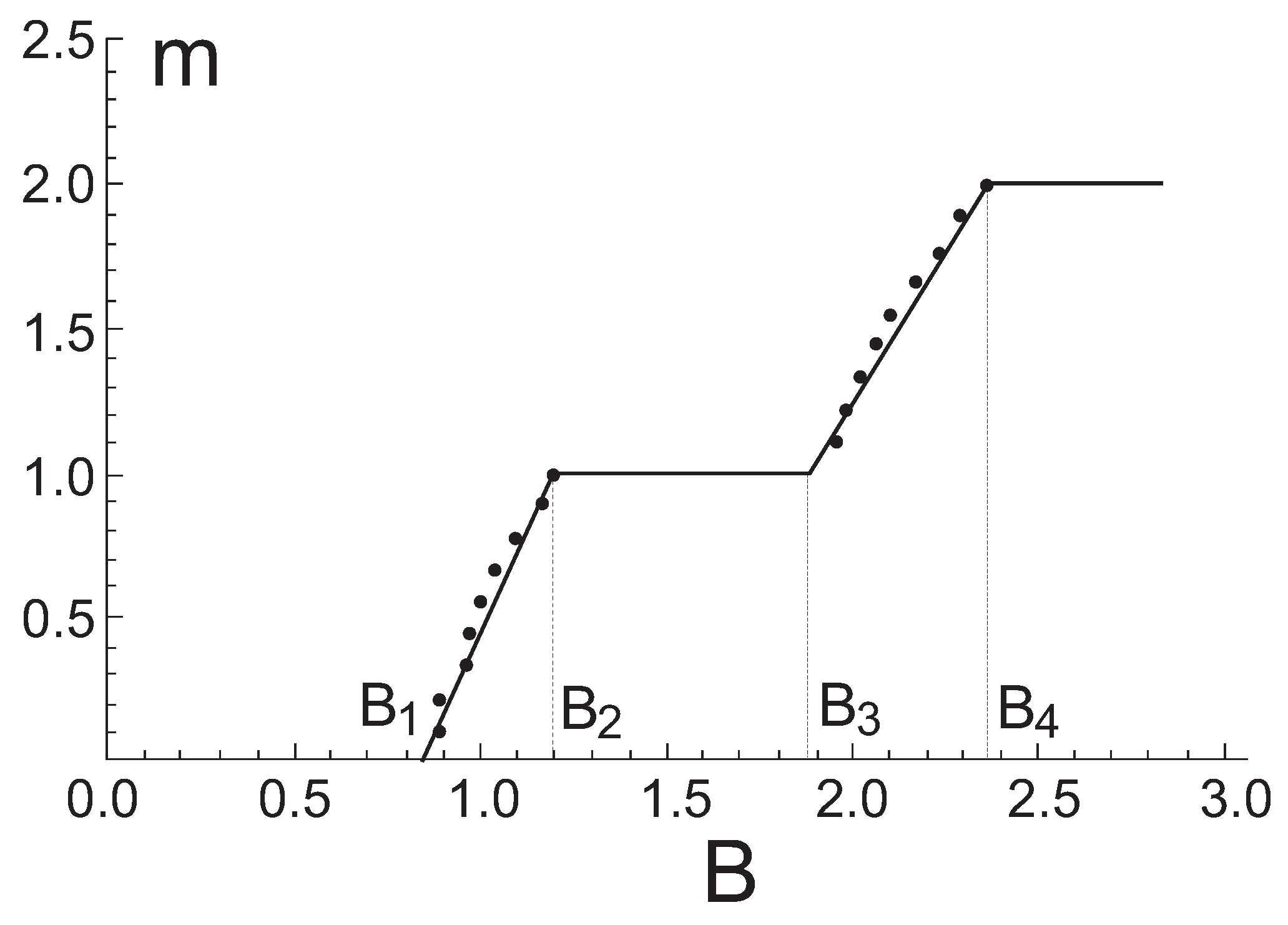The calculation performed for $N/2=9$ dimers yields the magnetization points presented in Figure 10 and reveals the appearance of the ground state plateau as well as the plateau at one-half of the saturation value.

To guarantee the validity of the magnetization curve we use the approach developed by Sakai and Tahakashi [70] to recover the $m\left(B\right)$ dependence in thermodynamical limit. In this case the condition for crossover fields transforms into $B={\epsilon }^{\prime }\left(m\right)$, where $\epsilon$ is the energy per dimer. The plateau boundaries are determined by the derivatives in the special points: (i) $B_1={\epsilon }^{\prime }(+0)$ is related with the end of the ground state plateau; (ii) $B_2={\epsilon }^{\prime }(1-0)$ and $B_3={\epsilon }^{\prime }(1+0)$ correspond to the beginning and the end of intermediate plateau, respectively; (iii) $B_4={\epsilon }^{\prime }(2-0)$ marks an emergence of saturation magnetization.

Treating the energy spectrum results in linear dependences relevant to the sectors between plateaus

$$\left\{\begin{array}{c}{\epsilon }^{\prime }\left(m\right)=0.83+0.38m,0<m<1,\\ {\epsilon }^{\prime }\left(m\right)=1.46+0.40m,1<m<2,\end{array}\right.$$

(58)

that yields immediately $B_1=0.83J_0$, $B_2=1.21J_0$, $B_3=1.86J_0$, and $B_4=2.26J_0$. Values normalized to the saturation field $B_{\mathrm{sat}}$ are listed in

Table 7. Values of the magnetic field special points compared with the experimental data [68].

$B_i/B_{\mathrm{sat}}$	i = 1	i = 2	i = 3	i = 4
$\mathrm{Theory}$	0.37	0.53	0.82	1
$\mathrm{Experiment}$	0.33	0.53	0.89	1

and exhibit a reasonable agreement with the experimental data for F${}_2$PNNNO system. A comparison of finite cluster calculations with those of thermodynamical limit (58) is given in Figure 10. One can see that both methods come to the close results.

Note that the method we used for numerical calculations is intrinsically two-dimensional one whereas the previous numerical study of the system [68] dealt with essentially one-dimensional “folded chain” cluster. The regions between the plateaus of the magnetization curve exhibit a behavior closer to linear one instead of the S-shape forms obtained earlier.

The data presented in Figure 9 enable to introduce the boson picture. For $J_1\ll J_0$ the low energy subspace of spin Hamiltonian (40) consists of the singlet, the $S^z=1$ component of the triplet, and the $S^z=2$ component of the quintuplet. It is convenient to identify the triplet state with the presence of a bosonic particle (triplon), the quintiplet state as a pair of bosons (quintuplon), and the singlet state as an absence of bosons. 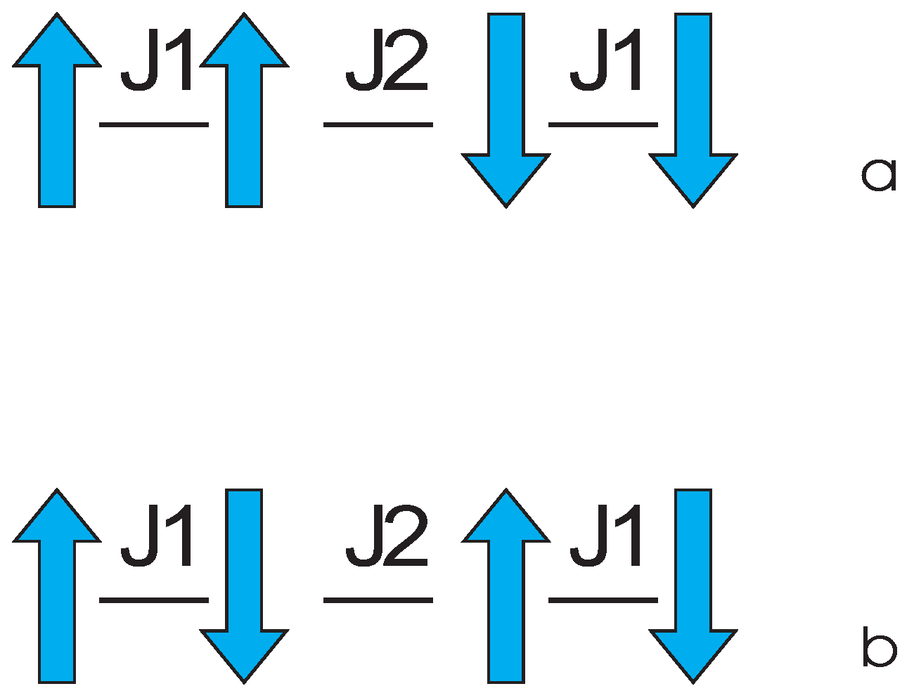Then, the boson model is formulated via the semi-hard core bosonic operators $g_i$ and $g_i^{†}$ with the extended Pauli’s exclusion principle $g_i^{†3}=0$, i.e., more then two bosons per site are forbidden [71,72]. According to this study, the magnetization curve shown in Figure 10 can be interpreted as tuning of boson density by applied magnetic field. At small chemical potential, the lowest energy is achieved by empty states, i.e., those where all dimers are in the singlet state (boson vacuum). For $B>B_1$ a finite density of bosons (triplons) emerges in the ground state and contributes into Bose-superfluid (BS) phase. The triplon excitations are mobile due to weak interdimer coupling. The density (magnetization) increases monotonically as a function of magnetic field until $B_2$, where transition to charge ordering (CO) phase comes up. 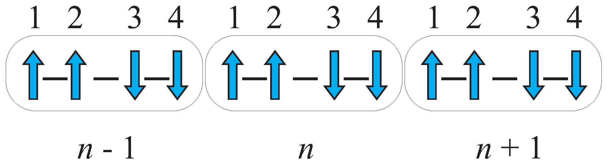This corresponds to the boson concentration $n=0.5$, when the triplons crystallize in a superstructure pattern (Figure 11). The fractional plateau requires strong boson interactions in comparison to the kinetic energy. At $B>B_3$ the filling increases monotonically in resulting BS phase (quintiplon condensation) until the ground state transforms into Mott insulating (MI) phase with two bosons per dimer at $B>B_4$.

5. Cluster Perturbation Theory

In last ten years, the quantum cluster methods became effective tool in studies of lattice quantum models. Nowadays they are widely applied along with the ED and QMC methods. The various modern cluster methods, i.e., the variational cluster perturbation theory (VCPT) [73], the cluster theory of dynamical mean field [74], the method of dynamical cluster approximation [75], deal with a lattice cluster of finite size embedded into the infinite lattice, where the cluster environment is modeled either by auxiliary fields, or by heat bath additional degrees of freedom. In contrast to conventional mean field theory, these methods are dynamical and completely account of correlation effects [76].

The simplest of the cluster methods is the cluster perturbation theory (CPT) [77,78,79], which is a constituent part of the contemporary VCPT. Below, we consider an extension of the theory to quantum spin system. We calculate the magnon spectral function for two spin-1/2 chains with the Hamiltonian

$$\mathcal{H}=J_1\sum _{i=1}^{N/2}{\mathbf{S}}_{2i-1}{\mathbf{S}}_{2i}+J_2\sum _{i=1}^{N/2}{\mathbf{S}}_{2i}{\mathbf{S}}_{2i+1}.$$

The Hamiltonian includes two types of alternative exchange couplings between the nearest neighbors (Figure 12). In the limit $|J_2/J_1|\ll 1$, the first chain belongs the class of Haldane systems with a gap in the spin-wave excitation spectrum (it is equivalent to spin-1 antiferromagnet at $J_1\to \infty$). The second chain is the dimerized spin-1/2 chain which is of interest due to possible observation of BEC in low-dimensional magnetic materials [62,64].

The both compounds has a singlet ground state, however in the first case we deal with a Haldane liquid phase, i.e., the liquid with antiferromagnetic order without positional order. In the liquid the hidden order is featured by non-local string order parameter. Elementary excitations presents singlet-triplet excitations (spinon) traveled along the chain. In the second case elementary excitations are the local singlet-triplet excitations (triplon) localized inside the dimers. These excitations can be mapped onto boson particles either with an intersite attraction ($J_2<0$) or repulsion ($J_2>0$).

The main idea of the cluster perturbation theory is to divide the lattice into a superlattice of identical clusters. As a next step one should calculate the spin Green function within the each cluster. Interactions between the clusters are perturbatively treated. The Lanczos algorithm based on the information about a ground state of the cluster is a conventional way to calculate the cluster Green function [17]. An alternative way to get the quantity is to use Lehmann’s representation based on the cluster energy spectrum and wavefunctions.

The Hamiltonian treated in the CPT can be splitted in two parts

$$H=H_0+V,$$

(59)

where

$$H_0=\sum _{\mathbf{R}}{H}_{\mathbf{R}}^0$$

is the sum of cluster Hamiltonians,

$$V=\sum _{\mathbf{R},{\mathbf{R}}^{\prime }}{V}_{ab}^{\mathbf{R},{\mathbf{R}}^{\prime }}{\mathbf{S}}_{\mathbf{R}a}{\mathbf{S}}_{{\mathbf{R}}^{\prime }b}$$

is the sum of intercluster interactions. Here, a and b mark spins inside the cluster, for example, a and b equal to either 1 or 4 as shown in Figure 13. In this case, $V_{ab}^{\mathbf{R},{\mathbf{R}}^{\prime }}$ is the exchange coupling between spin a of the cluster $\mathbf{R}$ and spin b of the cluster ${\mathbf{R}}^{\prime }$.

Firstly, we describe how to calculate the cluster Green function ${\widehat{G}}_{ab}$ by means of $SU\left(2\right)$ group formalism [80]. In an absence of anisotropic terms in a Hamiltonian, the elementary excitation spectrum is determined by Matsubara’s pair Green function of transversal

$$G_{ab}^{-+}\left(\tau \right)=-\frac{1}{2}\langle \widehat{T}{S}_a^{-}\left(\tau \right)S_b^{+}\left(0\right)\rangle ,$$

(60)

and longitudinal fluctuations

$$G_{ab}^{zz}\left(\tau \right)=-\langle \widehat{T}\left(S_a^z\left(\tau \right)-\langle S_a^z\rangle \right)\left(S_b^z\left(0\right)-\langle S_b^z\rangle \right)\rangle =-\langle \widehat{T}{S}_a^z\left(\tau \right))S_b^z\left(0\right)\rangle .$$

(61)

We took into account that in the singlet ground state $\langle S_{a,b}^z\rangle =0$.

At zero temperature Lehmann’s representation of the Green function (60) is given by

$$G_{ab}^{-+}\left(\omega \right)=\sum _m\frac{\langle 0|{\widehat{S}}_a^{-}|m\rangle \langle m|{\widehat{S}}_b^{+}|0\rangle }{\omega +i\eta -E_m+E_0},$$

(62)

where $|0\rangle$ and $|m\rangle$ are the wave functions of the ground and excited cluster states with the energies $E_0$ and $E_m$, respectively.

According to Wigner-Eckart theorem the matrix elements in Lehmann representation (62) have the form

$$\langle 0|{\widehat{S}}_a^{-}|m\rangle ={(-1)}^{0-0}\left(\begin{array}{ccc}0& 1& 1\\ 0& -1& 1\end{array}\right)\langle 0∥{\widehat{S}}_a∥m\rangle =\frac{1}{\sqrt{3}}\langle 0∥{\widehat{S}}_a∥m\rangle ,$$

(63)

where m marks the cluster excited states of spin 1. Then the cluster Green function is simplified to

$${\widehat{G}}_{ab}\left(\omega \right)=\frac{1}{3}\sum _m\frac{\langle 0∥{\widehat{S}}_a∥m\rangle \langle m∥{\widehat{S}}_a∥0\rangle }{\omega +i\eta -E_m+E_0}.$$

(64)

To obtain the cluster energies $E_m$ and the RMEs the exact diagonalization method with an account of $SU\left(2\right)$ symmetry can be used [81]. We briefly sketch the recursion scheme to calculate the RMEs of spins at the positions a and b.

At given step of iterations the cluster consists of two blocks of n sites, i.e., left (l) and right (r) ones. To start the iterations, it is reasonably to take a pair of dimers whose eigensystem is easily determined. By using the angular momentum addition rule the basis functions of the entire system are constructed

$$|(i_l{S}_l,i_r{S}_r)SM\rangle =\sum _{m_l{m}_r}\left[\begin{array}{ccc}{S}_l& S_r& S\\ m_l& m_r& M\end{array}\right]|i_l{S}_l{m}_l\rangle |i_r{S}_r{m}_r\rangle ,$$

(65)

where $i_l$($i_r$) indicates the states of the left (right) block with the same quantum numbers $S_l$, $m_l$ ($S_r$, $m_r$).

The Hamiltonian matrix of the interaction blocks is built through Wigner-Eckart theorem

$$\begin{array}{c}\langle (i_l{S}_l,i_r{S}_r);SM\left|\widehat{H}\right|(i_l^{\prime }{S}_l^{\prime },i_r^{\prime }{S}_r^{\prime });S^{\prime }{M}^{\prime }\rangle =\end{array}=(E_{i_l{S}_l}+E_{i_r{S}_r}){\delta }_{i_l{S}_l,i_l^{\prime }{S}_l^{\prime }}{\delta }_{i_r{S}_r,i_r^{\prime }{S}_r^{\prime }}{\delta }_{S,S^{\prime }}{\delta }_{M,M^{\prime }}+$$

(66)

$$+J_2{(-1)}^{S_l^{\prime }+S_r+S}\left\{\begin{array}{ccc}{S}_r& S_l& S\\ S_l^{\prime }& S_r^{\prime }& 1\end{array}\right\}{\delta }_{S,S^{\prime }}{\delta }_{M,M^{\prime }}\langle i_l{S}_l\Vert S_{ln}\Vert i_l^{\prime }{S}_l^{\prime }\rangle \langle i_r{S}_r\Vert S_{r1}\Vert i_r^{\prime }{S}_r^{\prime }\rangle .$$

The corresponding eigenfunctions are easily found

$$|iSM\rangle =\sum _{i_l{S}_l{i}_r{S}_r{m}_l{m}_r}{\alpha }_{i_l{S}_l{i}_r{S}_r}^{iS}|(i_l{S}_l,i_r{S}_r)SM\rangle .$$

(67)

The RME of the block edge spins $S_{r1}$ and $S_{ln}$ interacting directly with each other have been determined at the previous iteration step.

We apply repeatedly Wigner-Eckart theorem and calculate the RMEs within the basis of the extended cluster of the length $2n$. For the sites $a=1,\dots n$ that enter in the left part we obtain

$$\begin{array}{c}\langle iS\Vert S_a\Vert i^{\prime }{S}^{\prime }\rangle =\\ ={[S,S^{\prime }]}^{1/2}{(-1)}^{1+S^{\prime }}\sum {\alpha }_{i_l{S}_l{i}_r{S}_r}^{iS}{\alpha }_{i_l^{\prime }{S}_l^{\prime }{i}_r^{\prime }{S}_r^{\prime }}^{i^{\prime }{S}^{\prime }}{\delta }_{i_r^{\prime },i_r}{\delta }_{S_r^{\prime },S_r}{(-1)}^{S_l+S_r}\left\{\begin{array}{ccc}S& 1& S^{\prime }\\ S_l^{\prime }& S_r& S_l\end{array}\right\}\langle i_l{S}_l\Vert S_a\Vert i_l^{\prime }{S}_l^{\prime }\rangle .\end{array}$$

(68)

The corresponding results for the sites $a=n+1,\dots 2n$ at the right parts are given by

$$\begin{array}{c}\langle iS\Vert S_a\Vert i^{\prime }{S}^{\prime }\rangle =\\ ={[S,S^{\prime }]}^{1/2}{(-1)}^{1+S}\sum {\alpha }_{i_l{S}_l{i}_r{S}_r}^{iS}{\alpha }_{i_l^{\prime }{S}_l^{\prime }{i}_r^{\prime }{S}_r^{\prime }}^{i^{\prime }{S}^{\prime }}{\delta }_{i_l^{\prime },i_l}{\delta }_{S_l^{\prime },S_l}{(-1)}^{S_l+S_r^{\prime }}\left\{\begin{array}{ccc}S& 1& S^{\prime }\\ S_r^{\prime }& S_l& S_r\end{array}\right\}\langle i_r{S}_r\Vert S_{a-n}\Vert i_r^{\prime }{S}_r^{\prime }\rangle ,\end{array}$$

(69)

where $\left[S\right]=2S+1$.

Following the same route it can be demonstrated that the Green function of the longitudinal fluctuations (61) differs from the expression (64) only by sign. Without anisotropic interactions this is explained by degeneration of the triplet states over the spin projections. The fact differs singlet magnets from systems with ordered local moments. In the last case relevant excitations at low temperatures are spin waves described by the Green function of the transversal fluctuations. A contribution of longitudinal spin excitations becomes noticeable at a critical region, i.e., near a temperature of magnetic ordering.

In an approximation of the nearest neighbors the interaction term is given by the complex $L\times L$ matrix

$${\widehat{V}}_{ab}^{\mathbf{R},{\mathbf{R}}^{\prime }}=J_2\left({\delta }_{a,L}{\delta }_{b,1}{\delta }_{{\mathbf{R}}^{\prime },\mathbf{R}+1}+{\delta }_{a,1}{\delta }_{b,L}{\delta }_{{\mathbf{R}}^{\prime },\mathbf{R}-1}\right),$$

that has the Fourier transform

$${\widehat{V}}_{ab}\left(Q\right)=J_2\left({\delta }_{a,L}{\delta }_{b,1}{e}^{iQLa}+{\delta }_{a,1}{\delta }_{b,L}{e}^{-iQLa}\right)$$

(70)

in the reduced Brillouine zone BZ${}_{\Gamma }$ (Brillouine zone of the superlattice). Here, a and $La$ are lattice constants of the initial lattice and superlattice, respectively.

An account of the interaction within the perturbation theory yields the “dressed” Green function

$${\widehat{\mathcal{G}}}_{ab}(\mathbf{Q},\omega )={\left[\frac{\widehat{G}\left(\omega \right)}{1-\widehat{V}\left(\mathbf{Q}\right)\widehat{G}\left(\omega \right)}\right]}_{ab}.$$

(71)

Equation (71) is given in the mixed representation of the real space inside the cluster and of the reciprocal space for the intercluster distances. The Fourier representation in terms of wave vectors $\mathbf{k}$ of the initial Brillouine zone BZ${}_{\gamma }$ is more preferable. To reach this the wave vector $\mathbf{k}$ is decomposed as follows

$$\mathbf{k}=\mathbf{K}+\mathbf{Q},$$

(72)

where $\mathbf{Q}$ belongs to the reduced Brillouine zone BZ${}_{\Gamma }$, and the vector $\mathbf{K}$ does to the reciprocal superlattice ${\Gamma }^{*}$.

A transition to the translationally invariant Green function is given by the transformation

$${\mathcal{G}}_{\mathrm{CPT}}(\mathbf{k},\omega )=\frac{1}{L}\sum _{a,b=1}^L{\mathcal{G}}_{ab}(\mathbf{Q},\omega )e^{-i\mathbf{k}({\mathbf{r}}_a-{\mathbf{r}}_b)},$$

(73)

where ${\mathcal{G}}_{ab}(\mathbf{k},\omega )$ is invariant under the translations $\mathbf{K}$ within the reciprocal superlattice.

The spectral function of elementary excitations is determined as follows [79]

$$A(\mathbf{k},\omega )=-2\underset{\eta \to 0^{+}}{lim}\mathrm{Im}{\mathcal{G}}_{\mathrm{CPT}}(\mathbf{k},\omega +i\eta ),$$

and the corresponding density of states equals to

$$\mathcal{N}\left(\omega \right)=\frac{1}{N}\sum _{\mathbf{k}}A(\mathbf{k},\omega ),$$

where N is a number of lattice sites.

Firstly, we present the CPT calculations for the cluster composed of 4 sites. To get peaks of finite width we take $\eta$=0.01. The wave vector k varies within a half of the Brillouine zone $k\in [0,\pi /a]$. The vector $Q\in [0,\pi /4a]$ belonging to the reduced Brillouine zone can be found through Equation (72), where $\mathrm{K}$ is one of the reciprocal superlattice vectors $\left\{0,\pi /4a,\pi /2a,3\pi /4a\right\}$.

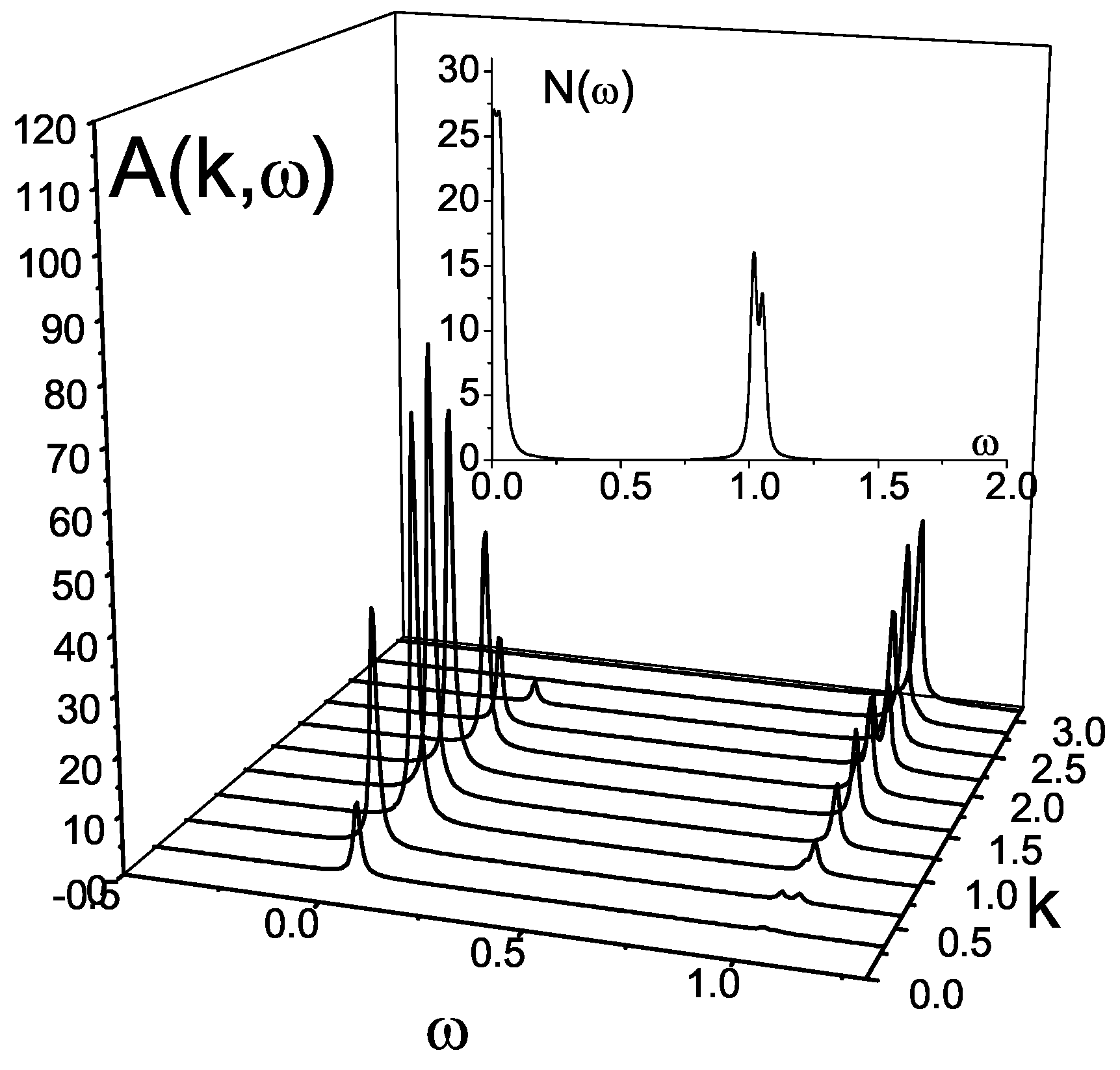
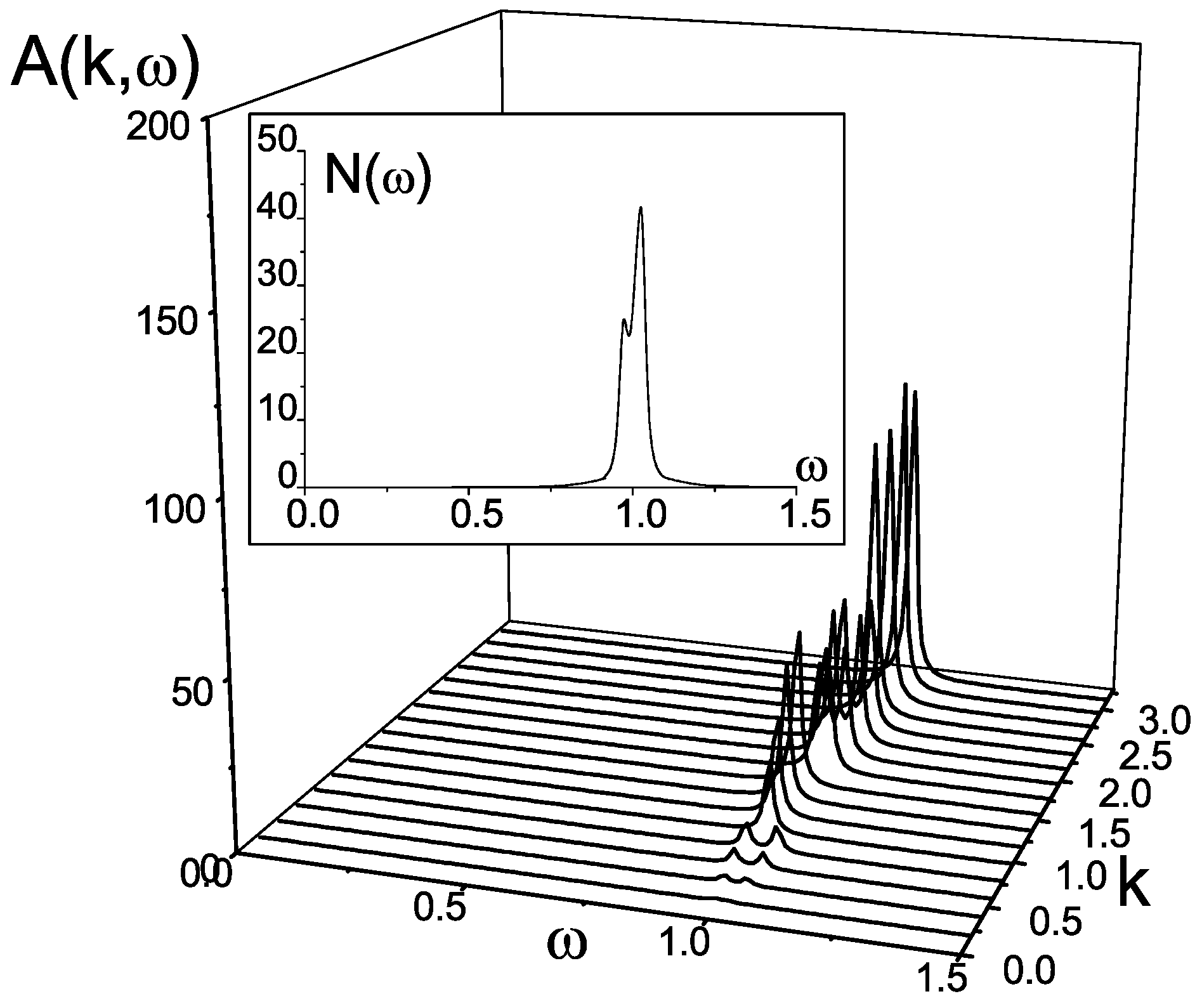
The plot (Figure 14) of the spectral function $A(k,\omega )$ of the first type chain (Figure 12a) demonstrates an appearance of two spinon branches in the excitations spectrum of Haldane’s antiferromagnetic liquid regime ($J_2/J_1=-0.07$). The corresponding density of states possesses two-peak structure.

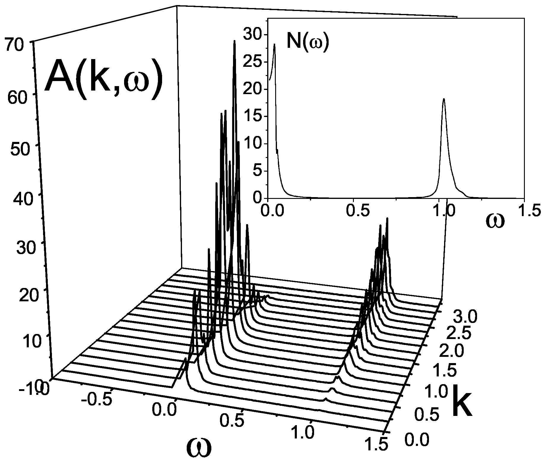
The case of the dimerized chain (Figure 12b) results in another picture of the spectral function (Figure 15). There is only one dispersionless branch of singlet-triplet excitations around $\omega \approx J_1$ corresponding to excitations of bosonic type localized inside the dimer. The maximum of the intensity $A(k,\omega )$ falls on the BZ edge. The density of states exhibits one-peak structure.

Being related with an infinite chain the results for the spectral function and the density of states contain finite-size effects since the Green function $\widehat{G}\left(\omega \right)$ is built for a finite cluster. To elucidate finite-size effects we repeat the CPT calculations for a cluster of bigger size, and taking, for example, the chain of the first type. For the case $L=8$ the result of such calculations is presented in Figure 16. Despite an appearance of subtleties in the density of states, a direct comparison of the spectral functions $A(k,\omega )$ for the clusters of $L=4$ and $L=8$ sizes demonstrates that the size-effects can be ignored.

In conclusion, we emphasize that a relevant description of spectral properties within the perturbation theory must be supported by a small parameter of the theory. In our case, the ratio $J_2/\left(J_{1}L\right)$, where L is the cluster length, plays the role of the small quantity. As a result, an increasing of the inter-dimer interaction $J_2$ must be accompanied by a simultaneous increasing of a minimal cluster size. This may invoke the $SU\left(2\right)$ symmetry based procedure of a basis truncation similar to those used in the previous Sections.

6. Conclusion

In summary, the main results of the quantum mechanical applications of the symmetry concepts in low-dimensional magnetism are reviewed. The treatment is based on the irreducible tensor operator technique and the group-theoretical classification provided both the $SU\left(2\right)$ spin-symmetry and the lattice point symmetry. The flexibility of the method was demonstrated for several one-dimensional and two-dimensional spin models. The use of the symmetries allows to essentially reduce the matrices of Hamiltonians and facilitate evaluation of the excitation spectrum and thermodynamic properties of low-dimensional magnets. The group-theoretical classification might be crucial for efficient truncation of Hilbert space in algorithms based on real-space renormalization group procedure. The applications clearly exhibit that the symmetry concepts are indispensable in the field of low-dimensional magnetism.