
Low-Order Moments of Velocity Gradient Tensors in Two-Dimensional Isotropic Turbulence

1
Laboratory of Complex System, Ecole Centrale de Pékin/School of General Engineering, Beihang University, Beijing 100191, China
2
The State Key Laboratory of Nonlinear Mechanics, Institute of Mechanics, Chinese Academy of Sciences, Beijing 100190, China
3
School of Engineering Sciences, University of Chinese Academy of Sciences, Beijing 100049, China
*
Author to whom correspondence should be addressed.
Symmetry 2024, 16(2), 175; https://doi.org/10.3390/sym16020175
Submission received: 30 December 2023
/
Revised: 24 January 2024
/
Accepted: 28 January 2024
/
Published: 1 February 2024
(This article belongs to the Special Issue Applications Based on Symmetry/Asymmetry in Fluid Mechanics)
Abstract
:In isotropic turbulence, symmetry of different directions can reduce the number of independent components for velocity gradient tensors. In three-dimensional isotropic turbulence, the independent components under either incompressible or compressible conditions have already been analyzed in the literature. However, for two-dimensional isotropic turbulence, they are still unclear. We derive rigorously the independent components for velocity gradient tensors of two-dimensional isotropic turbulence and give physical explanations. These theoretical results are validated using high-resolution direct numerical simulations (DNSs) of two-dimensional compressible turbulence. Results show that the present DNS setup is still not sufficient to capture the isotropy of third-order moments, suggesting that more investigations on determining the smallest scale and improving the numerical schemes for two-dimensional compressible turbulence are required.
1. Introduction
Homogeneous and isotropic turbulence (HIT) is the simplest type of turbulent flow. It provides a cornerstone for us to study more complex turbulence systems. For example, the local isotropy assumption for small-scale dynamics is one of the main hypotheses in the celebrated K41 theory [1,2], from which we could obtain the important energy spectrum, the four-fifth law for third-order structure functions, etc. In the small-scale dynamics of turbulence, the velocity gradient tensor (or in component form, where denotes the velocity) characterize the local flow pattern. For example, the deformation and rotational motion can be described by the symmetric part and the anti-symmetric part of , where and [3,4,5]. Specifically, the second-order moments of the velocity gradient , defined as , describe the strength of the local motions, like the enstrophy , which describes the strength of local rotational motion, where is the vorticity vector and is the Levi-Civita symbol. Furthermore, the viscosity dissipation in turbulence, , with , the kinematic viscosity, is obviously determined by . Then, in the dynamic equation of the second-order moment , the third-order moment of the velocity gradient appears due to the nonlinearity of the Navier–Stokes equation. These third-order moments determine the key nonlinear process such as the vortex stretching rate [3,5,6], which is crucial for the generation of small-scale motions in turbulence. As a consequence, a complete understanding of the properties of the moments of the velocity gradient is important in the studies of small-scale dynamics of turbulence. In this work, we will focus on the kinematics properties of and , especially their invariants and independent components.
Betchov’s relation is one of the important theoretical results in the studies of kinematic properties of velocity gradients. In 1956, Betchov derived two constraints on the second- and third-order invariants of for homogeneous and incompressible flows [7]. In three-dimensional (3D) isotropic incompressible turbulence, with the help of Betchov’s relations, we can determine all the components of and with, respectively, only one scalar quantity [8,9]. Recently, Yang et al. [10] generalized the Betchov’s relation to compressible turbulence and showed that one needs two and four scalars to fully determine and , respectively, in isotropic compressible turbulence. Furthermore, we note that Carbone and Wilczek [11] have proved that Betchov’s relations are the only constraints on the invariants of the velocity gradient under the homogeneity condition. In addition to the second- and third-order moments, the structure of higher-order moments, such as fourth-order, has also been studied previously for 3D homogeneous incompressible and compressible turbulence [12,13,14].
Up to now, most studies on the velocity gradient focus on 3D turbulence. At the same time, a reduction in dimensionality leads to the emergence of new phenomena. For example, in two-dimensional (2D) incompressible HIT, all components of the third-order moments are equal to zero because of the absence of vortex stretching [15,16,17]. This results in the conservation of enstrophy and a net energy transfer from small to large scales, which is known as the inverse energy cascade [18,19]. Furthermore, 2D isotropic compressible turbulence exhibits distinct phenomena, such as the energy flux loop between incompressible and compressible components [20]. However, to the best of our knowledge, the structure of the velocity gradient in 2D turbulence, especially in the compressible case, is yet to be explored. The current studies on 2D compressible turbulence [20,21,22,23] are rather phenomenological and mainly focus on the dual cascade of energy and enstrophy, as well as the interchange of energy between the dilation and divergence-free parts in the spectral space. There is still no strict theory explaining the energy transfer and energy flux loop. We recall that in 3D isotropic incompressible turbulence, the energy transfer can be represented by using the Kármán–Howarth equation, in which the analysis of independent scalars plays an essential role. A study of the velocity gradient tensor in this case would be beneficial for understanding the local flow motion and energy transfer in 2D turbulence.
In this work, we investigate the structure of the velocity gradient tensor in 2D turbulence, including the components of its low-order moments, i.e., and , and the corresponding invariants, e.g., , . The rest of the paper is structured as follows. In Section 2, we present the theoretical derivations, focusing first on the decomposition of velocity gradient tensor , and then using the isotropy and homogeneity constraints to determine the independent components of low-order moments. Furthermore, we express the second- and third-order invariants in terms of these independent components and explain the underlying physical meaning of them. The above theoretical derivation is verified in Section 3 by direct numerical simulations (DNSs) of 2D homogeneous and isotropic compressible turbulence. Finally, in Section 4 we give further discussions on the analytical relations and the numerical results.
2. Analytical Studies on the Components of Velocity Gradient Tensors in 2D Turbulence
2.1. Decomposition of the Velocity Gradient Tensor
In general, the velocity gradient tensor can be decomposed into dilatational, symmetric-deviatoric, and antisymmetric parts, as follows:
where is the dilatational part with and n is the dimension of the flow field. Here, for simplicity, we used the overbar symbol to denote the trace operation: . The tensor is the deviatoric part of the rate-of-strain tensor:
where is the transpose of the tensor. The tensor is the antisymmetric rate-of-rotation tensor defined as in the introduction, which can be equivalently expressed by the vorticity vector with .
In a 3D space generated by an orthogonal basis , if the flow is confined in the plane , then the velocity gradient tensor can be decomposed as:
where are four independent components of the local velocity gradient tensor, and the subscripts of each matrix means that the matrix is expressed in the basis. More precisely, and are defined as and , respectively, which represent the local shear motion of the flow. denotes the vorticity and because of the constraints from 2D space, it only has the components, i.e., , where . Finally, denotes the dilatation as mentioned above.
For 2D homogeneous turbulence, the four independent components are locally independent, but they are globally related in spectral space. This relation is shown in Appendix A.
2.2. Isotropic Expressions for and
Under the isotropic condition, second- and third-order moments of the velocity gradient, and , can be expressed, respectively, as the following [9]:
where is the Kronecker tensor ( if , and 0 otherwise), and and are scalar quantities.
These two formulas generally hold in 2D and 3D (or even in higher-dimension flows, which do not exist physically). However, if the flow is confined to 2D, the subscripts in Equations (4) and (5), (), can choose only from two different values, 1 and 2. As the second-order moment has the specific form shown in Equation (4), its components would be non-zero only if there are even numbers of 1 and even numbers of 2 among the four subscripts . As a consequence, there are only four types of non-zero components of , as shown in Table 1. For example, if a second-order moment has the form , such as with and with , its value will be . This can be shown by setting all subscripts in Equation (4) to 1 or 2.
Similarly, is non-zero only if there are even numbers of 1 and even numbers of 2 among the six subscripts . We should also note that the indices pairs are interchangeable due to the symmetry of . thus has four non-zero types of components, as shown in Table 2. For example, , and all belong to the same type , as the first two are just the cases and , and the third because the indices pairs and are interchangeable. Thus, from Equation (5), these three components all have the same value .
It can be shown from Table 2 that
Thus, for 2D compressible isotropic turbulence, could be fully determined by three scalars, i.e., , and . It should be remarked that this is only applicable in 2D and are all indeed independent in 3D or in higher dimensions. This derivation is a novel process in 2D that has not been and can not be applied in 3D cases to reduce the independent components.
Next, in Table 3 and Table 4, we express the second- and third-order invariants in terms of the scalars in Equations (4) and (5). In these two tables, the first column gives the tensor notation of the invariants and the second column gives the corresponding subscript representation in terms of the components of and . By substituting Equation (3) into the definitions of the invariants, i.e., the expressions in the first columns of those tables, we could obtain the expression of these invariants in terms of , the results of which are presented in the third columns of Table 3 and Table 4. Furthermore, with the help of Equations (4) and (5), we can express these invariants in terms of the scalars, and , which is shown in the fourth columns of those tables.
The identifications in Table 3 and Table 4 also allow us to make a connection between the independent scalars and . For the second-order values,
For the third-order values,
The identifications in Table 4 and Equations (8a)–(8c) are also consistent with the limiting case when the turbulence is incompressible, i.e., . The left-hand side of Equations (8a)–(8c) will all be zero and will lead to:
As a result, velocity gradient skewness is zero for 2D incompressible isotropic flows.
2.3. Homogeneity Constraints to Second- and Third-Order Invariants
According to Yang et al. [10], under the homogeneity condition, i.e., , one can obtain two invariants relation for second- and third-order moments of velocity gradient, i.e.,
For the second-order invariant, by substituting the results of Table 3 into Equation (10), we have:
As a result, the second-order velocity gradient moment only has two independent components. From Equations (7a)–(7c), we can show that:
which could also be proved from the spectral approach—see Equation (A13) in the Appendix A. This shows the consistency between independent scalar analysis and spectral space analysis.
However, if we combine Table 4 and Equation (11) for the third-order invariants, we find that Equation (11) is automatically satisfied without giving any new constraint to . This is different from the 3D case analysed by Yang et al. [10], where Equation (11) gives a new constraint to the five independent components. This shows that the constraints on independent components for the third-order moment are from different sources. In the 2D case, the constraints are from isotropy, while in the 3D case, the constraints are from the homogeneity. Consequently, copying simply the same method of 3D tensor derivation in reference [10] will lead to incorrect independent scalars and will result in a contraction that the third-order moment has more independent components in 2D than in 3D.
We also note that is positive definite (), thus, from Equations (7a) and (12), we can readily show that , and the equal sign holds when , that is, the incompressible case. Similarly, as , from Equations (7c) and (12), we have , and the equal sign holds when the flow is irrotational. These two inequalities provide restrictions on the ratio between the components of :
The minimum and maximum of the ratio are achieved, respectively, at irrotational flow and incompressible flow.
3. Numerical Validation of Independent Components
To verify the theoretical results presented above, we performed a 2D compressible isotropic DNS. We numerically solve the following two-dimensional compressible Navier–Stokes equations:
in which is the density, p is the pressure, is the total energy with , the ratio of the specific heats, is the viscous stress tensor with the effect of bulk viscosity neglected [24], and is the heat flux. The ideal gas law is applied in calculation to connect the temperature T, pressure p, and density through the ideal gas law, and R is the ideal gas constant. The viscosity is connected with the local temperature through Sutherland’s law with , and constants. The thermal conductivity is determined from the viscosity by a constant Prandtl number , with being the specific heat at constant pressure.
In terms of the numerical methods, the set of Equations (15a)–(15c) are solved with a high-order finite difference method. Specifically, the convective terms are calculated by a seventh-order low-dissipative monotonicity-preserving scheme [25] such that shock waves in a compressible flow can be captured and the capabilities of resolving small-scale turbulent structures are preseved. The diffusion terms are discretized by a sixth-order compact central scheme [26] with a domain decoupling scheme for parallel computation [27]. The time integration is computed by a three-step third-order total variation diminishing Runge–Kutta method [28]. For the flow solution of the present study, we use an open-source solver called ASTR (The code is accessible in https://github.com/astr-code/astr (accessed on 30 December 2023)). This solver has been widely validated in DNSs of various compressible turbulent flows with and without shock waves [10,14,25,29,30,31].
The flow we study is a decaying flow. The computational domain is a square domain discretized with a uniform grid. Periodic boundary conditions are applied in both directions. The initial velocity field is divergence-free with a spectrum . The maximum wavenumber is set at to include both directions of the 2D dual-cascade effect in the simulation. The initial kinetic energy is determined by a constant A. The density, pressure, and temperature are all initialized to constant values. The divergence-free nature of the initial velocity field leads to the emergence of strong compression during the initial stage before transitioning to a stable decaying state. To measure the compressibility, we use the turbulent Mach number, which is defined basing on the root-mean-square velocity and the speed of sound , i.e., . Its initial value is set as . Figure 1a shows the evolution of . Except for a small fluctuation during the initial stage, decreases continuously to about at the end of the simulation. In terms of the time normalization, we adopt the initial large-eddy-turnover time . Throughout the simulation, the Kolmogorov scale first decreases and then increases continuously once the turbulent regime is well-established. The minimum Kolmogorov scale verifies with being the grid size; therefore, the flow is well-resolved down to the dissipation scale.
The inset of Figure 1a represents the evolution of the skewness of the longitudinal velocity gradient, calculated as . Figure 1b shows the evolution of the kinetic energy normalized by its initial value , the enstrophy normalized by its initial value , and the average squared dilatation normalized by its maximum value . The latter is defined similarly to enstrophy to show the compressibility effect. These figures illustrate the flow field evolution. In the initial stage, a strong compression emerges due to the divergence-free uniform-density initial condition, leading to a rapid increase in the average squared dilatation , a sharp decrease in the enstrophy , and a distinct negative peak in the skewness . Both and reach their extrema at . The flow field attains a relatively stable state after , from which point, the skewness becomes stable with small oscillations between and . The kinetic energy , the enstrophy , and the average squared dilatation all show a smooth decaying curve caused by the viscous dissipation. Notably, and decay more rapidly than the kinetic energy .
In the following paragraphs, we will calculate the quantities relating to velocity gradients to validate the analytical results in Section 2.
Figure 2 shows the time evolution of quantities relating to the independent components of the second-order moments. Figure 2a shows the equality of and normalized by the average squared Frobenius norm of the velocity gradient tensor . The initial value of (and ) reaches the incompressible limit of , which can be proved by using Table 3 and Equation (7a)
Figure 2b shows the evolution of the ratio , which should lie between and 3 according to Equation (14). The initial value reaches the incompressible limit value 3.
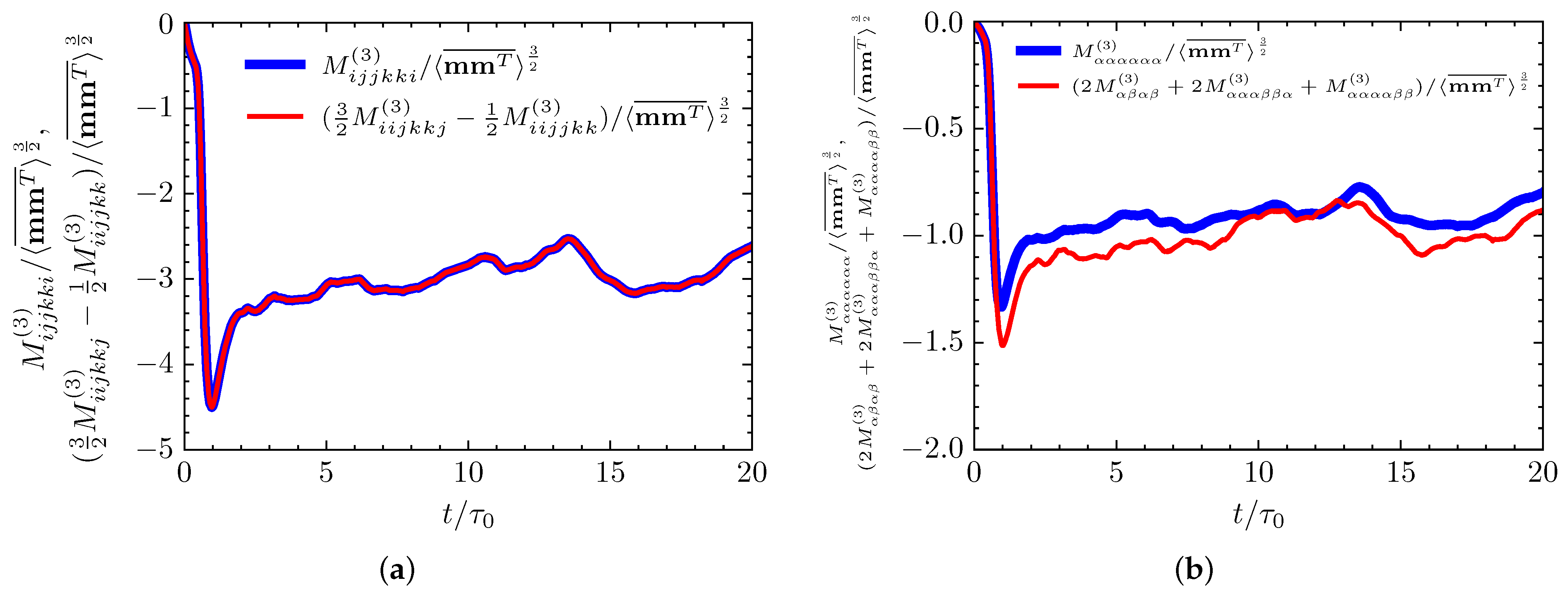
Figure 3 shows the time evolution of quantities relating to the second-order invariants or moments of the velocity gradient tensor. The evolution of the third-order invariants and is presented in Figure 3a, normalized by . The equality in Equation (11), obtained by homogenous constraints, is validated perfectly. For Equation (6), the time evolution of the left-hand side, i.e., , and of the right-hand side, i.e., , is presented in Figure 3b. Their values are both normalized by . To mitigate directional bias, each type of velocity gradient moment is computed by considering all possible expressions. For instance, is calculated using . In Figure 3b, both values exhibit similar trends and fall to the same level, but slight differences occur occasionally. These small disagreements are due to the strict isotropy condition required for Equation (6), which is difficult to achieve numerically. In compressible flow, strong local shocks are likely to occur and cause local anisotropy, as a single shock can only be oriented in a specific direction; while global isotropy is theoretically attainable in a sufficiently large flow field, practical limitations emerge due to bounded domains and finite grid sizes, resulting in unavoidable random anisotropy in numerical results. This random anisotropy leads to disagreements in results requiring isotropic conditions. In particular, third-order moments of the velocity gradient are more sensitive than second-order moments, since they are more influenced by rare but extreme values of the local velocity gradient. These extreme values are exactly caused by local strong shocks. As our DNS is performed by the exact use of classical numerical criteria, i.e., the grid resolution set to with the Kolmogorov length, in this sense, the present analytical study on the moments of the velocity gradient tensor reveals the limitation of current numerical methods in capturing isotropy of third-order moments in 2D compressible turbulence. This calls for more investigations on the smallest scale of two-dimensional compressible turbulence and the numerical schemes of shock capturing in the future.
4. Conclusions
In this paper, we analyze the independent components of the second- and third-order moments of the velocity gradient tensor in 2D isotropic turbulence. The second-order moments have two independent components in the 2D compressible isotropic turbulence, which is the same as in the 3D case. However, as an example of the effect of dimension reduction, the third-order moments could be fully determined by three independent components in 2D isotropic compressible turbulence, while in 3D we need four. This fact leads to an important result that the third-order moments disappear when the flow is incompressible in 2D. From the perspective of small-scale generation, which is closely related to the third-order moments of the velocity gradient, the difference between the number of independent components for 2D and 3D is a consequence of the absence of vortex stretching in two-dimensional flows. We expect that the present study on the independent scalars in 2D isotropic compressible turbulence will represent a step toward rigorously explaining the energy transfer in the future.
We further demonstrate those analytical discussions by numerical simulations. We find that all theoretical results are satisfied by the DNS data except Equation (6), where we see small discrepancies between the l.h.s. and r.h.s. of the equation. This observation is novel and shows that the isotropy of third-order moment of the velocity gradient is not satisfied, such that the derived exact relation, i.e., Equation (6), cannot be obtained by a classical DNS numerical setup. The underlying reason for this might due to the inappropriate prediction on the smallest scale of two-dimensional compressible turbulence, or the inappropriate numerical schemes of shock capturing, which requires future improvement in numerical simulations of HIT. Our result is thus expected to be a criterion for examining the appropriate resolution of small-scale structures and the isotropy of the turbulence field.
Author Contributions
Conceptualization, L.F.; methodology, P.-F.Y. and L.F.; software, C.L.; validation, C.L.; formal analysis, C.L.; investigation, C.L. and P.-F.Y.; resources, L.F.; writing—original draft preparation, C.L.; writing—review and editing, P.-F.Y. and L.F.; visualization, C.L.; supervision, P.-F.Y. and L.F.; project administration, L.F.; funding acquisition, P.-F.Y. and L.F. All authors have read and agreed to the published version of the manuscript.
Funding
This work was supported by the National Natural Science Foundation of China (Project Approval Nos. 12372214 and 12202452) and the Science Center for Gas Turbine Project (Grant No. P2022-C-III-001-001).
Data Availability Statement
For more specific information about the simulated data, please email Le Fang at [email protected].
Conflicts of Interest
The authors declare no conflicts of interest. The funders had no role in the design of the study; in the collection, analyses, or interpretation of data; in the writing of the manuscript; or in the decision to publish the results.
Appendix A. The Relation of θ, ω, ψ, ϕ in Fourier Space
In this appendix, we will show the global relation of the locally independent velocity gradient components, i.e., , in the Fourier space.
In a 3D space generated by an orthogonal basis , where the flow is confined in the plane , we first apply the Helmholtz decomposition to the velocity field , as
where denotes the Fourier transform of the velocity field, denotes the unit vector in the direction of wave vector , and denotes the unit vector with which an orthogonal right-hand coordinate system can be formed. In this equation, and represent, respectively, the solenoidal and the dilatational component of the velocity fluctuation field. The component of is exactly the ensemble average of velocity field
which will be dropped out in the following text as it will not contribute to the velocity gradient. It is also worth noting that the solenoidal component can only follow one direction, i.e., , in 2D, while in 3D, it can be in the Craya plane and gives two independent components.
The counterpart of the velocity gradient tensor in Fourier space can be expressed as
Furthermore, we set . Specifically, the vorticity and the dilatation in Fourier space can be uniquely expressed as
The velocity field can also be expressed as
As a result, the velocity gradient tensor in Fourier space can be expressed with only and
The Fourier space velocity gradient tensor can also be decomposed into dilatational, symmetric-deviatoric, and antisymmetric parts. When it is expressed in the global basis , it can result in a similar expression to Equation (3) with . However, when we express it in the local wave-number basis , it gives
It should be noted that is a local basis. For different wave numbers , unless they are in the same direction, and give two different bases. If we carry out a change of basis for Equation (A8) to , we can derive for
with being the coordinate of in direction. These two equations link and , showing the consistency between different decompositions.
It can also be concluded from Equations (A9) and (A10) that
and also verifies this equation. With an integral in the whole wave number space and Parseval’s identity, this leads to
In the case of homogeneous turbulence, we then obtain
which is also proved in Equation (13) using the independent components of the second-order moment.
References
- Kolmogorov, A. Dissipation of energy in locally isotropic turbulence. Dokl. Akad. Nauk SSSR 1941, 32, 16–18. [Google Scholar]
- Kolmogorov, A. The local structure of turbulence in incompressible viscous fluid for very large Reynolds numbers. Dokl. Akad. Nauk SSSR 1941, 30, 301–305. [Google Scholar]
- Tsinober, A. An Informal Conceptual Introduction to Turbulence; Springer: Berlin/Heidelberg, Germany, 2009. [Google Scholar] [CrossRef]
- Meneveau, C. Lagrangian Dynamics and Models of the Velocity Gradient Tensor in Turbulent Flows. Annu. Rev. Fluid Mech. 2011, 43, 219–245. [Google Scholar]
- Davidson, P.A. Turbulence: An Introduction for Scientists and Engineers; Oxford University Press: Oxford, UK, 2015. [Google Scholar] [CrossRef]
- Taylor, G.I. The spectrum of turbulence. Proc. R. Soc. Lond. Ser. A-Math. Phys. Sci. 1938, 164, 476–490. [Google Scholar] [CrossRef]
- Betchov, R. An inequality concerning the production of vorticity in isotropic turbulence. J. Fluid Mech. 1956, 1, 497–504. [Google Scholar] [CrossRef]
- Champagne, F.H. The fine-scale structure of the turbulent velocity field. J. Fluid Mech. 1978, 86, 67–108. [Google Scholar] [CrossRef]
- Pope, S.B. Turbulent Flows; Cambridge University Press: Cambridge, UK, 2000. [Google Scholar]
- Yang, P.F.; Fang, J.; Fang, L.; Pumir, A.; Xu, H. Low-order moments of the velocity gradient in homogeneous compressible turbulence. J. Fluid Mech. 2022, 947, R1. [Google Scholar] [CrossRef]
- Carbone, M.; Wilczek, M. Only two Betchov homogeneity constraints exist for isotropic turbulence. J. Fluid Mech. 2022, 948, R2. [Google Scholar] [CrossRef]
- Siggia, E.D. Invariants for the one-point vorticity and strain rate correlation functions. Phys. Fluids 1981, 24, 1934–1936. [Google Scholar] [CrossRef]
- Hierro, J.; Dopazo, C. Fourth-order statistical moments of the velocity gradient tensor in homogeneous, isotropic turbulence. Phys. Fluids 2003, 15, 3434–3442. [Google Scholar] [CrossRef]
- Fang, L.; Zhang, Y.; Fang, J.; Zhu, Y. Relation of the fourth-order statistical invariants of velocity gradient tensor in isotropic turbulence. Phys. Rev. E 2016, 94, 023114. [Google Scholar] [CrossRef] [PubMed]
- Tabeling, P. Two-dimensional turbulence: A physicist approach. Phys. Rep. 2002, 362, 1–62. [Google Scholar] [CrossRef]
- Clercx, H.; van Heijst, G. Two-Dimensional Navier–Stokes Turbulence in Bounded Domains. Appl. Mech. Rev. 2009, 62, 020802. [Google Scholar] [CrossRef]
- Boffetta, G.; Ecke, R.E. Two-dimensional turbulence. Annu. Rev. Fluid Mech. 2012, 44, 427–451. [Google Scholar] [CrossRef]
- Kraichnan, R.H. Inertial ranges in two-dimensional turbulence. Phys. Fluids 1967, 10, 1417–1423. [Google Scholar] [CrossRef]
- Kraichnan, R.H. Inertial-range transfer in two- and three-dimensional turbulence. J. Fluid Mech. 1971, 47, 525–535. [Google Scholar] [CrossRef]
- Falkovich, G.; Kritsuk, A.G. How vortices and shocks provide for a flux loop in two-dimensional compressible turbulence. Phys. Rev. Fluids 2017, 2, 092603. [Google Scholar] [CrossRef]
- Dahlburg, J.; Dahlburg, R.; Gardner, J.; Picone, J. Inverse cascades in two-dimensional compressible turbulence. I. Incompressible forcing at low Mach number. Phys. Fluids A Fluid Dyn. 1990, 2, 1481–1486. [Google Scholar] [CrossRef]
- Alexakis, A.; Biferale, L. Cascades and transitions in turbulent flows. Phys. Rep. 2018, 767–769, 1–101. [Google Scholar] [CrossRef]
- Fouxon, I.; Kritsuk, A.G.; Mond, M. Compressible two-dimensional turbulence: Cascade reversal and sensitivity to imposed magnetic field. New J. Phys. 2023, 25, 113005. [Google Scholar] [CrossRef]
- Pan, S.; Johnsen, E. The role of bulk viscosity on the decay of compressible, homogeneous, isotropic turbulence. J. Fluid Mech. 2017, 833, 717–744. [Google Scholar] [CrossRef]
- Fang, J.; Li, Z.; Lu, L. An optimized low-dissipation monotonicity-preserving scheme for numerical simulations of high-speed turbulent flows. J. Sci. Comput. 2013, 56, 67–95. [Google Scholar] [CrossRef]
- Lele, S.K. Compact finite difference schemes with spectral-like resolution. J. Comput. Phys. 1992, 103, 16–42. [Google Scholar] [CrossRef]
- Fang, J.; Gao, F.; Moulinec, C.; Emerson, D. An improved parallel compact scheme for domain-decoupled simulation of turbulence. Int. J. Numer. Methods Fluids 2019, 90, 479–500. [Google Scholar] [CrossRef]
- Gottlieb, S.; Shu, C.W. Total variation diminishing Runge–Kutta schemes. Math. Comput. 1998, 67, 73–85. [Google Scholar] [CrossRef]
- Fang, J.; Yao, Y.; Li, Z.; Lu, L. Investigation of low-dissipation monotonicity-preserving scheme for direct numerical simulation of compressible turbulent flows. Comput. Fluids 2014, 104, 55–72. [Google Scholar] [CrossRef]
- Fang, J.; Yao, Y.; Zheltovodov, A.A.; Li, Z.; Lu, L. Direct numerical simulation of supersonic turbulent flows around a tandem expansion-compression corner. Phys. Fluids 2015, 27, 125104. [Google Scholar] [CrossRef]
- Fang, J.; Zheltovodov, A.A.; Yao, Y.; Moulinec, C.; Emerson, D.R. On the turbulence amplification in shock-wave/turbulent boundary layer interaction. J. Fluid Mech. 2020, 897, A32. [Google Scholar] [CrossRef]
Figure 1.
(a) Time evolution of the turbulent Mach number and the skewness of the longitudinal velocity derivative (shown in inset). (b) Time evolution of the kinetic energy normalized by its initial value , the enstrophy normalized by its initial value and the average squared dilatation normalized by its maximum value .
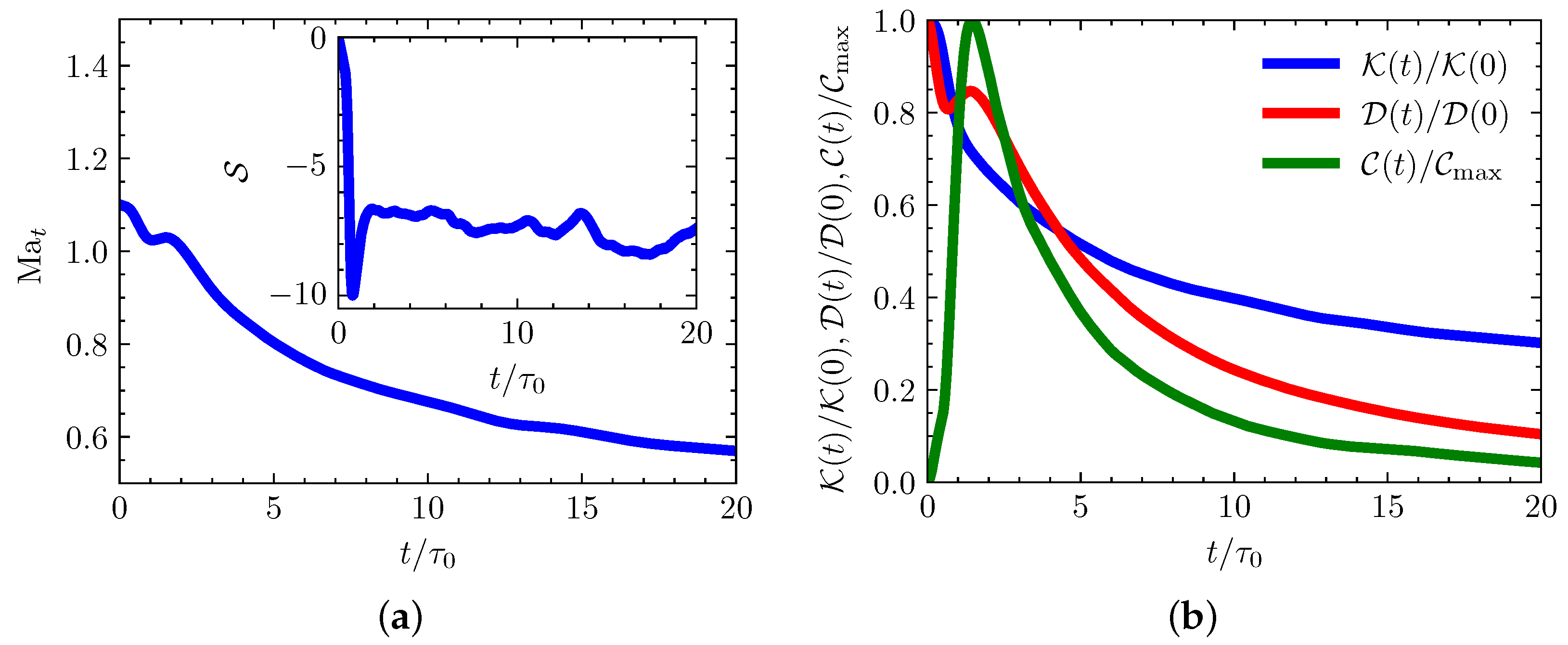
Figure 2.
(a) Time evolution of second-order independent components and normalized by , which should be equal in 2D isotropic compressible turbulence. The dashed line in black is . (b) Time evolution of the ratio , which should lie between and 3 in 2D isotropic turbulence. The dashed lines in black are, respectively, and 3.
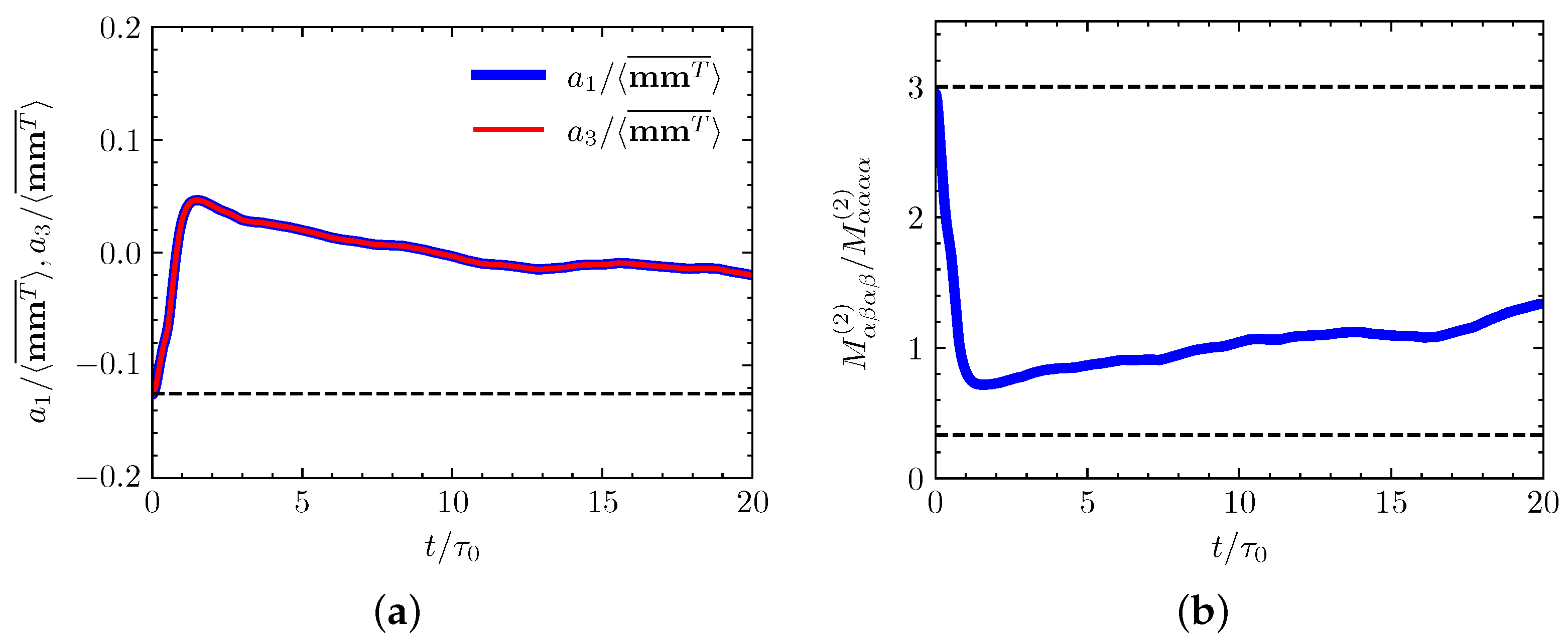
Figure 3.
(a) Time evolution of third-order invariants and , normalized by , which should be equal in 2D isotropic compressible turbulence. (b) Time evolution of third-order independent components and , normalized by , which should be equal in strictly isotropic 2D compressible turbulence.
Figure 3.
(a) Time evolution of third-order invariants and , normalized by , which should be equal in 2D isotropic compressible turbulence. (b) Time evolution of third-order independent components and , normalized by , which should be equal in strictly isotropic 2D compressible turbulence.

Table 1.
All non-zero types of . The subscripts in the type name only show different numbers without applying the Einstein summation convention.
Table 1.
All non-zero types of . The subscripts in the type name only show different numbers without applying the Einstein summation convention.
| Type | Examples | Expression with Independent Scalar |
|---|---|---|
Table 2.
All non-zero types of . The subscripts in the type name only show different numbers without applying the Einstein summation convention. The order of three pairs, i.e., , could be interchanged symmetrically.
Table 2.
All non-zero types of . The subscripts in the type name only show different numbers without applying the Einstein summation convention. The order of three pairs, i.e., , could be interchanged symmetrically.
| Type | Examples | Expression with Independent Scalar |
|---|---|---|
| , etc. | ||
| and | , etc. | |
| , etc. |
Table 3.
Second-order invariants of the velocity gradient under the isotropic constraints.
| Tensor Notation | Subscript Notation | Expression of and | Independent Scalar Expression |
|---|---|---|---|
Table 4.
Third-order invariants of the velocity gradient under the isotropic constraints.
| Tensor Notation | Subscript Notation | Expression of and | Independent Scalar Expression |
|---|---|---|---|
Disclaimer/Publisher’s Note: The statements, opinions and data contained in all publications are solely those of the individual author(s) and contributor(s) and not of MDPI and/or the editor(s). MDPI and/or the editor(s) disclaim responsibility for any injury to people or property resulting from any ideas, methods, instructions or products referred to in the content. |
© 2024 by the authors. Licensee MDPI, Basel, Switzerland. This article is an open access article distributed under the terms and conditions of the Creative Commons Attribution (CC BY) license (https://creativecommons.org/licenses/by/4.0/).
Share and Cite
MDPI and ACS Style
Luo, C.; Yang, P.-F.; Fang, L. Low-Order Moments of Velocity Gradient Tensors in Two-Dimensional Isotropic Turbulence. Symmetry 2024, 16, 175. https://doi.org/10.3390/sym16020175
AMA Style
Luo C, Yang P-F, Fang L. Low-Order Moments of Velocity Gradient Tensors in Two-Dimensional Isotropic Turbulence. Symmetry. 2024; 16(2):175. https://doi.org/10.3390/sym16020175
Chicago/Turabian StyleLuo, Chensheng, Ping-Fan Yang, and Le Fang. 2024. "Low-Order Moments of Velocity Gradient Tensors in Two-Dimensional Isotropic Turbulence" Symmetry 16, no. 2: 175. https://doi.org/10.3390/sym16020175
Note that from the first issue of 2016, this journal uses article numbers instead of page numbers. See further details here.