
Solitary Solutions for the Stochastic Fokas System Found in Monomode Optical Fibers


1
Department of Mathematics, College of Science, University of Ha’il, P.O.~Box 2440, Ha’il 81451, Saudi Arabia
2
Department of Mathematics, Faculty of Science, Mansoura University, Mansoura 35516, Egypt
3
Department of Mathematical Science, College of Science, Princess Nourah Bint Abdulrahman University, P.O. Box 84428, Riyadh 11671, Saudi Arabia
4
Section of Mathematics, International Telematic University Uninettuno, Corso Vittorio Emanuele II, 39, 00186 Roma, Italy
*
Author to whom correspondence should be addressed.
Symmetry 2023, 15(7), 1433; https://doi.org/10.3390/sym15071433
Submission received: 20 June 2023
/
Revised: 11 July 2023
/
Accepted: 14 July 2023
/
Published: 17 July 2023
(This article belongs to the Special Issue Recent Advances in Symmetries Methods and Other Approaches to Nonlinear Differential Equations)
Abstract
:The stochastic Fokas system (SFS), driven by multiplicative noise in the Itô sense, was investigated in this study. Novel trigonometric, rational, hyperbolic, and elliptic stochastic solutions are found using a modified mapping method. Because the Fokas system is used to explain nonlinear pulse propagation in monomode optical fibers, the solutions provided may be utilized to analyze a broad range of critical physical phenomena. In order to explain the impacts of multiplicative noise, the dynamic performances of the different found solutions are illustrated using 3D and 2D curves. We conclude that multiplicative noise eliminates the symmetry of the solutions of the SFS and stabilizes them.
MSC:
35A20; 60H10; 60H15; 35Q51; 83C151. Introduction
Nonlinear evolution equations (NLEEs) play an essential part in the comprehension of numerous significant phenomena and dynamic processes in engineering technology science, life science, geoscience, mechanics, and physics due to the development of nonlinear science. It is crucial to investigate the exact explicit solutions of NLEEs in order to gain a deeper understanding of the phenomena described by NLEEs. In recent years, quite a few techniques, including the first-integral method [1], sine–cosine procedure [2], exp-function method [3], Jacobi elliptic function expansion [4], mapping method [5], auxiliary equation scheme [6], extended tanh function method [7], generalized Kudryashov approach [8], -expansion method [9], F-expansion approach [10], Taylor’s power series expansion [11], q-homotopy analysis transform method [12], bifurcation analysis [13,14], and -expansion [15,16], have been proposed for solving NLEEs. Moreover, the Lie symmetry method [17] is the most significant method for developing analytical solutions for nonlinear NLEEs.
Until the 1950s, deterministic models of differential equations played an important role in the study of natural phenomena across a vast array of physical sciences. Nevertheless, it is evident that the phenomena that occur in the world today are not deterministic in nature. For these NLEEs, it is crucial to take random effects into account. Equations that take into account random fluctuations are called stochastic NLEEs. These kinds of equations are increasingly being utilized in the climate, biophysics, condensed matter, electrical engineering, information systems, finance, materials sciences, and other disciplines to develop mathematical models of complex processes [18,19]. In recent years, analytical solutions for some stochastic NLEEs, for example [20,21,22], have been discovered.
In this paper, we consider the Fokas system, which is one of the most significant of the NLEEs, forced by multiplicative noise:
where and are complex functions, and are arbitrary constants, is the noise strength. is the Brownian motion, . If we set , then we have the deterministic Fokas system (DFS):
Fokas [23] and Shulman [24] introduced the DFS (2) for examining NLSE in (2 + 1) dimensions. Because of the crucial role of DFS (2), numerous authors have attained the exact solutions by employing numerous techniques, such as the exp-function method [25], Jacobi elliptic function expansion [26], He’s frequency formulation method, the extended rational sinh–cosh and sine–cosine [27], the variational method and simplified extended tanh-function [28], Hirota’s bilinear method [29], and the generalized Kudryashov method [30]. The stochastic Fokas system (SFS) (1) has not been studied until now.
The objective of this study is to acquire the analytical stochastic solutions of the SFS (1). We use a modified mapping method to obtain the stochastic solutions of SFS (1) in the form of rational, elliptic, hyperbolic, and trigonometric functions. Since the Fokas system is used to explain nonlinear pulse propagation in monomode optical fibers, the obtained solutions can be applied to the analysis of a wide variety of crucial physical phenomena. The dynamic performances of the various obtained solutions are depicted using 3D and 2D curves in order to interpret the effects of multiplicative noise.
The paper has the following structure: In the next section, we derive the wave equation for the SFS (1). In Section 3, the modified mapping technique is employed to derive the exact solutions of SFS (1). In Section 4, we analyze the impact of the Brownian motion on the solution of SFS (1). Finally, the conclusion of the paper is provided.
2. Traveling Wave Equation for SFS
We utilize
to obtain the wave equation for SFS (1), where is a deterministic and real function, and are non-zero constants. We note that
where is the Itô correction term, and
Plugging Equations (4) and (5) into Equation (1), for the real part, we have
and for the imaginary part:
Setting that
3. Exact Solutions of SFS
Here, the modified mapping method described in [31] is applied. Let the solutions of Equation (13) have the following form:
where and are undetermined constants to be calculated, and u solves
where , and are real constants.
With , Equation (15) has the form
For we balance each coefficient of and with 0 to have
and
We obtain three distinct sets when we solve these equations:
First set:
Second set:
Third set:
Many cases rely on
Many cases rely on
Many cases rely on and
Case 3-2: If and then Thus, using Equations (81) and (82), the solutions of SFS (1) are
where When Equation (87) tends to
Case 3-3: If and then Thus, using Equations (81) and (82), the solutions of SFS (1) are
where When Equation (91) tends to
4. Impacts of Noise
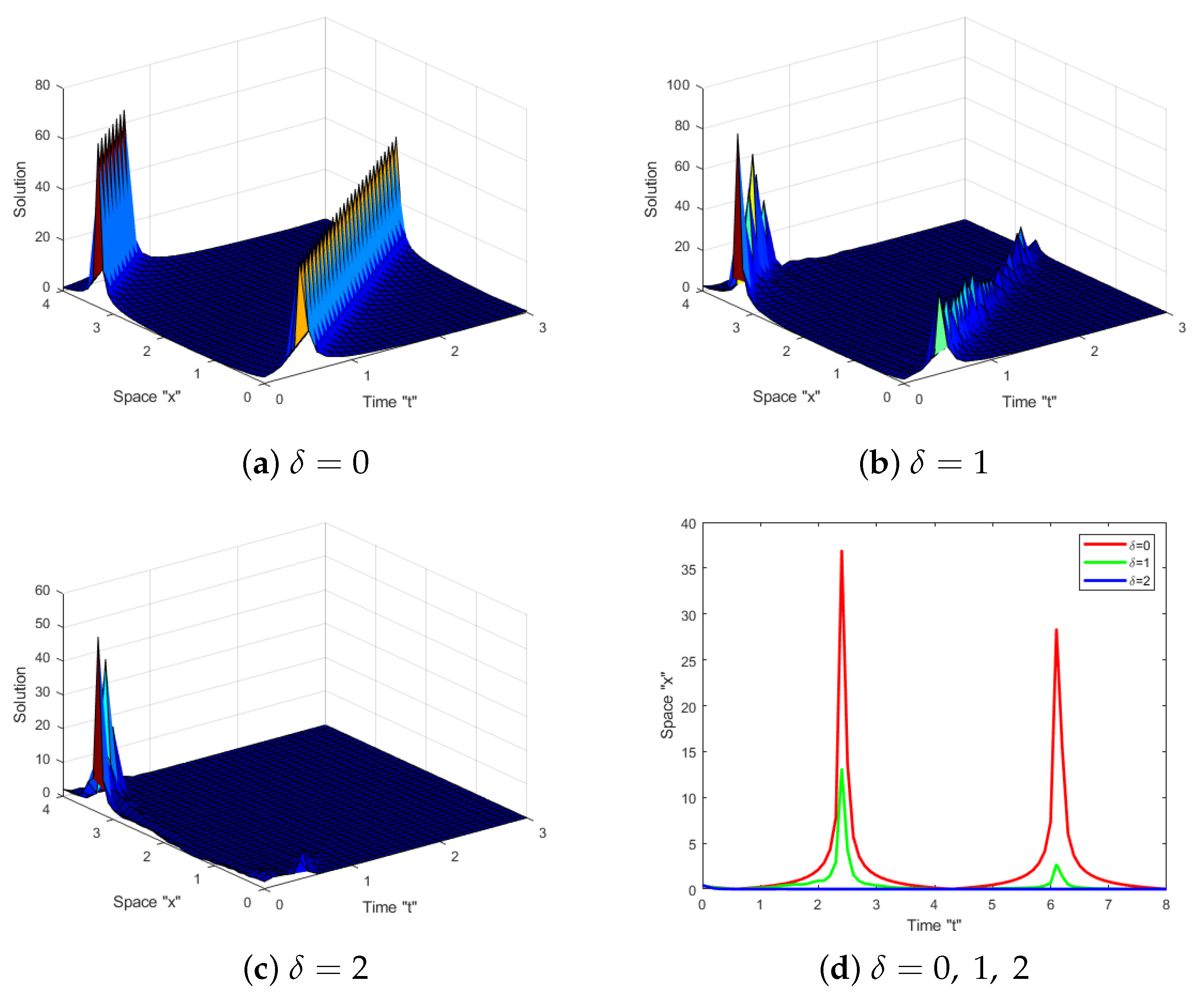
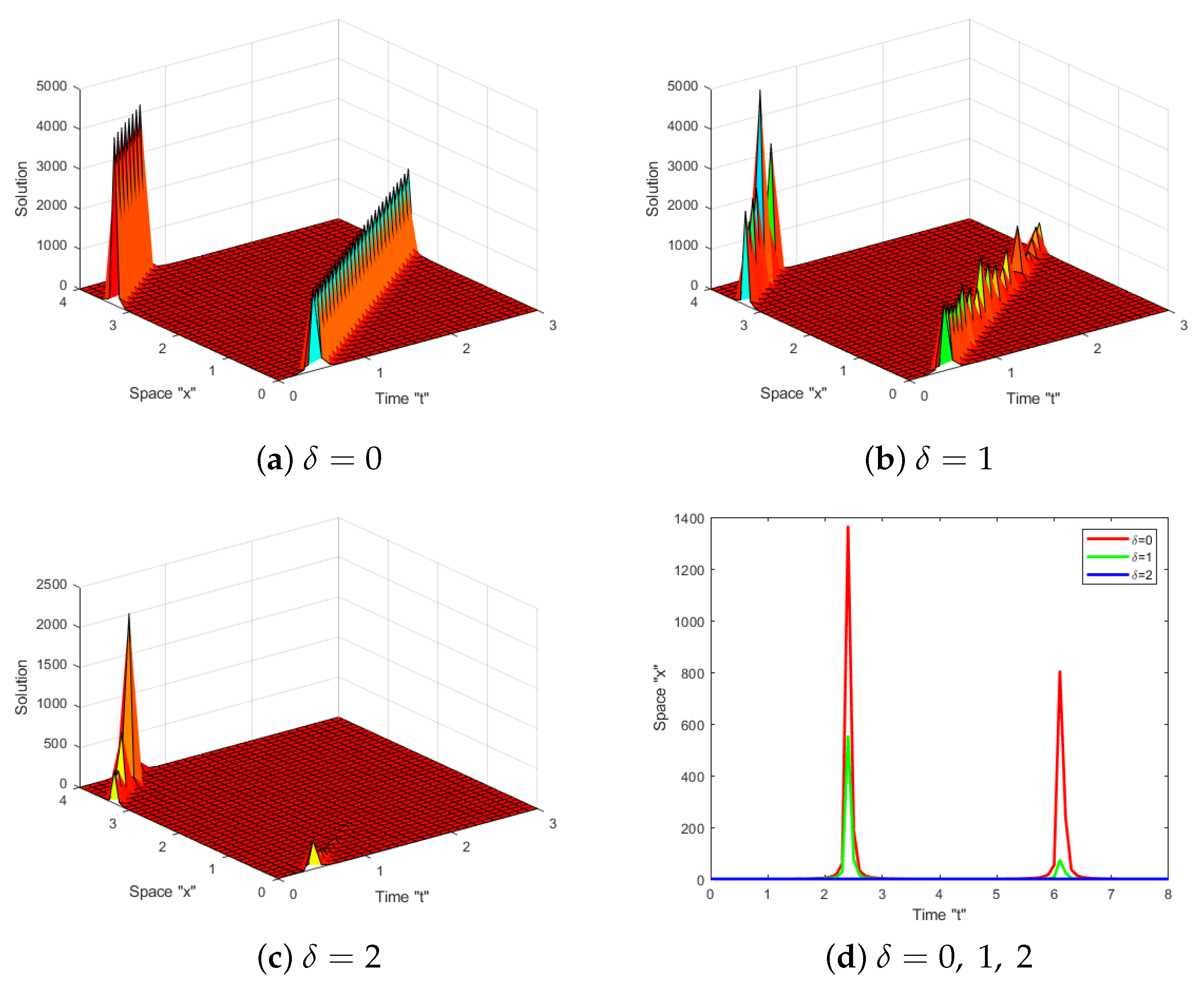
In this section, we address the effect of Brownian motion on the exact solution of the SFS (1). Several diagrams are supplied to show the behaviors of some obtained solutions, such as (23)–(26), (47) and (48). Let us fix the parameters and to simulate these diagrams.
Now, we can see from Figure 1, Figure 2, Figure 3, Figure 4, Figure 5 and Figure 6 that when the Brownian motion is ignored (i.e., when ), there are many other kinds of solutions, including periodic solutions, kink solutions, and so on. After short transit patterns, the surface becomes flatter when noise is incorporated and its amplitude is increased by . This demonstrates that Brownian motion stabilizes the SFS solutions, maintaining them around zero.
5. Conclusions
In this work, we considered the stochastic Fokas system (SFS) perturbed by multiplicative Brownian motion in the Itô sense. Utilizing a modified mapping method, we obtained the exact stochastic solutions. Due to the implementation of the Fokas system in explaining nonlinear pulse propagation in monomode optical fibers, these solutions can explain a wide array of fascinating and intricate physical phenomena. Using 3D and 2D curves for various values of noise strength, we depicted the dynamic behaviors of the numerous obtained solutions in order to interpret the effects of Brownian motion on these solutions. Furthermore, we established that multiplicative noise stabilizes the solutions at zero.
Author Contributions
Data curation, F.M.A.-A. and W.W.M.; formal analysis, W.W.M., F.M.A.-A. and C.C.; funding acquisition, F.M.A.-A.; methodology, C.C.; project administration, W.W.M.; software, W.W.M.; supervision, C.C.; visualization, F.M.A.-A.; writing—original draft, F.M.A.-A.; writing—review and editing, W.W.M. and C.C. All authors have read and agreed to the published version of the manuscript.
Funding
This research received no external funding.
Data Availability Statement
Not applicable.
Acknowledgments
Princess Nourah bint Abdulrahman University Researcher Supporting Project number (PNURSP2023R 273), Princess Nourah bint Abdulrahman University, Riyadh, Saudi Arabia.
Conflicts of Interest
The authors declare no conflict of interest.
References
- Lu, B. The first integral method for some time fractional differential equations. J. Math Anal. Appl. 2012, 395, 684–693. [Google Scholar] [CrossRef] [Green Version]
- Wazwaz, A.M. The sine-cosine method for obtaining solutions with compact and noncompact structures. Appl. Math. Comput. 2004, 159, 559–576. [Google Scholar] [CrossRef]
- He, J.H.; Wu, X.H. Exp-function method for nonlinear wave equations. Chaos Solitons Fractals 2006, 30, 700–708. [Google Scholar] [CrossRef]
- Yan, Z.L. Abunbant families of Jacobi elliptic function solutions of the dimensional integrable Davey-Stewartson-type equation via a new method. Chaos Solitons Fractals 2003, 18, 299–309. [Google Scholar] [CrossRef]
- Mohammed, W.W.; Al-Askar, F.M.; Cesarano, C. The Analytical Solutions of the Stochastic mKdV Equation via the Mapping Method. Mathematics 2022, 10, 4212. [Google Scholar] [CrossRef]
- Jiong, S. Auxiliary equation method for solving nonlinear partial differential equations. Phys. Lett. A 2003, 309, 387–396. [Google Scholar]
- Al-Askar, F.M.; Cesarano, C.; Mohammed, W.W. Abundant Solitary Wave Solutions for the Boiti-Leon-Manna-Pempinelli Equation with M-Truncated Derivative. Axioms 2023, 12, 466. [Google Scholar] [CrossRef]
- Arnous, A.H.; Mirzazadeh, M. Application of the generalized Kudryashov method to Eckhaus equation. Nonlinear Anal Model. Control. 2016, 21, 577–586. [Google Scholar] [CrossRef] [Green Version]
- Khan, K.; Akbar, M.A. The exp(-ϕ(ς))-expansion method for finding travelling wave solutions of Vakhnenko-Parkes equation. Int. J. Dyn. Syst. Differ. Equ. 2014, 5, 72–83. [Google Scholar]
- Al-Askar, F.M.; Cesarano, C.; Mohammed, W.W. The Influence of White Noise and the Beta Derivative on the Solutions of the BBM Equation. Axioms 2023, 12, 447. [Google Scholar] [CrossRef]
- Preethi, G.T.; Magesh, N.; Gatti, N.B. An Application of Conformable Fractional Differential Transform Method for Smoking Epidemic Model. Math. Comput. 2022, 415, 399–411. [Google Scholar]
- Veeresha, P.; Prakasha, D.G.; Magesh, N.; Christopher, A.J.; Sarwe, D.U. Solution for fractional potential KdV and Benjamin equations using the novel technique. J. Ocean Eng. Sci. 2021, 6, 265–275. [Google Scholar] [CrossRef]
- Elmandouh, A.; Fadhal, E. Bifurcation of Exact Solutions for the Space-Fractional Stochastic Modified Benjamin-Bona-Mahony Equation. Fractal Fract. 2022, 6, 718. [Google Scholar] [CrossRef]
- Alhamud, M.; Elbrolosy, M.; Elmandouh, A. New Analytical Solutions for Time-Fractional Stochastic (3 + 1)-Dimensional Equations for Fluids with Gas Bubbles and Hydrodynamics. Fractal Fract. 2023, 7, 16. [Google Scholar] [CrossRef]
- Wang, M.L.; Li, X.Z.; Zhang, J.L. The (G′/G)-expansion method and travelling wave solutions of nonlinear evolution equations in mathematical physics. Phys. Lett. A 2008, 372, 417–423. [Google Scholar] [CrossRef]
- Zhang, H. New application of the (G′/G)-expansion method. Commun. Nonlinear Sci. Numer. Simul. 2009, 14, 3220–3225. [Google Scholar] [CrossRef]
- Hydon, P.E. Symmetry Methode for differential Aquations; Cambridge University Press: Cambridge, UK, 2002. [Google Scholar]
- Arnold, L. Random Dynamical Systems; Springer: New York, NY, USA, 1998. [Google Scholar]
- Imkeller, P.; Monahan, A.H. Conceptual stochastic climate models. Stoch. Dyn. 2002, 2, 311–326. [Google Scholar] [CrossRef] [Green Version]
- Al-Askar, F.M.; Cesarano, C.; Mohammed, W.W. The Solitary Solutions for the Stochastic JimboMiwa Equation Perturbed by White Noise. Symmetry 2023, 15, 1153. [Google Scholar] [CrossRef]
- Al-Askar, F.M.; Cesarano, C.; Mohammed, W.W. Multiplicative Brownian Motion Stabilizes the Exact Stochastic Solutions of the Davey–Stewartson Equations. Symmetry 2022, 14, 2176. [Google Scholar] [CrossRef]
- Mohammed, W.W.; Cesarano, C. The soliton solutions for the (4 + 1)-dimensional stochastic Fokas equation. Math. Methods Appl. Sci. 2023, 46, 7589–7597. [Google Scholar] [CrossRef]
- Fokas, A.S. On the simplest integrable equation in 2 + 1. Inverse Probl. 1994, 10, L19. [Google Scholar] [CrossRef] [Green Version]
- Shulman, E.I. On the integrability of equations of Davey Stewartson type. Teor. Mat. Fiz. 1983, 56, 131–136. [Google Scholar] [CrossRef]
- Wang, K.J. Abundant exact soliton solutions to the Fokas system. Optik 2022, 249, 168265. [Google Scholar] [CrossRef]
- Tarla, S.; Ali, K.K.; Sun, T.C.; Yilmazer, R.; Osman, M.S. Nonlinear pulse propagation for novel optical solitons modeled by Fokas system in monomode optical fibers. Results Phys. 2022, 36, 1053. [Google Scholar] [CrossRef]
- Wang, K.J.; Liu, J.H.; Wu, J. Soliton solutions to the Fokas system arising in monomode optical fibers. Optik 2022, 251, 168319. [Google Scholar] [CrossRef]
- Zhang, P.L.; Wang, K.J. Abundant optical soliton structures to the Fokas system arising in monomode optical fibers. Open Phys. 2022, 20, 493–506. [Google Scholar] [CrossRef]
- Rao, J.; Mihalache, D.; Cheng, Y.; He, J. Lump-soliton solutions to the Fokas system. Phys. Lett. A 2019, 383, 1138–1142. [Google Scholar] [CrossRef]
- Kaplan, M.; Akbulut, A.; Alqahtani, R.T. New Solitary Wave Patterns of the Fokas System in Fiber Optics. Mathematics 2023, 11, 1810. [Google Scholar] [CrossRef]
- Bhrawy, A.H.; Abdelkawy, M.A.; Kumar, S.; Johnson, S.; Biswas, A. Solitons and other solutions to quantum Zakharov–Kuznetsov equation in quantum magneto-plasmas. Indian J. Phys. 2013, 87, 455–463. [Google Scholar] [CrossRef]
Figure 1.
(a–c) The 3D style of solution in Equation (23) with and ; (d) the 2D style of Equation (23) with different values of .

Figure 2.
(a–c) The 3D style of solution in Equation (24) with and ; (d) the 2D style of Equation (24) with different values of .
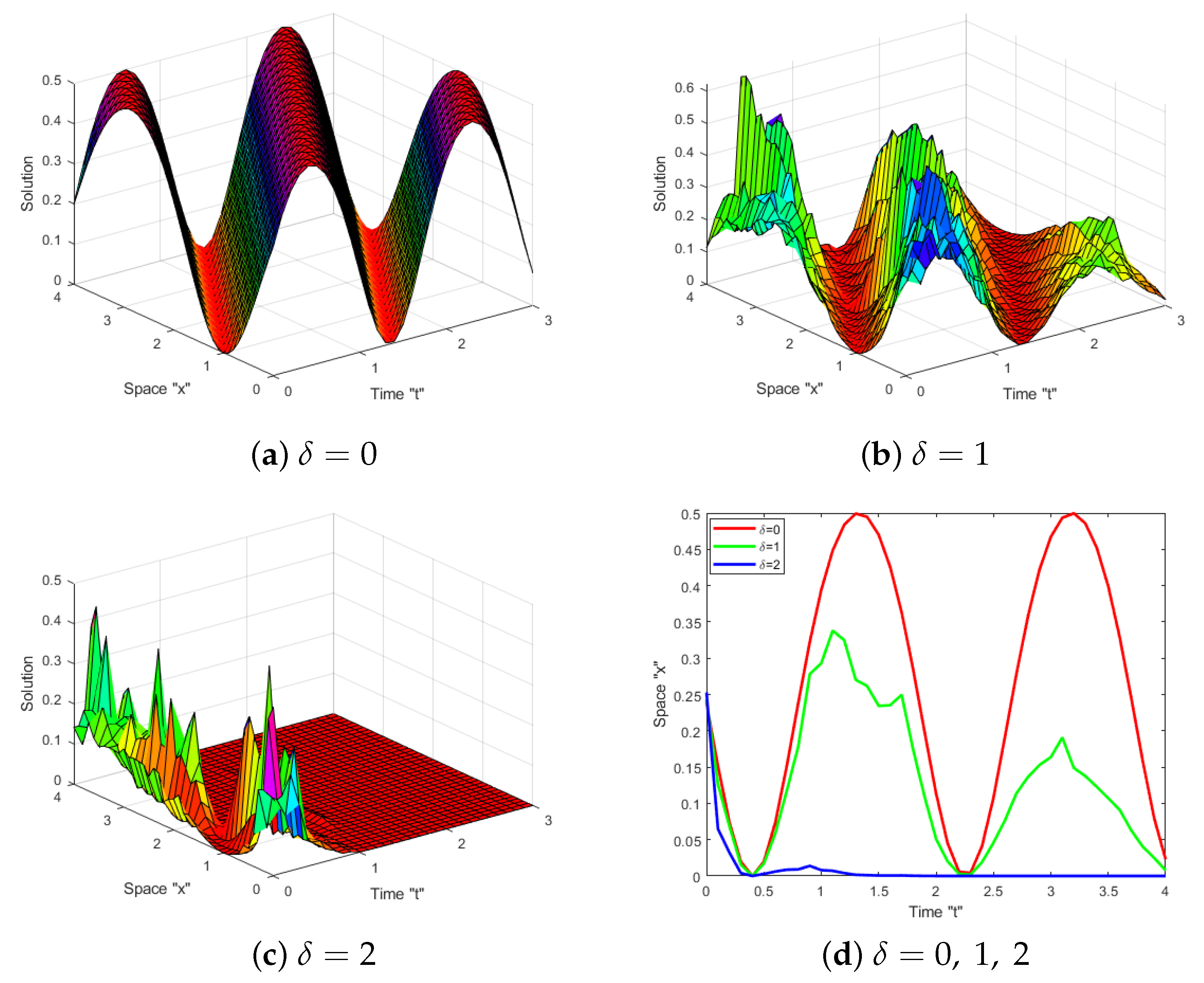
Figure 3.
(a–c) The 3D style of solution in Equation (25) with and ; (d) the 2D style of Equation (25) with different values of .

Figure 4.
(a–c) The 3D style of solution in Equation (26) with and ; (d) the 2D style of Equation (26) with different values of .
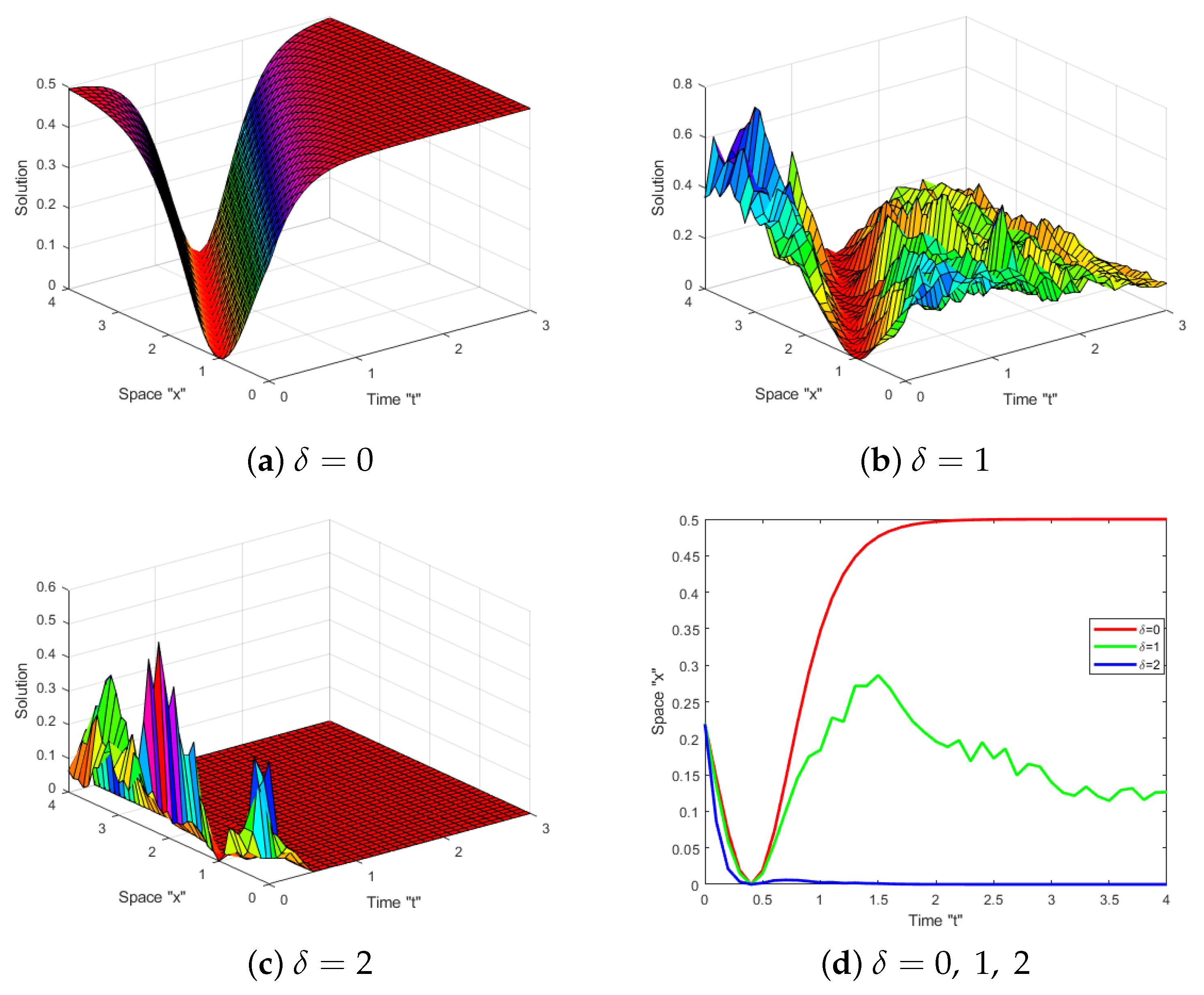
Figure 5.
(a–c) The 3D style of solution in Equation (47) with and ; (d) the 2D style of Equation (23) with different values of .
Disclaimer/Publisher’s Note: The statements, opinions and data contained in all publications are solely those of the individual author(s) and contributor(s) and not of MDPI and/or the editor(s). MDPI and/or the editor(s) disclaim responsibility for any injury to people or property resulting from any ideas, methods, instructions or products referred to in the content. |
© 2023 by the authors. Licensee MDPI, Basel, Switzerland. This article is an open access article distributed under the terms and conditions of the Creative Commons Attribution (CC BY) license (https://creativecommons.org/licenses/by/4.0/).
Share and Cite
MDPI and ACS Style
Mohammed, W.W.; Al-Askar, F.M.; Cesarano, C. Solitary Solutions for the Stochastic Fokas System Found in Monomode Optical Fibers. Symmetry 2023, 15, 1433. https://doi.org/10.3390/sym15071433
AMA Style
Mohammed WW, Al-Askar FM, Cesarano C. Solitary Solutions for the Stochastic Fokas System Found in Monomode Optical Fibers. Symmetry. 2023; 15(7):1433. https://doi.org/10.3390/sym15071433
Chicago/Turabian StyleMohammed, Wael W., Farah M. Al-Askar, and Clemente Cesarano. 2023. "Solitary Solutions for the Stochastic Fokas System Found in Monomode Optical Fibers" Symmetry 15, no. 7: 1433. https://doi.org/10.3390/sym15071433
Note that from the first issue of 2016, this journal uses article numbers instead of page numbers. See further details here.