
Statistical Analyses of a Class of Random Cyclooctatetraene Chain Networks with Respect to Several Topological Properties
School of Mathematics and Big Data, Anhui University of Science & Technology, Huainan 232001, China
*
Author to whom correspondence should be addressed.
Symmetry 2023, 15(11), 1971; https://doi.org/10.3390/sym15111971
Submission received: 19 September 2023
/
Revised: 17 October 2023
/
Accepted: 20 October 2023
/
Published: 24 October 2023
(This article belongs to the Special Issue Symmetry and Graph Theory)
Abstract
:In recent years, the research on complex networks has created a boom. The objective of the present paper is to study a random cyclooctatetraene chain whose graph-theoretic mathematical properties arose scientists’ interests. By applying the concept of symmetry and probability theory, we obtain the explicit analytical expressions for the variances of Schultz index, multiplicative degree-Kirchhoff index Gutman index, and additive degree-Kirchhoff index of a random cyclooctatetraene chain with n octagons, which plays a crucial role in the research and application of topological indices.
1. Introduction
In this paper, we just take finite and simple connected graphs into consideration, referring to [1] and the references cited therein. Chemistry is strongly linked to graph theory, and graph theory has been widely used in chemistry. In chemical graph theory, there are some alternatives between atoms that vertices represent the atoms and edges represent the covalent bonds. They are used to depict chemical compounds.
The molecular formula of a compound can represent different molecular structures and characteristics, but theoretical chemists are concerned with the physical and chemical properties of a compound and its relationship with the molecular formula of a compound. The physical and chemical properties of compounds are key areas of concern for theoretical chemists [2,3]. Polygonal chemicals have a wide diversity of molecular structures and their physical and chemical properties are becoming increasingly significant, which is referenced in [4,5,6,7].
There is no octagon in octagonal chains that has more than two cut-vertices, and such a octagonal chain is called a cyclooctatetraene chain. Cyclooctatetraene is the poster child for nonaromatic molecules. Cyclooctatetraene and its derivatives have fascinated chemists for a long time and have a wide range of applications in industry. Cyclooctatetraene differs from benzene in that it is not an aromatic hydrocarbon. It is chemically close to an unsaturated hydrocarbon. Not only can it be subjected to addition reactions, which is easily hydrogenated to form cyclooctane. It also oxidises and polymerises readily. A number of vital compounds of cyclooctatetraene can be served as substrates for the production of scientifically and commercially valuable materials. In this paper, we consider four kinds of indices of cyclooctatetraene chains with n octagons. We simply consider the situation starting from a vertex of a cyclooctatetraene chain, connecting an edge to another octagon. For more information about the cyclooctylene chain, we can refer to [8,9,10,11].
We give some basic notations. Set be a graph with vertices denoted and edges denoted . The number of edges in a graph G is denoted by . We claim that two vertices p and m are adjacent (or neighbours) if they are attached by an edge, which we will write as . In G, the shortest length -path among the paths between two vertices p and m is denoted as (or simply ). The Wiener index of G refers to the aggregate of distances between all the vertex pairs of G. It was created by H. Wiener in 1947 [12], that is
The Wiener index is among the best studied, most understood, and most widely used molecular shape descriptors, and is based on graph theory, see [13,14,15,16].
A graph together with the weight function : is known as a weighted graph [17] . Let ⊕ denote one of the four arithmetic operations [18]. Consequently, the weighted Wiener index is determined as
Obviously, if and ⊕ denotes the operation ×, then .
In case ⊕ represents the operation × and , then (2) is equivalent to [19]
This is just the Gutman index. Research on possible chemical applications of the Gutman index and similar quantities and their theoretical study, for which polycyclic molecules are more difficult cases, see [20].
In case ⊕ represents the operation + and , then (2) is equivalent to
That’s what the Schultz Index is all about. For additional articles on developing aspects of the topology indexes for [21,22,23,24], including mathematical properties, discrimination and applications, refer to [25].
In case of , the resistance distance between a and b in G, is defined as the effective resistance between nodes a and b in the electrical network, where the nodes correspond to vertices of G and each edge of G is replaced by a resistor of unit resistance. The resistance distance between vertices a and b in G [26] is denoted as . For more detailed information, see [27,28,29,30]. It is the Kirchhoff index when the Wiener index is for non-trees, and this distance function is proposed by Klein and Randić [31], defined as
For a description of the sum of eccentricity distances and the sum of eccentricity resistance-distances, refer to [32,33,34,35,36].
Thus, the invariance of this graph is represented as
from which are the eigenvalues of . Moreover, is the normalized Laplacian matrix of G, as proposed by Chung [39]. The normalized Laplacian index and multiplicative degree-Kirchhoff index play an essential application in mathematical chemistry and statistics. Research on these topics has attracted a wide range of attention from researchers.
was introduced by Gutman, Feng and Yu in 2012 [40], which is defined as
Probability properties are an important component of chemical graphs, which can more broadly describe the topological properties and structures of chemical graphs. In this paper, we focus on the cyclooctatetraene chain with n octagons, which is formed as follows.
Firstly, is an octagon and is the graph with two octagons, as shown in Figure 1.
Secondly, by appending a new terminal octagon to , the random cyclooctatetraene chain with n octagons can be constructed. We illustrates this process in Figure 2. As demonstrated in Figure 3, we can append the terminal octagon to with four methods and indicate the generated figures with , , , and , respectively.
At each step, randomly pick one of the following possible outcomes:
- is the probability that ;
- is the probability that
- is the probability that
- is the probability that .
We consider four random variables , , , and for our choice. When , in case our selection is , we have ; otherwise, , and we can easily derive that
and .
Through the above process, we get a random cyclooctatetraene chain . We always abbreviate to . All of , , and are random variables in probability by noting that is a random graph. From a probabilistic point of view, a natural question arises: when n is big enough, will the distribution of , , and look like a probability distribution or not.
In this paper, we make researches on , , and . There is a huge amount of relevant literature. For random polyphenylene chain, J.I. Zhang, X.H. Peng, H.I. Chen [18] established the limiting behaviours of , , and . Here it is natural and interesting to consider limiting behaviours of , , and for random cyclooctatetraene chain. In this paper, by applying the concept of symmetry and probability theory, we derive definite analytical expressions for the variance of the Schultz index, multiplicative degree-Kirchhoff index, Gutman index and additive degree-Kirchhoff index of a random cyclooctatetraene chain with n octagons, which plays a crucial role in the research and application of topological indices.
In this paper, in order to better describe the probability properties of cyclooctylene chain, we propose the following hypothesis.
Hypothesis 1.
We choose to attach the new terminal octagon to , where , and it is random and independent. More precisely, a range of random variables is independent and has the same law (9). With regard to some , is obvious. Based on Hypothesis 1, we present analytical expressions for the variances of , , and .
2. The Variances for the Gutman Index and Schultz Index of a Random Cyclooctatetraene Chain
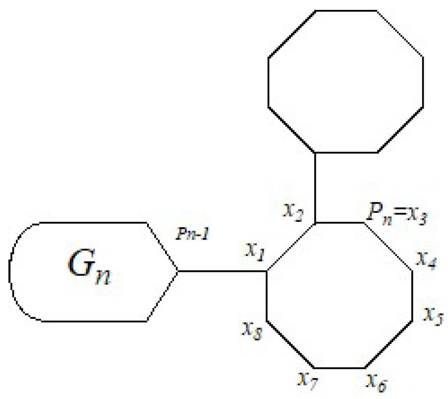
For all , the Gutman index and Schultz index of a random cyclooctatetraene chain are random variables. We are going to take the variances of and into consideration in this section. Actually, is connected by an edge to a new terminal octagon , where is extended by vertices , , , , , , , and , and is the new edge; see Figure 2. On the one hand, for all ,
on the other hand, for all
In [41] Theorem 1, the author proves that
where is the mathematical expectations of .
We now present the first main result of this section.
Theorem 1.
The results are as follows, if Hypothesis 1 holds. As to the random cyclooctatetraene chain , the variance of Gutman index , computed as
where
Proof.
Recalling from Section 1 that , , , and are random variables, this indicates our option in constructing from . We have four equalities as follows:
Equality 1.
If , the equality mentioned above is evident. Thus, we only have to regard the case , which means that . In this view, (of ) is coincident with the vertex labeled or (of ), see Figure 4. In this scenario, turns into
In the foregoing, we utilised (10)–(12). As a result, we arrive at the required equivalence conclusion.
Equality 2.
As in the proof of Equality 1, we only have to regard the case , which is . The proof process is analogous, and we leave out the details.
Equality 3.
We have to regard the case , which is . The proof is the same as Equality 1 and we omit the details.
Equality 4.
We have to regard the case , which is . The proof process is also analogous, and we leave out the details.
Recalling that , according to the above discussion, it holds that
For each n, it indicates that , .
Therefore, by (15) we obtain
where representing high-order infinitesimal of .
By direct calculation, one sees that , , and , where for any two random variables X and Y, . Based on the nature of the variance and the order in which the sums are exchanged, it can be concluded that
By means of computational, ad hoc tools, the above equality gives the required results, .
Now, we discuss the variance of the Schultz index.
By Theorem 2.3 of [41], we have
After that we illustrate our results.
Theorem 2.
Supposing that Hypothesis 1, then the following results are true. As to the random cyclooctatetraene chain , the variance of Schultz index , computed as
where
Proof.
After similar discussions, we have four equalities as follows:
Equality 1.
If , the equality mentioned above is evident, so we only have to regard the case , which means that . In this view, (of ) is coincident with the vertex labeled or (of ), see Figure 4. In this scenario, turns into
In the foregoing, we utilised (10)–(12). As a result, we arrive at the required equivalence conclusion.
Equality 2.
As in the proof of Equality 1, we only have to regard the case , which is . The proof process is analogous, and we leave out the details.
Equality 3.
We have to regard the case , which is . The proof is the same as Equality 1 and we omit the details.
Equality 4.
We have to regard the case , which is . The proof process is also analogous, and we leave out the details.
Recalling that , according to the above discussion, it holds that
where for each n, , .
Therefore, by (15)
If we replace from the proof of Theorem 1 by , the rest of the proof of this theorem is the same as the proof of Theorem 1, and therefore the details are omitted.
3. The Variances of Multiplicative and Additive Degree-Kirchhoff Indices of a Random Cyclooctatetraene Chain
In the section, we talk about the variances for the multiplicative degree-Kirchhoff index and the additive degree-Kirchhoff index . For a random cyclooctatetraene chain , and are random variables.
Recall that is connected by an edge to a new terminal octagon , where is extended by vertices , , , , , , , and , and is the new edge; see Figure 2. On the one hand, for all ,
On the other hand, for all
By Theorem 3.1 of [41], we have
we now present the first main result of this section.
Theorem 3.
The results are as follows, if Hypothesis 1 holds. As to the random cyclooctatetraene chain , the variance of the multiplicative degree-Kirchhoff index , computed as
where
Proof.
Recalling from Section 1 that , , , and are random variables, this indicates our option in constructing from . We have four equalities as follows:
Equality 1.
If , the above equality is obvious, so we only need to consider the case , which implies . In this view, (of ) is coincident with the vertex labeled or (of ), see Figure 4. In this scenario, turns into
In the foregoing, we utilised (17)–(19). As a result, we arrive at the required equivalence conclusion.
Equality 2.
As in the proof of Equality 1, we only have to regard the case , which is . The proof process is analogous, and we leave out the details.
Equality 3.
We have to regard the case , which is . The proof is the same as Equality 1 and we omit the details.
Equality 4.
We have to regard the case , which is . The proof process is also analogous, and we leave out the details.
Recalling that , according to the above discussion, it holds that
where for each n, , .
Therefore, by (22)
Now, we consider . By Theorem 3.3 of [41] we have
is given by
Theorem 4.
where
Proof.
Recalling from Section 1 that , , , and are random variables, this indicates our option in constructing from . We have four equalities as follows:
Equality 1.
If , the equality mentioned above is evident, so we only have to regard the case , which means that . In this view, (of ) is coincident with the vertex labeled or (of ), see Figure 4. In this scenario, turns into
In the foregoing, we utilised (17)–(19). As a result, we arrive at the required equivalence conclusion.
Equality 2.
As in the proof of Equality 1, we only have to regard the case , which is . The proof process is analogous, and we leave out the details.
Equality 3.
We have to regard the case , which is . The proof is the same as Equality 1 and we omit the details.
Equality 4.
We have to regard the case , which is . The proof process is also analogous, and we leave out the details.
Recalling that , according to the above discussion, it holds that
where for each n, , .
Therefore, by (25)
If we replace with in the proof of Theorem 1, the rest of the proof of this theorem is the same as that in the proof of Theorem 1; we thus omit the details.
4. Concluding Remarks
In this paper, we obtain explicit analytical expressions for the variances of Schultz index, multiplicative degree-Kirchhoff index, Gutman index and additive degree-Kirchhoff index of a random cyclooctatetraene chain with n octagons. All of these results will contribute to the study of Schultz index, multiplicative degree-Kirchhoff index, Gutman index and additive degree-Kirchhoff index of graphs. With the continuous development and progress of science, more and more molecules are being discovered and created.
The polygonal chain problem in chemical graph theory has been extensively studied and discussed by researchers. For the variance of some certain indices of a random polygon chain that has n regular polygons, it is feasible to establish exact formulas.
Not only that, through these studies, we can hopefully obtain the variance of the n sided chain graph and some of their physicochemical properties in the near future.
Author Contributions
Conceptualization, C.T., S.T. and X.G.; methodology, C.T.; software, C.T.; validation, C.T. and X.G.; formal analysis, C.T.; investigation, C.T.; resources, S.T.; data curation, C.T.; writing—original draft preparation, C.T.; writing—review and editing, C.T.; visualization, S.T.; supervision, C.T.; project administration, C.T.; funding acquisition, X.G. All authors have read and agreed to the published version of the manuscript.
Funding
The research is partially supported by National Science Foundation of China (Grant No. 12171190) and Natural Science Foundation of Anhui Province (Grant No. 2008085MA01).
Data Availability Statement
Not applicable.
Acknowledgments
The authors are very grateful to the helpful comments and suggestions. The research is partially supported by National Science Foundation of China (Grant No. 12171190) and Natural Science Foundation of Anhui Province (Grant No. 2008085MA01).
Conflicts of Interest
The authors declare no conflict of interest.
References
- Bondy, J.A.; Murty, U.S.R. Graph Theory; Springer: New York, NY, USA, 2008. [Google Scholar]
- Haruo, H.; Index, T. A Newly Proposed Quantity Characterizing the Topological Nature of Structural Isomers of Saturated Hydrocarbons. J. Bull. Chem. Soc. Jpn. 2006, 44, 2332–2339. [Google Scholar]
- Estrada, E. Edge Adjacency Relationships and a Novel Topological Index Related to Molecular Volume. J. Chem. Inf. Comput. Sci. 1995, 35, 31–33. [Google Scholar] [CrossRef]
- Person, W.B.; Pimentel, G.C.; Pitzer, K.S. The Structure of Cyclooctatetraene. J. Am. Chem. Soc. 1952, 74, 3437–3438. [Google Scholar] [CrossRef]
- Cope, A.C.; Pike, R.M.; Polyolefins, C. Cyclooctatetraene Derivatives from Copolymerization and Side Chain Modification. J. Am. Chem. Soc. 1953, 75, 3220–3223. [Google Scholar] [CrossRef]
- Luthe, G.; Jacobus, J.A.; Robertson, L.W. Receptor interactions by polybrominated diphenyl ethers versus polychlorinated biphenyls: A theoretical structure-activity assessment. Environ. Toxicol. Pharm. 2008, 25, 202–210. [Google Scholar] [CrossRef] [PubMed]
- Mathews, F.S.; Lipscomb, W.N. The Structure of Silver Cyclooctatetraene Nitrate. J. Phys. Chem. 1959, 63, 845–850. [Google Scholar] [CrossRef]
- Garavelli, M.; Bernardi, F.; Cembran, A. Cyclooctatetraene Computational Photo- and Thermal Chemistry: A Reactivity Model for Conjugated Hydrocarbons. J. Am. Chem. Soc. 2002, 124, 13770–13789. [Google Scholar] [CrossRef]
- Lo, D.H.; Whitehead, M.A. Molecular geometry and bond energy. III. Cyclooctatetraene and related compounds. J. Am. Chem. Soc. 1969, 91, 238–242. [Google Scholar] [CrossRef]
- Schwamm, R.J.; Anker, M.D.; Lein, M. Reduction vs. Addition: The Reaction of an Aluminyl Anion with 1,3,5,7-Cyclooctatetraene. J. Chem. 2019, 58, 1489–1493. [Google Scholar]
- Milas, N.; Nolan, J., Jr.; Otto, P.H.L. Notes-Ozonization of Cyclooctatetraene. J. Org. Chem. 1958, 23, 624–625. [Google Scholar] [CrossRef]
- Wiener, H. Structrual determination of paraffin boiling points. J. Am. Chem. Soc. 1947, 69, 17–20. [Google Scholar] [CrossRef] [PubMed]
- Buckley, F.; Harary, F. Distance in Graphs; Addison-Wesley: Reading, UK, 1989. [Google Scholar]
- Chen, A.L.; Zhang, F.J. Wiener index and perfect matchings in random phenylene chains. MATCH Commun. Math. Comput. Chem. 2009, 61, 623–630. [Google Scholar]
- Entringer, R.C.; Jackson, D.E.; Snyder, D.A. Distance in graphs. Czechoslov. Math. J. 1976, 26, 283–296. [Google Scholar] [CrossRef]
- Zhou, Q.N.; Wang, L.G.; Lu, Y. Wiener index and Harary index on Hamilton-connected graphs with large minimum degree. Discrete Appl. Math. 2018, 247, 180–185. [Google Scholar] [CrossRef]
- Zhang, L.I.; Li, Q.S.; Li, S.C.; Zhang, M.J. The expected values for the Schultz index, Gutman index, multiplicative degree-Kirchhoff index and additive degree-Kirchhoff index of a random polyphenylene chain. J. Discret. Appl. Math. 2020, 282, 243–256. [Google Scholar] [CrossRef]
- Zhang, J.L.; Peng, X.H.; Chen, H.L. The limiting behaviours for the Gutman index, Schultz index, multiplicative degree-Kirchhoff index and additive degree-Kirchhoff index of a random polyphenylene chain. Discrete Appl. Math. 2021, 299, 62–73. [Google Scholar] [CrossRef]
- Ayache, A.; Alameri, A. Topological indices of the mk-graph. J. Assoc. Arab. Univ. Basic Appl. Sci. 2017, 24, 283–291. [Google Scholar]
- Gutman, I. Selected properties of the Schultz molecular topological index. J. Chem. Inf. Comput. Sci. 1994, 34, 1087–1089. [Google Scholar] [CrossRef]
- Chen, S. Modified Schultz index of zig-zag polyhex nanotubes. J. Comput. Theor. Nanosci. 2009, 6, 1499–1503. [Google Scholar] [CrossRef]
- Farahani, M.R. Hosoya, Schultz, modified Schultz polynomials and their topological indices of benzene molecules: First members of polycyclic aromatic hydrocarbons (PAHs). Int. J. Theor. Chem. 2013, 1, 9–16. [Google Scholar]
- Heydari, A. On the modified Schultz index of C4C8(S) nanotubes and nanotorus. Digest. J. Nanomater. Biostruct. 2010, 5, 51–56. [Google Scholar]
- Xiao, Z.; Chen, S. The modified Schultz index of armchair polyhex nanotubes. J. Comput. Theor. Nanosci. 2009, 6, 1109–1114. [Google Scholar] [CrossRef]
- Mukwembi, S.; Munyira, S. MunyiraDegree distance and minimum degree. Bull. Aust. Math. Soc. 2013, 87, 255–271. [Google Scholar] [CrossRef]
- Qi, X.L.; Zhou, B.; Du, Z.B. The Kirchhoff indices and the matching numbers of unicyclic graphs. J. Appl. Math. Comput. 2016, 289. [Google Scholar] [CrossRef]
- Georgakopoulos, A. Uniqueness of electrical currents in a network of finite total resistance. J. Lond. Math. Soc. 2010, 82, 256–272. [Google Scholar] [CrossRef]
- Huang, S.B.; Zhou, J.; Bu, C.J. Some results on Kirchhoff index and degree-Kirchhoff index. MATCH Commun. Math. Comput. Chem. 2016, 75, 207–222. [Google Scholar]
- Cinkir, Z. Deletion and contraction identities for the resistance calues and the Kirchhoff index. Int. J. Quantum Chem. 2011, 111, 4030–4041. [Google Scholar] [CrossRef]
- Gupta, S.; Singh, M.; Madan, A.K. Eccentric distance sum: A novel graph invariant for predicting biological and physical properties. J. Math. Anal. Appl. 2002, 275, 386–401. [Google Scholar] [CrossRef]
- Klein, D.J.; Randić, M. Resistance distance. J. Math. Chem. 1993, 12, 81–95. [Google Scholar] [CrossRef]
- He, F.G.; Zhu, Z.X. Cacti with maximum eccentricity resistance-distance sum. Discret. Appl. Math. 2017, 219, 117–125. [Google Scholar] [CrossRef]
- Huang, Z.W.; Xi, X.Z.; Yuan, S.L. Some further results on the eccentric distance sum. J. Math. Anal. Appl. 2019, 470, 145–158. [Google Scholar] [CrossRef]
- Li, S.C.; Wei, W. Some edge-grafting transformations on the eccentricity resistance-distance sum and their applications. Discret. Appl. Math. 2016, 211, 130–142. [Google Scholar] [CrossRef]
- Somodi, M. On the Ihara zeta function and resistance distance-based indices. Linear Algebra Appl. 2017, 513, 201–209. [Google Scholar] [CrossRef]
- Yang, Y.J.; Klein, D.J. A note on the Kirchhoff and additive degree-Kirchhoff indices of graphs. Z. Naturforsch. A 2015, 70, 459–463. [Google Scholar] [CrossRef]
- Chen, H.; Zhang, F. Resistance distance and the normalized Laplacian spectrum. Discret. Appl. Math. 2007, 155, 654–661. [Google Scholar] [CrossRef]
- Tang, M.; Priebe, C.E. Limit theorems for eigenvectors of the normalized Laplacian for random graphs. Ann. Statist. 2018, 46, 2360–2415. [Google Scholar] [CrossRef]
- Chung, F.R.K. Spectral Graph Theory; American Mathematical Society: Providence, RI, USA, 1997. [Google Scholar]
- Gutman, I.; Feng, L.; Yu, G. Degree resistance distance of unicyclic graphs. Trans. Comb. 2012, 1, 27–40. [Google Scholar]
- Qi, J.F.; Ni, J.B.; Geng, X.Y. The expected values for the Kirchhoff indices in the random cyclooctatetraene and spiro chains. J. Discret. Appl. Math. 2022, 321, 240–249. [Google Scholar] [CrossRef]
Figure 1.
Graph .
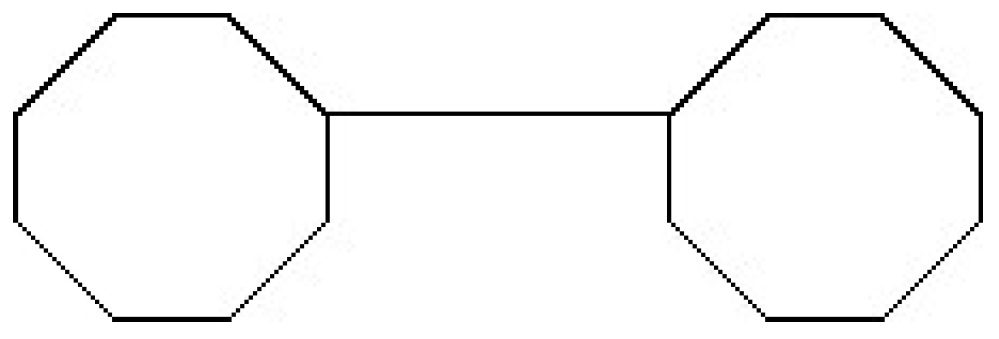
Figure 2.
The construction of from and .

Figure 3.
Four ways to attach the new terminal octagon to .
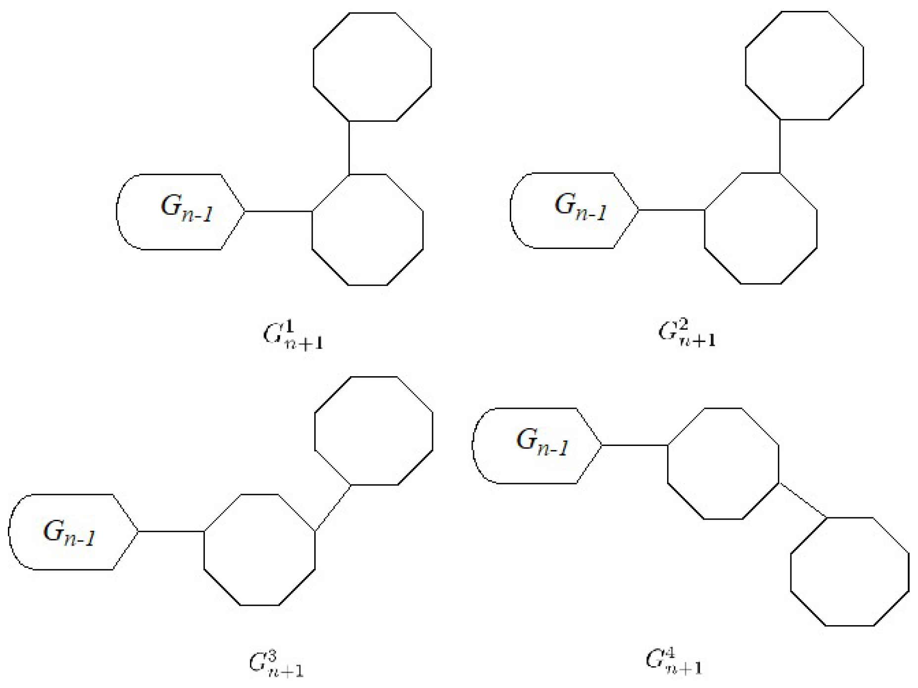
Figure 4.
.
Disclaimer/Publisher’s Note: The statements, opinions and data contained in all publications are solely those of the individual author(s) and contributor(s) and not of MDPI and/or the editor(s). MDPI and/or the editor(s) disclaim responsibility for any injury to people or property resulting from any ideas, methods, instructions or products referred to in the content. |
© 2023 by the authors. Licensee MDPI, Basel, Switzerland. This article is an open access article distributed under the terms and conditions of the Creative Commons Attribution (CC BY) license (https://creativecommons.org/licenses/by/4.0/).
Share and Cite
MDPI and ACS Style
Tao, C.; Tang, S.; Geng, X. Statistical Analyses of a Class of Random Cyclooctatetraene Chain Networks with Respect to Several Topological Properties. Symmetry 2023, 15, 1971. https://doi.org/10.3390/sym15111971
AMA Style
Tao C, Tang S, Geng X. Statistical Analyses of a Class of Random Cyclooctatetraene Chain Networks with Respect to Several Topological Properties. Symmetry. 2023; 15(11):1971. https://doi.org/10.3390/sym15111971
Chicago/Turabian StyleTao, Chen, Shengjun Tang, and Xianya Geng. 2023. "Statistical Analyses of a Class of Random Cyclooctatetraene Chain Networks with Respect to Several Topological Properties" Symmetry 15, no. 11: 1971. https://doi.org/10.3390/sym15111971
Note that from the first issue of 2016, this journal uses article numbers instead of page numbers. See further details here.