
On a Unique Solution of a Class of Stochastic Predator–Prey Models with Two-Choice Behavior of Predator Animals


1
Department of Mathematics, College of Science and Humanities in Al-Kharj, Prince Sattam Bin Abdulaziz University, Al-Kharj 11942, Saudi Arabia
2
Department of Mathematics and Computer Science, St. Thomas College, Bhilai 490006, India
3
Faculty of Electrical Engineering, University of Banja Luka, Patre 5, 78000 Banja Luka, Bosnia and Herzegovina
4
Department of Mathematics and Statistics, Faculty of Science and Technology, Thammasat University Rangsit Center, Pathum Thani 12120, Thailand
5
School of Electrical and Computer Engineering, Academy of Technical and Art Applied Studies, 11000 Belgrade, Serbia
6
School of Science, Nanjing University of Science and Technology, Nanjing 210094, China
*
Author to whom correspondence should be addressed.
†
These authors contributed equally to this work.
Symmetry 2022, 14(5), 846; https://doi.org/10.3390/sym14050846
Submission received: 28 March 2022
/
Revised: 12 April 2022
/
Accepted: 15 April 2022
/
Published: 19 April 2022
(This article belongs to the Special Issue Symmetry in Functional Equations and Inequalities: Volume 2)
Abstract
:Simple birth–death phenomena are frequently examined in mathematical modeling and probability theory courses since they serve as an excellent foundation for stochastic modeling. Such mechanisms are inherent stochastic extensions of the deterministic population paradigm for population expansion of a particular species in a habitat with constant resource availability and many other organisms. Most animal behavior research differentiates such circumstances into two different events when it comes to two-choice scenarios. On the other hand, in this kind of research, the reward serves a significant role, because, depending on the chosen side and food placement, such situations may be divided into four groups. This article presents a novel stochastic equation that may be used to describe the vast majority of models discussed in the current studies. It is noteworthy that they are connected to the symmetry of the progression of a solution of stochastic equations. The techniques of fixed point theory are employed to explore the existence, uniqueness, and stability of solutions to the proposed functional equation. Additionally, some examples are offered to emphasize the significance of our findings.
1. Introduction and Preliminaries
The dynamics of populations is a highly contentious issue in biomathematics. The study of the development of diverse habitats has always piqued our attention, beginning with individuals of a single species and progressing to more complex systems, in which many species coexist in the same environment.
Many times, symmetry has appeared in mathematical interpretations, and it has been shown that it is vital for solving issues or progressing studies. It helps to make it possible to find high-quality work that uses significant mathematics and associated topologies to address critical concerns in various domains.
Since Volterra’s groundbreaking work [1], numerous predator–prey models have been developed to comprehend population evolution and dynamics better (see [2,3]). Several variations of the Lotka–Volterra model have been suggested and researched in various fields, including mathematical biology (see [4,5,6]), ecology (see [7,8]), and economics (see [9,10]), among others (see [11,12,13,14,15,16,17,18] and references therein), in the last half-century. The so-called functional reaction involves the quantity of prey captured per predator and it substantially influences the kinetic characteristics. It is directly tied to several aspects, including prey density, handling time and attack efficiency (see [1,19]).
The stochastic averaging method helps to explore linear/nonlinear systems triggered by stochastic mechanism. It was originally used on nonlinear systems with Gaussian white noise stimuli (see [20,21,22]), and later it was extended to nonlinear systems with various forms of stochastic excitation (see [23,24]). It has been used to investigate stationary PDFs (see [25,26] and references therein) and it is the best way to manage species densities in habitats with low self- and stochastic simulations. Furthermore, the average stochastic technique has yet to be used to solve dynamic ecosystem behavior under continuous and random jump excitation (see [27]).
The learning stage in an animal or a human organism, on the other hand, is often seen as a series of options among many possible answers. It is also useful to look for structural changes in the possibilities that indicate variations in the corresponding event probability. The majority of learning research, from this viewpoint, indicates the likelihood of a trial-to-test emergence, which is a hallmark of stochastic processes. As a result, it is not a new concept. In [28,29], the authors established a notion of “reward” based on animals selecting the right side in a two-choice scenario and separated it into four categories: left-reward, right-reward, right-non-reward, and left non-reward. They utilized the following operators to monitor such behavior by relying on four occurrences between a predator and its prey choices:
A few researchers observed the responses of various animals in a two-choice scenario (see [30,31,32,33,34,35,36]) using the aforementioned operators (given in Table 1). Recently, in [37], the author used such operators to examine the two-choice behavior of rhesus monkeys in a non-contingent environment. The author focused on the chosen side of the animal rather than the food placement.
In contrast to the above work, here, we extend the model by adding two extra compartments discussed in [28,29] to the model with the corresponding probabilities:
for all , and , where , is an unknown function and are given mappings. Moreover, are defined by
The physical meaning of the parameters/operators are given in Table 2.
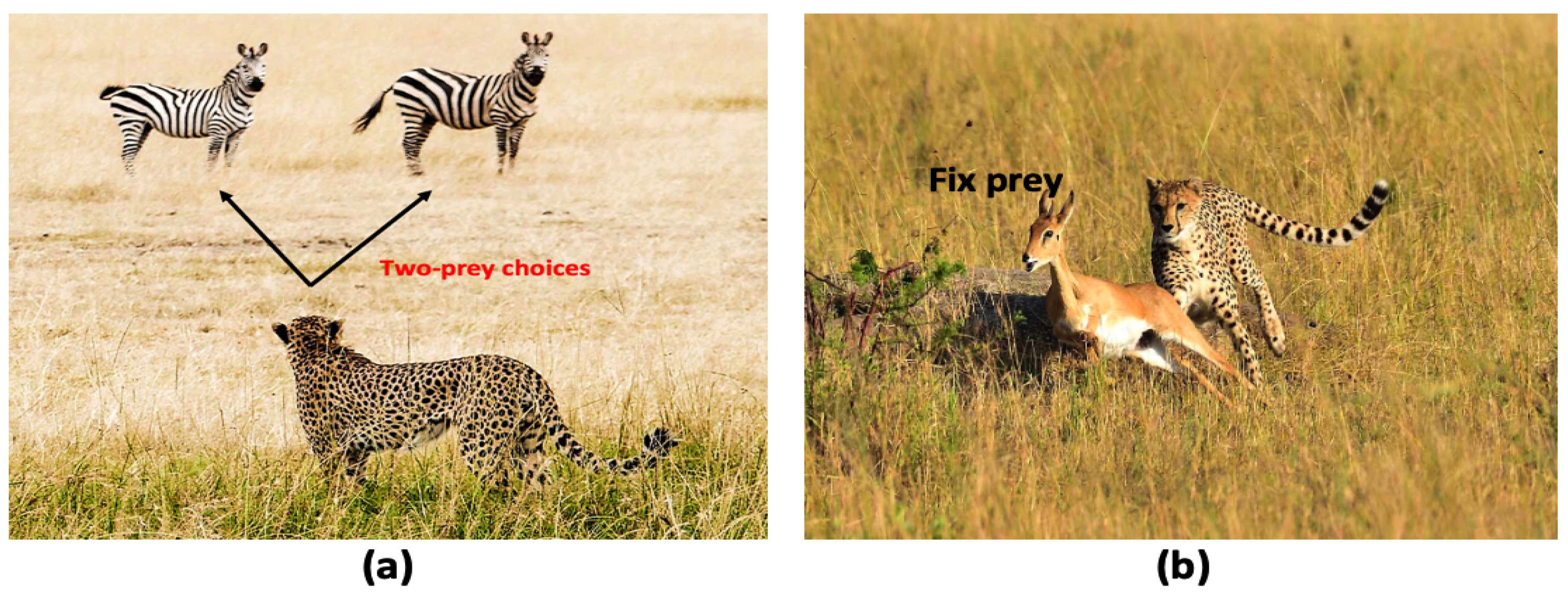
The presented functional Equation (1) with (2) has great importance in mathematical biology and learning theory. Such equations are used to investigate the response of animals in a two-choice situation, and the solution exists when a predator is fixed to one type of prey (see Figure 1).
On the other hand, the fixed point approach is regarded as a fundamental component and is a very effective method in nonlinear analysis due to its many critical implementations in various fields, including physics, engineering, computer science, biology, economics, and chemistry. This approach is widely used in mathematics to examine game-theoretic models, dynamical systems, statistical models, and differential equations. More specifically, this approach is mainly used to analyze certain integro-differential equations, functional equations, differential and integral equations, and fractional equations, which simplifies the process of obtaining computational solutions to such problems (for the details, see [40,41,42,43,44] and references therein).
In this work, our aim was to use the appropriate fixed point technique to demonstrate the existence of a unique solution to Equation (1) with (2). After that, we considered the stability of solutions to the suggested stochastic Equation (1) under the Hyers–Ulam (HU) and Hyers–Ulam–Rassias type (HUR) stability results. We provide three examples to emphasize the significance of our main conclusions.
Progress of this work requires the accomplishment of the following stated result, which guarantees the existence and uniqueness of fixed points of certain self-maps of metric spaces and provides a constructive method to find those fixed points.
Theorem 1
(Banach fixed point theorem). Let be a complete metric space and be a Banach contraction mapping (shortly, BCM) defined by
for some and for all Then has one fixed point. Furthermore, the Picard iteration in which is defined by for all , where , converges to the unique fixed point of .
2. Main Results
Let with where We denote a class having the continuous real-valued functions with and , where
for all .
We shall use the following conditions to prove the main results:
- ()
- ()
- The mappings are Banach contraction mappings with contractive coefficients , respectively, and satisfy the following conditions
- ()
- For a function , we have that for every with , there is a unique with and for some .
- ()
- For , we have that for every with , there is a unique with and for some .
Now, we begin with the outcome stated below.
Theorem 2.
Consider the stochastic functional Equation (1) associated with (2). Suppose that the conditions () and () are satisfied and there exists an where
Then, for each and for all a self-mapping from to is a BCM which is defined by
Proof.
Let . For each such that , and we obtain
From the above equation, we can write
As are Banach contraction mappings, i.e.,
where are contractive coefficients, respectively. Thus, by using the above relation with the definition of norm (4), we have
where is given in (6). This gives that
It follows from that is a BCM. This completes the proof. □
Theorem 3.
Consider the Equation (1) with (2). Suppose that the conditions () and () are satisfied and there exists an where Υ is given in (6). The mapping is a BCM, which is defined in (7). Thus, the proposed problem (1) associated with (2) has a unique solution in . Moreover, the iteration in () given by
converges to the unique solution of (1).
Proof.
As is a BCM, we obtain the outcome of this result by combining Theorem 2 with the Banach fixed point theorem. □
Here, we shall look at different conditions. If are Banach contraction mappings with contractive coefficients , respectively, then by Theorems 2 and 3, the outcomes are as follows.
Corollary 1.
Corollary 2.
Consider the Equations (1) and (2). Assume that the condition () is satisfied and there exists an . The mapping is a BCM, which is defined in (9). Thus, the proposed problem (1) associated with (2) has a unique solution in . Additionally, the iteration in () is defined as
converges to the unique solution of (1).
3. Stability Analysis
Here, we shall discuss the stability of the solution to the Equation (1) (see [47,48,49,50,51] for the details).
Theorem 4.
In light of Theorem 2’s assumptions, the equation where is defined as
for all and has HUR stability (defined in ()).
Proof.
Let such that . By using Theorem 2, we have a unique , such that . Thus, we obtain
where is defined in (6), and so by , we have
□
We gain the following conclusion about the HU stability from the aforementioned investigation.
Corollary 3.
In light of Theorem 2’s assumptions, the equation where is given by
for all and has HU stability (defined in ()).
4. Some Illustrative Examples
Here, we provide the following examples to justify our findings.
Example 1.
Consider the stochastic functional equation given below
for all with and . If we set the mappings by
for all , so (1) decreases to the Equation (13). It is easy to see that the mappings satisfy (), i.e.,
for all , where are contractive coefficients, respectively. Here, if () is satisfied with
then the mapping defined on (13) is a BCM. Thus, all conditions of Theorem 2 are fulfilled and, therefore, we obtain the existence of a solution to the functional Equation (13).
For a unique solution of (13), we define as a starting approximation (whereas is an identity function), then by Theorem 3, we obtain the convergence of the following iteration process:
for all .
On the other hand, as , we obtain
If a function satisfies the inequality
then Theorem 4 implies that there exists a unique , such that
Example 2.
Consider the functional equation given below
for all with and . If we set the mappings by
for all , so (1) decreases to the Equation (14). It is easy to see that the mappings satisfy (), i.e.,
for all , where are contractive coefficients, respectively. Here, if () is satisfied with
then the mapping defined on (14) is a BCM. Thus, it fulfills all the conditions of Corollary 1 and, therefore, we obtain the results related to the existence of a solution to the functional Equation (14).
If we define as a starting approximation (whereas is an identity function), then by Corollary 2, we have a unique solution of (14) followed by the iteration process stated below:
for all .
As , we have
If a function satisfies the inequality
then Theorem 4 implies that there exists a unique , such that
Example 3.
Consider the functional equation given below
for all and . If we set the mappings by
for all , so (1) decreases to the Equation (15). It is easy to see that the mappings satisfy (), i.e.,
for all , where are contractive coefficients, respectively. Here, if () is satisfied with
then the mapping defined on (15) is a BCM. Thus it fulfills all the conditions of Theorem 2 and, therefore, we obtain the results related to the existence of a solution to the functional Equation (15).
If we define as a starting approximation (whereas is an identity function), then by Theorem 2, we have a unique solution of (15) followed by the iteration process stated below:
for all .
As , we have
If a function satisfies the inequality
then Theorem 4 implies that there exists a unique , such that
5. Conclusions
In population biology, predator–prey or host–parasite relationships are arguably the most often simulated phenomena. According to such models, a predator has two prey options, and the solution is determined when the predator is drawn to a certain prey type. In this research, we presented a generic functional equation that can cover numerous learning theory models in the current study. Additionally, we analyzed the solution to the proposed stochastic equation for its existence, uniqueness, and stability. To demonstrate the significance of our findings, we presented two examples. Our method is novel and can be applied to many mathematical models associated with mathematical psychology and learning theory.
Finally, we present the following open problems for those who are interested in this research.
Question 1: what would happen if a predator does not approach any prey and remains stuck to its original position?
Question 2: is there another way to establish the conclusions from Theorems 2 and 3?
Author Contributions
Conceptualization, A.T., W.A. and Z.D.M.; methodology, A.T., W.A., A.S. and R.G.; validation, A.T., R.G., Z.D.M. and W.A.; formal analysis, A.T. and R.G.; writing—original draft preparation, A.T., W.A., A.S. and Z.D.M.; funding acquisition, A.S. All authors have read and agreed to the published version of the manuscript.
Funding
This research received no external funding.
Institutional Review Board Statement
Not applicable.
Informed Consent Statement
Not applicable.
Data Availability Statement
Not applicable.
Conflicts of Interest
The authors declare no conflict of interest.
References
- Bazykin, A.D. Nonlinear Dynamics of Interacting Populations; World Scientific: Singapore, 1998. [Google Scholar]
- Ma, Z.; Wang, W. Asymptotic behavior of predator–Prey system with time dependent coefficients. Appl. Anal. 1989, 34, 79–90. [Google Scholar]
- Chen, F.; Shi, C. Global attractivity in an almost periodic multi-species nonlinear ecological model. Appl. Math. Comput. 2006, 180, 376–392. [Google Scholar] [CrossRef]
- Yuan, S.; Wu, D.; Lan, G.; Wang, H. Noise-induced transitions in a nonsmooth Producer–Grazer model with stoichiometric constraints. Bull. Math. Biol. 2020, 82, 1–22. [Google Scholar] [CrossRef] [PubMed]
- Yu, X.; Yuan, S.; Zhang, T. Survival and ergodicity of a stochastic phytoplankton–zooplankton model with toxin-producing phytoplankton in an impulsive polluted environment. Appl. Math. Comput. 2019, 347, 249–264. [Google Scholar] [CrossRef]
- Zhang, T.; Liu, X.; Meng, X.; Zhang, T. Spatio-temporal dynamics near the steady state of a planktonic system. Comput. Math. Appl. 2018, 12, 4490–4504. [Google Scholar] [CrossRef]
- Xu, C.; Yuan, S.; Zhang, T. Global dynamics of a predator–prey model with defense mechanism for prey. Appl. Math. Lett. 2016, 62, 42–48. [Google Scholar] [CrossRef]
- Tian, Y.; Zhang, T.; Sun, K. Dynamics analysis of a pest management prey–predator model by means of interval state monitoring and control. Nonlinear Anal. Hybrid Syst. 2017, 23, 122–141. [Google Scholar] [CrossRef]
- Liu, M.; He, X.; Yu, J. Dynamics of a stochastic regime-switching predator–prey model with harvesting and distributed delays. Nonlinear Anal. Hybrid Syst. 2018, 28, 87–104. [Google Scholar] [CrossRef]
- Yu, X.; Yuan, S.; Zhang, T. The effects of toxin-producing phytoplankton and environmental fluctuations on the planktonic blooms. Nonlinear Dyn. 2018, 91, 1653–1668. [Google Scholar] [CrossRef]
- Zhao, S.; Yuan, S.; Wang, H. Threshold behavior in a stochastic algal growth model with stoichiometric constraints and seasonal variation. J. Differ. Equ. 2020, 9, 5113–5139. [Google Scholar] [CrossRef]
- Zhu, G.; Meng, X.; Chen, L. The dynamics of a mutual interference age structured predator–prey model with time delay and impulsive perturbations on predators. Appl. Math. Comput. 2010, 216, 308–316. [Google Scholar] [CrossRef]
- Diz-Pita, É.; Otero-Espinar, M.V. Predator–Prey Models: A Review of Some Recent Advances. Mathematics 2021, 9, 1783. [Google Scholar] [CrossRef]
- Banerjee, M.; Mukherjee, N.; Volpert, V. Prey-predator model with a nonlocal bistable dynamics of prey. Mathematics 2018, 6, 41. [Google Scholar] [CrossRef] [Green Version]
- Yang, R.; Zhao, X.; An, Y. Dynamical analysis of a delayed diffusive predator–prey model with additional food provided and anti-predator behavior. Mathematics 2022, 10, 469. [Google Scholar] [CrossRef]
- Bai, D.; Zhang, X. Dynamics of a predator–prey model with the additive predation in prey. Mathematics 2022, 10, 655. [Google Scholar] [CrossRef]
- Iqbal, N.; Wu, R. Pattern formation by fractional cross-diffusion in a predator-prey model with Beddington-DeAngelis type functional response. Int. J. Mod. Phys. A 2019, 33, 1950286. [Google Scholar] [CrossRef]
- Jia, W.; Xu, Y.; Li, D.; Hu, R. Stochastic analysis of predator-prey models under combined Gaussian and poisson white noise via stochastic averaging method. Entropy 2021, 23, 1208. [Google Scholar] [CrossRef]
- Rosenzweig, M.L.; Macarthur, R.H. Graphical representation and stability conditions of predator-prey Interactions. Am. Nat. 1963, 97, 209–223. [Google Scholar] [CrossRef]
- Zhu, W.Q.; Yang, Y.Q. Stochastic averaging of quasi-nonintegrable-Hamiltonian systems. J. Appl. Mech.-Trans. ASME 1997, 64, 157–164. [Google Scholar] [CrossRef]
- Roberts, J.B.; Spanos, P.D. Stochastic averaging: An approximate method of solving random vibration problems. Int. J. Non-Linear Mech. 1986, 21, 111–134. [Google Scholar] [CrossRef]
- Zhu, W. Stochastic averaging methods in random vibration. Appl. Mech. Rev. 1988, 41, 189–199. [Google Scholar] [CrossRef]
- Huang, Z.L.; Zhu, W.Q. Stochastic averaging of quasi-integrable Hamiltonian systems under combined harmonic and white noise excitations. Int. J. Non-Linear Mech. 2004, 39, 1421–1434. [Google Scholar] [CrossRef]
- Jia, W.T.; Xu, Y.; Liu, Z.H.; Zhu, W.Q. An asymptotic method for quasi-integrable Hamiltonian system with multi-time-delayed feedback controls under combined Gaussian and Poisson white noises. Nonlinear Dyn. 2017, 90, 2711–2727. [Google Scholar] [CrossRef]
- Pan, S.S.; Zhu, W.Q. Dynamics of a prey-predator system under Poisson white noise excitation. Acta Mech. Sin. 2014, 30, 739–745. [Google Scholar] [CrossRef]
- Jia, W.T.; Xu, Y.; Li, D.X. Stochastic dynamics of a time-delayed ecosystem driven by Poisson white noise excitation. Entropy 2018, 20, 143. [Google Scholar] [CrossRef] [PubMed] [Green Version]
- Gu, X.D.; Zhu, W.Q. Stochastic optimal control of predator-prey ecosystem by using stochastic maximum principle. Nonlinear Dyn. 2016, 85, 1177–1184. [Google Scholar] [CrossRef]
- Bush, A.A.; Wilson, T.R. Two-choice behavior of paradise fish. J. Exp. Psych. 1956, 51, 315–322. [Google Scholar] [CrossRef]
- Bush, R.; Mosteller, F. Stochastic Models for Learning; Wiley: New York, NY, USA, 1955. [Google Scholar]
- Istrăţescu, V.I. On a functional equation. J. Math. Anal. Appl. 1976, 56, 133–136. [Google Scholar] [CrossRef]
- Berinde, V.; Khan, A.R. On a functional equation arising in mathematical biology and theory of learning. Creat. Math. Inform. 2015, 24, 9–16. [Google Scholar] [CrossRef]
- Turab, A.; Sintunavarat, W. On the solutions of the two preys and one predator type model approached by the fixed point theory. Sādhanā 2020, 45, 211. [Google Scholar] [CrossRef]
- Turab, A.; Sintunavarat, W. On the solution of the traumatic avoidance learning model approached by the Banach fixed point theorem. J. Fixed Point Theory Appl. 2020, 22, 50. [Google Scholar] [CrossRef]
- Turab, A.; Sintunavarat, W. On analytic model for two-choice behavior of the paradise fish based on the fixed point method. J. Fixed Point Theory Appl. 2019, 21, 56, Erratum in J. Fixed Point Theory Appl. 2020, 22, 82. [Google Scholar] [CrossRef]
- Turab, A.; Ali, A.; Park, C. A unified fixed point approach to study the existence and uniqueness of solutions to the generalized stochastic functional equation emerging in the psychological theory of learning. AIMS Math. 2022, 7, 5291–5304. [Google Scholar] [CrossRef]
- Turab, A.; Park, W.-G.; Ali, W. Existence, uniqueness, and stability analysis of the probabilistic functional equation emerging in mathematical biology and the theory of learning. Symmetry 2021, 13, 1313. [Google Scholar] [CrossRef]
- Debnath, P. A mathematical model using fixed point theorem for two-choice behavior of rhesus monkeys in a noncontingent environment. In Metric Fixed Point Theory; Debnath, P., Konwar, N., Radenović, S., Eds.; Forum for Interdisciplinary Mathematics; Springer: Singapore, 2021. [Google Scholar] [CrossRef]
- FUTURITY. 2019. Available online: https://www.futurity.org/predator-prey-cycles-coexistence-2238732/ (accessed on 25 March 2022).
- Geek Reply. 2015. Available online: https://geekreply.com/science/2015/09/09/predator-prey-ratio-may-reveal-a-new-law-of-nature (accessed on 25 March 2022).
- Aydi, H.; Karapinar, E.; Rakocevic, V. Nonunique fixed point theorems on b-metric spaces via simulation functions. Jordan J. Math. Stat. 2019, 12, 265–288. [Google Scholar]
- Karapinar, E. Ciric type nonunique fixed points results: A review. Appl. Comput. Math. Int. J. 2019, 1, 3–21. [Google Scholar]
- Alsulami, H.H.; Karapinar, E.; Rakocevic, V. Ciric type nonunique fixed point theorems on b-metric spaces. Filomat 2017, 31, 3147–3156. [Google Scholar] [CrossRef]
- Gopal, D.; Abbas, M.; Patel, D.K.; Vetro, C. Fixed points of α-type F-contractive mappings with an application to nonlinear fractional differential equation. Acta Math. Sci. 2016, 36, 957–970. [Google Scholar] [CrossRef]
- Lakzian, H.; Gopal, D.; Sintunavarat, W. New fixed point results for mappings of contractive type with an application to nonlinear fractional differential equations. J. Fixed Point Theory Appl. 2016, 18, 251–266. [Google Scholar] [CrossRef]
- Banach, S. Sur les operations dans les ensembles abstraits et leur applications aux equations integrales. Fund. Math. 1922, 3, 133–181. [Google Scholar] [CrossRef]
- Agarwal, P.; Jleli, M.; Samet, B. Banach contraction principle and applications. In Fixed Point Theory in Metric Spaces; Springer: Singapore, 2018; pp. 1–23. [Google Scholar] [CrossRef]
- Hyers, D.H.; Isac, G.; Rassias, T.M. Stability of Functional Equations in Several Variables; Birkhauser: Basel, Switzerland, 1998. [Google Scholar]
- Morales, J.S.; Rojas, E.M. Hyers-Ulam and Hyers-Ulam-Rassias stability of nonlinear integral equations with delay. Int. J. Nonlinear Anal. Appl. 2011, 2, 1–6. [Google Scholar]
- Rassias, T.M. On the stability of the linear mapping in Banach spaces. Proc. Am. Math. Soc. 1978, 72, 297–300. [Google Scholar] [CrossRef]
- Bae, J.H.; Park, W.G. A fixed point approach to the stability of a Cauchy-Jensen functional equation. Abstr. Appl. Anal. 2012, 2012, 205160. [Google Scholar] [CrossRef]
- Gachpazan, M.; Bagdani, O. Hyers-Ulam stability of nonlinear integral equation. Fixed Point Theory Appl. 2010, 927640, 1–6. [Google Scholar] [CrossRef] [Green Version]
Figure 1.
(a): A predator with two choices of prey [38]; (b): a predator fixed to one type of prey [39].

| Operators for reinforcement-extinction model | ||
| Animal’s Response | Outcome (Left side) | Outcome (Right side) |
| Reinforcement | ||
| Non-reinforcement | ||
| Operators for habit formation model | ||
| Animal’s Response | Outcome (Left side) | Outcome (Right side) |
| Reinforcement | ||
| Non-reinforcement | ||
Table 2.
Physical meaning of the parameters/operators.
| Parameter/Operator | Physical Meaning |
|---|---|
| State space | |
| Learning-rate parameters | |
| Probability of a chosen side | |
| Transition operators | |
| Final probability |
Publisher’s Note: MDPI stays neutral with regard to jurisdictional claims in published maps and institutional affiliations. |
© 2022 by the authors. Licensee MDPI, Basel, Switzerland. This article is an open access article distributed under the terms and conditions of the Creative Commons Attribution (CC BY) license (https://creativecommons.org/licenses/by/4.0/).
Share and Cite
MDPI and ACS Style
George, R.; Mitrović, Z.D.; Turab, A.; Savić, A.; Ali, W. On a Unique Solution of a Class of Stochastic Predator–Prey Models with Two-Choice Behavior of Predator Animals. Symmetry 2022, 14, 846. https://doi.org/10.3390/sym14050846
AMA Style
George R, Mitrović ZD, Turab A, Savić A, Ali W. On a Unique Solution of a Class of Stochastic Predator–Prey Models with Two-Choice Behavior of Predator Animals. Symmetry. 2022; 14(5):846. https://doi.org/10.3390/sym14050846
Chicago/Turabian StyleGeorge, Reny, Zoran D. Mitrović, Ali Turab, Ana Savić, and Wajahat Ali. 2022. "On a Unique Solution of a Class of Stochastic Predator–Prey Models with Two-Choice Behavior of Predator Animals" Symmetry 14, no. 5: 846. https://doi.org/10.3390/sym14050846
Note that from the first issue of 2016, this journal uses article numbers instead of page numbers. See further details here.