
Traveling Wave Solutions to the Nonlinear Evolution Equation Using Expansion Method and Addendum to Kudryashov’s Method


Department of Mathematics and Statistics, College of Science, Taif University, P.O. Box 11099, Taif 21944, Saudi Arabia
Symmetry 2021, 13(11), 2126; https://doi.org/10.3390/sym13112126
Submission received: 18 October 2021
/
Revised: 30 October 2021
/
Accepted: 3 November 2021
/
Published: 8 November 2021
(This article belongs to the Special Issue Ordinary and Partial Differential Equations: Theory and Applications II)
Abstract
:The inspection of wave motion and propagation of diffusion, convection, dispersion, and dissipation is a key research area in mathematics, physics, engineering, and real-time application fields. This article addresses the generalized dimensional Hirota–Maccari equation by using two different methods: the expansion method and Addendum to Kudryashov’s method to obtain the optical traveling wave solutions. By utilizing suitable transformations, the nonlinear pdes are transformed into odes. The traveling wave solutions are expressed in terms of rational functions. For certain parameter values, the obtained optical solutions are described graphically with the aid of Maple 15 software.
1. Introduction
The study of the traveling wave solutions plays a significant role in understanding and describing the characters of nonlinear problems in physical science. The elements of physical systems usually operate on multiple time scales [1]. Although closed form descriptions for nonlinear partial differential equations (nlpdes) of physical significance exist, we cannot obtain these forms explicitly. Such problems occur especially in various realistic problems in physical systems. In this scenario, we aim to investigate exact physically significant solutions, which are so important and useful due to their very wide application of nlpdes in fluid mechanics, fluid dynamics, quantum mechanics, bio-science, physics, chemistry, and other areas of engineering.
Modeling of wave motion has attracted many researchers due to its crucial role in ocean, coastal, naval and marine engineering. In addition, waves are considered to be the major source of environmental actions on beaches or floating structures for most geographical areas. Most problems of practical interest create physical phenomena in nature that are often nonlinear and can be described by fractional differential equations. For example, heat conduction systems, nonlinear chaotic systems, plasma waves, and diffusion processes are modeled by fractional mathematics and equations [2,3,4]. Therefore, numerous investigations have been conducted to develop new methods to solve such equations. For example, Choucha et al. [5] investigated problems of a nonlinear viscoelastic wave equation in the presence of distributed delay, strong damping and source terms. By considering suitable conditions, they obtained a blow-up result of solutions. The improved sub-equation method has been used by Zhong et al. [6] to obtain exact solutions for a wide range of nonlinear problems of fractional equations. By converting nonlinear problems of fractional and integer order equations with the modified Riemann–Liouville derivative into Riccati equations, they obtained exact solutions, including wave solutions, soliton solutions, and complex solutions. Simbanefayi et al. [7] obtained traveling wave solutions for the Korteweg–de Vries–Benjamin–Bona–Mahony equation using Lie symmetry and Jacobi elliptic function expansion methods. The main objective of the Lie symmetry method is to transform the governing equations to a simpler equation while maintaining the invariance of the original equation. Others have previously used different methods to find the traveling wave solutions for nonlinear evolution equations (nees) (see, for example, [8,9,10,11,12,13,14,15,16,17,18,19,20]).
Over the past few years, many researchers have explored several direct methods to solve nonlinear evolution equations. One of the popular examples of such methods is the Kudryashov method, which typically only performs the calculation without the need for the form of a specific function. Examples of Kudryashov methods include the extended Kudryashov method [21], the generalized Kudryashov method [22], and the new extended generalized Kudryashov method [23]. The generalized Kudryashov method by Kaplan et al. [22] does usefully apply to the nonlinear Jaulent–Miodek hierarchy and -dimensional Calogero–Bogoyavlenskii–Schiff equation. This method has successfully provided exact solutions to the nonlinear evolution equations. The Addendum to Kudryashov’s method is also among the Kudryashov methods and was introduced by [24]. This method is the general form of previous Kudryashov methods because the trial equation is proposed as the general form of the trial equations in other Kudryashov methods.
In this article, we construct the exact significant solutions for different types of cases of the -expansion method and akm. Both methods are used as powerful mathematical tools for constructing traveling wave solutions of nonlinear partial differential equations (see, for example, [20,21,22,23,24,25,26]).
For the purposes of discussion, we consider the nonlinear dimensional Hirota–Maccari equation [27]. Let x and y be the independent spatial variables and t be the time variable. Consider the complex and the real scalar fields and , respectively, satisfying the -dimensional Hirota–Maccari equation
In the last two decades, scientists have explored the Hirota–Maccari system using several approaches to efficiently compute and predict exact solutions. The approach by Painlevé has been applied successfully to construct the general solutions of certain nonlinear second-order equations [27]. Other methods that have been introduced include a new unified algebraic method [29], Weierstrass elliptic function expansion method [30] and extended trial method [31].
Here, we focus attention on using the expansion method and akm to predict and derive exact solutions of the Hirota–Maccari system. This paper is organized as follows. Section 2 presents the methodology of the -expansion method. Section 3 discusses the Hirota–Maccari equation. In addition, numerical computations are carried out by Maple to present the behavior of the optical traveling wave solution through figures. Section 4 addresses the -dimensional Hirota–Maccari equation by using Addendum to Kudryashov’s method (akm) to find the straddled solitary wave solution and the singular soliton solution and presents them in graphs.
2. Methodology of the Expansion Method
This section presents the procedure of the -expansion method. In the first step, we consider a nonlinear partial differential equation in the following form:
where represents an unknown function, and F is a polynomial function in and its partial derivatives. We define an appropriate traveling wave transformation as follows,
where c is the velocity of a traveling wave. By utilizing this appropriate traveling wave transformation (3), the nonlinear partial differential Equation (2) reduces to the ordinary differential equation (ode):
in which Q is a polynomial in and its total derivatives such that
We seek traveling wave solutions for a large class of Equation (4) in the following form:
where are arbitrary constants, N is a positive integer, and is the elementary function that satisfies the following ode:
where and are arbitrary constants. By taking the transformation , the nonlinear ode (6) can be written in the following form
The above Equation (7) is the generalized Riccati first ode’s. By taking this transformation , the generalized Riccati first ode’s (7) reduces to the following form
which can be solved by applying a separation of variables to obtain the following solutions:
- First, when and we have the hyperbolic function solutions:orwhere E is the integration constant.
- Second, when and we have solutions as:
- Third, when we obtain the periodic solutions as:or
- Fourth, when we obtain the solution as:
- Fifth, when we obtain the solution as:
Substituting Equation (5) into Equation (4) and using ode (6), the left-hand side is transferred to a polynomial in By equating the coefficient of this polynomial to zero, we obtain a system of algebraic equations that describes the model equations for and These algebraic system of equations are solved by means of the Maple software. Substituting the values of the parameters and the general solution of Equation (6) into Equation (5), we obtain the desired traveling wave solutions, as shown in Equation (2).
3. Application
The proposed method in the previous section is implemented successfully to the Hirota–Maccari system (1) to obtain explicit and exact traveling wave solutions. The traveling wave solutions of the Hirota–Maccari system (1) are expressed in the form [32]
where U and V are real functions, and c is the wave velocity, p is the frequency of the wave, while q and k are arbitrary constants. Using the traveling wave transformation (16) empowers us to transform the Hirota–Maccari system (1) into the following system of odes:
where By explicitly taking advantage of the homogeneous balance method [33], we balance the nonlinear term and the highest order derivative in Equation (17) to obtain the balance constant Therefore, the solution of Equation (17) takes the following form:
where are non-zero constants. Elementary algebra gives and as:
and
Substitute Equations (18)–(20) into Equation (17) and collect all terms with the same power of , for Then, setting the coefficients of , for to zero, yields:
Solving the above algebraic equations gives the values of the constants , and as:
Therefore, substituting these constants into the solution (18), we obtain
To obtain the optical traveling wave solutions for the Hirota–Maccari system, we substitute Equations (9)–(15) into Equation (23) to obtain the following five optical traveling wave solutions:
- Case 1: when and the complex and the real scalar fields can be expressed respectively as:and
- Case 2: when and the complex and the real scalar fields can be expressed, respectively, as:
- Case 3: when and the complex and the real scalar fields can be expressed respectively as:
- Case 4: when and the complex and the real scalar fields can be expressed, respectively, as:
- Case 5: when and the complex and the real scalar fields can be expressed, respectively, as:Figure 7 represents the singular Kink wave solution of the real part (Figure 7a) and imaginary part (Figure 7b) of (29a) and its projections (Figure 7c) and (Figure 7d), respectively, while the singular Kink wave solution (29b) and its projections are shown in Figure 8, for special values of parameters.
4. Addendum to Kudryashov’s Method (AKM) for -Dimensional Hirota–Maccari Equation
For nonlinear evolution equations (nlees), Kudryashov [34] introduced a new approach to find highly dispersive optical solitons. This method is intended to be used to perform the calculation without the need for the form of a specific function. Inspired by the work of Kudryashov [34], Zayed et al. [24] recently introduced the Addendum to Kudryashov’s method akm. One aim of this section is to apply this method to find the straddled solitary wave solutions and the singular soliton solutions of the -dimensional Hirota–Maccari equation.
For convenience, we start by presenting the main steps of the akm as follows:
- Step 1: Assuming that (17) has a solution in the following formwhere for are constants can be determined, and satisfies the node so thatwhere is an arbitrary constant. We can verify that Equation (31) can be written in the form:where A represents a non- zero real number, T is a natural number, and .
- Step 2: The relation between N and T can be calculated as follows: Setting then , , hence and
In the following, we present two cases to find the straddled solitary wave solutions and the singular soliton solutions of Equation (17):
- Case 1. Setting hence Then, we deduce from Equation (33) thatwhere and are constants and Substituting Equations (34) and (31) into Equation (17) and collecting all the transactions of this term for ( and ), and setting them to zero, leads to a system of equations that can be solved to obtain:andprovided Substituting Equations (35) and (32) into Equation (34), and calculating the straddled solitary solution of Equation (17) gives:andprovide In particular, setting in Equation (38), we obtain the singular soliton solution to Equation (17) asand
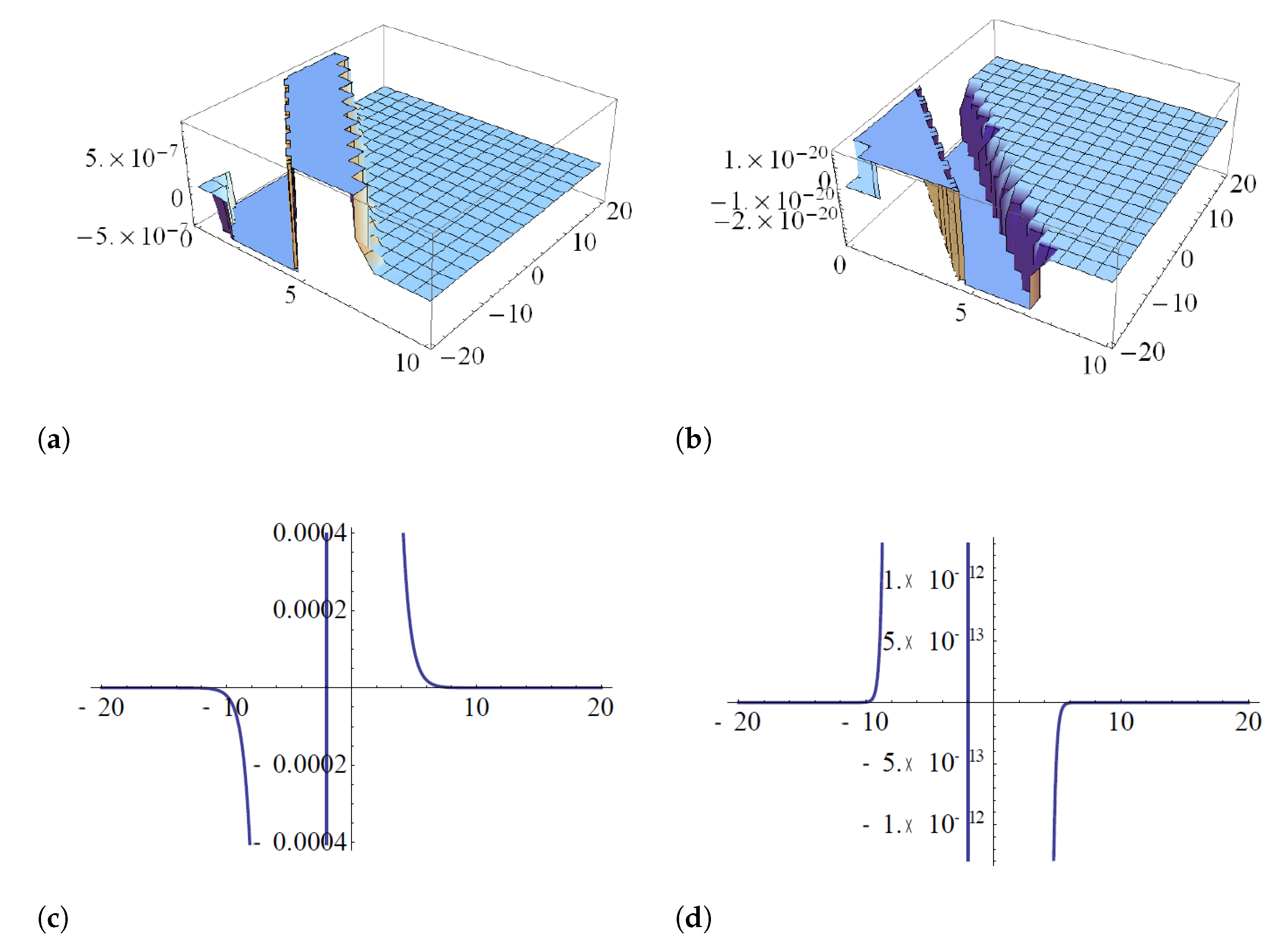
- Case 2. Setting hence Then, we deduce from Equation (30) that Equation (17) has solutions in following form:where , and are constants, and Substituting Equations (41) and (12) into Equation (17) and collecting all the transactions of this term for ( and ), and setting them to zero, we obtain a system of equations that can be solved to obtain the following results:andprovided Substituting Equations (42) and (43) into Equation (41), and calculating the straddled solitary solution of Equation (17) leads toandproviding In particular, setting in Equation (38), we obtain the singular soliton solution to Equation (17) asandNote that by choosing different values for the parameters T and N, we can obtain several solitary wave solutions of Equation (17).
Figure 9 shows the straddled solitary solution (37) when the velocity of the soliton is and the frequency is when Figure 9c,d shows the straddled solitary solution, which is a singular solution at . In addition, Figure 10 shows the straddled solitary solution (38), and Figure 10c,d shows the singular solutions at .
5. Conclusions
The search for exact solutions for nees has attracted the attention of many scientists in physics and mathematics. In this paper, I investigate the optical traveling wave solutions to a nonlinear evolution equation in mathematical physics, namely for the -dimensional Hirota–Maccari equation by means of the expansion method. Additionally, by following the method of the Addendum to Kudryashov’s method akm, introduced by Zayed et al. [24], Section 4 analogously derives the straddled solitary wave solution and the singular soliton solution of the -dimensional Hirota–Maccari Equation (1), which is presented with the support of graphs. The resulting solutions indicate that the proposed approach promises to empower us to address a wide class of nonlinear evolution equations arising in mathematical physics. The optical wave solutions obtained in this paper is just one important example of solutions that can have the potential to empower systematic analysis and understanding of the nonlinear evolution equation in many fields used widely in engineering and science.
Funding
This research received no external funding.
Data Availability Statement
Not applicable.
Acknowledgments
Taif University Researchers Supporting Project number (TURSP-2020/304), Taif University, Taif, Saudi Arabia.
Conflicts of Interest
The author declares no conflict of interest.
References
- Dolbow, J.; Khaleel, M.A.; Mitchell, J. Multiscale Mathematics Initiative: A Roadmap; Report from the 3rd DoE Workshop on Multiscale Mathematics, Technical Report; Department of Energy: Washington, DC, USA, 2004. Available online: http://www.sc.doe.gov/ascr/mics/amr (accessed on 8 November 2021).
- Baleanu, D.; Machado, A.T.; Luo, A.C.J. Fractional Dynamics Control; Springer Science & Business Media: New York, NY, USA, 2011; pp. 49–57. [Google Scholar]
- Boudjehem, B.; Boudjehem, D. Parameter tuning of a fractional-order PI Controller using the ITAE Criteria. Fractional Dyn. Control 2011, 49–57. [Google Scholar] [CrossRef]
- Alotaibi, H. Developing Multiscale Methodologies for Computational Fluid Mechanics. Ph.D. Thesis, The University of Adelaide, Adelaide, Australia, 2017. [Google Scholar]
- Choucha, A.; Ouchenane, D.; Boulaaras, S. A Backlund transformation and the inverse scattering transform method for the generalised Vakhnenko equation. Nonlinear Funct. Anal. 2020, 1–10. [Google Scholar] [CrossRef]
- Zhong, B.; Jiang, J.; Feng, Y. New exact solutions of fractional Boussinesq-like equations. Commun. Optim. Theory 2020, 1–17. [Google Scholar] [CrossRef]
- Simbanefayi, I.; Khalique, C.M. Travelling wave solutions and conservation laws for the Korteweg-de Vries-Bejamin-Bona-Mahony equation. Results Phys. 2018, 8, 57–63. [Google Scholar] [CrossRef]
- Vakhnenko, V.O.; Parkes, E.J.; Morrison, A.J. A Backlund transformation and the inverse scat-tering transform method for the generalised Vakhnenko equation. Chaos Solitons Fractals 2003, 17, 683–692. [Google Scholar] [CrossRef]
- Wazwaz, A.M. A sine-cosine method for handlingnonlinear wave equations. Math. Comput. Model. 2004, 40, 499–508. [Google Scholar] [CrossRef]
- Duffy, B.R.; Parkes, E.J. Traveling solitary wave solutions to a seventh-order generalized KdV equation. Phys. Lett. A 1996, 214, 271–272. [Google Scholar] [CrossRef]
- Fan, E.G. Extended tanh-function method and its applications to nonlinear equations. Phys. Lett. A 2000, 277, 212–218. [Google Scholar] [CrossRef]
- Zayed, E.M.; Gepreel, K.A. The modified (G/G) -expansion method and its applications to construct exact solutions for nonlinear PDEs. WSEAS Trans. Math. 2011, 10, 270–278. [Google Scholar]
- Ebadi, G.; Biswas, A. The G′/G method and topological Solitons solution of the K(m, n) equation. Commun. Nonlinear Sci. Numer. Simul. 2011, 16, 2377–2382. [Google Scholar] [CrossRef]
- He, J.H.; Wu, X.H. Exp-function method for nonlinear wave equations. Chaos Solitons Fractals 2006, 30, 700–708. [Google Scholar] [CrossRef]
- Cariello, F.; Tabor, M. Similarity reductions from extended Painleve’ expansions for nonin-tegrable evolution equations. Phys. D 1991, 53, 59–70. [Google Scholar] [CrossRef]
- Abdou, M.A. The extended F-expansion method and its application for a class of nonlinear evolution equations. Chaos Solitons Fractals 2007, 31, 95–104. [Google Scholar] [CrossRef]
- Jawad, A.J.; Petkovic, M.D.; Biswas, A. Modified simple equation method for nonlinear evo-lution equations. Appl. Math. Comp. 2010, 217, 869–877. [Google Scholar] [CrossRef]
- Zayed, E.M.; Arnous, A.H. Exact solutions of the nonlinear ZK-MEW and the Potential YTSF equations using the modified simple equation method. AIP Conf. Proc. ICNAAM 2012, 1479, 2044–2048. [Google Scholar]
- Taghizadeh, N.; Mirzazadeh, M. The Modified Extended Tanh Method with the Riccati Equa-tion for Solving Nonlinear Partial Differential Equations. Math. Aeterna 2012, 2, 145–153. [Google Scholar]
- Hafez, M.G.; Alam, M.N.; Akber, M.A. Application of the exp(−ϕ(ξ)))-expansion method to find exact solutions for the solitary wave equation in an unmagnetized dusty plasma. World Appl. Sci. J. 2014, 32, 2150–2155. [Google Scholar]
- Ege, S.M.; Misirli, E. Extended Kudryashov Method for Fractional Nonlinear Differential Equations. Math. Sci. Appl. 2018, 6, 19–28. [Google Scholar] [CrossRef]
- Kaplan, M.; Bekir, A.; Akbulut, A. A generalized Kudryashov method to some nonlinear evolution equations in mathematical physics. Nonlinear Dyn. 2016, 85, 2843–2850. [Google Scholar] [CrossRef]
- Zayed, E.M.; Shohib, R.M.; Alngar, M.E. New extended generalized Kudryashov method for solving three nonlinear partial differential equations. Nonlinear Anal. Model. Control 2020, 25, 598–617. [Google Scholar] [CrossRef]
- Zayed, E.M.E.; Alngar, M.E.M.; Biswas, A.; Kara, A.H.; Ekici, M.; Alzahrani, A.K.; Belic, M.R. Cubicquartic optical solitons and conservation laws with Kudryashov’s sextic power-law of refractive index. Optik 2021, 227, 166059. [Google Scholar] [CrossRef]
- Hafez, M.G.; Alam, M.N.; Akber, M.A.; Roshid, H.O. Exact traveling wave solutions of the (3 + 1)-Dimensional mkdv-zk and the (2 + 1)-Dimensional Burgers equations via exp(−ϕ(ξ)))-expansion method. Alex Eng. 2015, 54, 635–644. [Google Scholar]
- Hafez, M.G.; Ali, M.Y.; Chowdary, M.K.; Kauser, M.A. Application of the exp(−ϕ(ξ)))-expansion method for solving nonlinear TRLW and Gardner equations. Int. J. Math. Comput. 2016, 27, 44–56. [Google Scholar]
- Liang, Z.F.; Tang, X.Y. Modulational instability and variable separation solution for a general-ized (2+1)-dimensional Hirota equation. Chin. Phys. Lett. 2010, 27, 1–4. [Google Scholar]
- Hirota, R. Exact evelope-soliton solutions of a nonlinear wave equation. J. Math. Phys. 1973, 14, 805–809. [Google Scholar] [CrossRef]
- Fan, E. Uniformly constructing a series of explicit exact solutions to non-linear equations in mathematical physics. Chaos Solitons Fractals 2003, 16, 819–839. [Google Scholar] [CrossRef]
- Chen, Y.; Yan, Z. The Weierstrass elliptic function expansion method and its applications in nonlinear wave equations. Chaos Solitons Fractals 2006, 29, 948–964. [Google Scholar] [CrossRef] [Green Version]
- Jia, T.T.; Chai, Y.Z.; Hao, H.Q. Multi-soliton solutions and Breathers for the generalized coupled nonlinear Hirota equations via the Hirota method. Superlattices Microstruct. 2006, 127, 1848–1859. [Google Scholar] [CrossRef]
- Gepreel, K.A. Exact Soliton Solutions for Nonlinear Perturbed Schrödinger Equations with Nonlinear Optical Media. Appl. Sci. 2020, 10, 8929. [Google Scholar] [CrossRef]
- Wang, M.; Li, X.Z. Extended F-expansion method and periodic wave solutions for the gen-eralized Zakharov equations. Phys. Lett. A 2005, 343, 48–54. [Google Scholar] [CrossRef]
- Kudryashov, N.A. Method for finding highly dispersive optical solitons of nonlinear differential equations. Optik 2020, 206, 163550. [Google Scholar] [CrossRef]
Figure 1.
Periodic wave solution of the real part (a) and imaginary part (b) of (24a) and its projections (c,d), respectively, when and .
Figure 1.
Periodic wave solution of the real part (a) and imaginary part (b) of (24a) and its projections (c,d), respectively, when and .
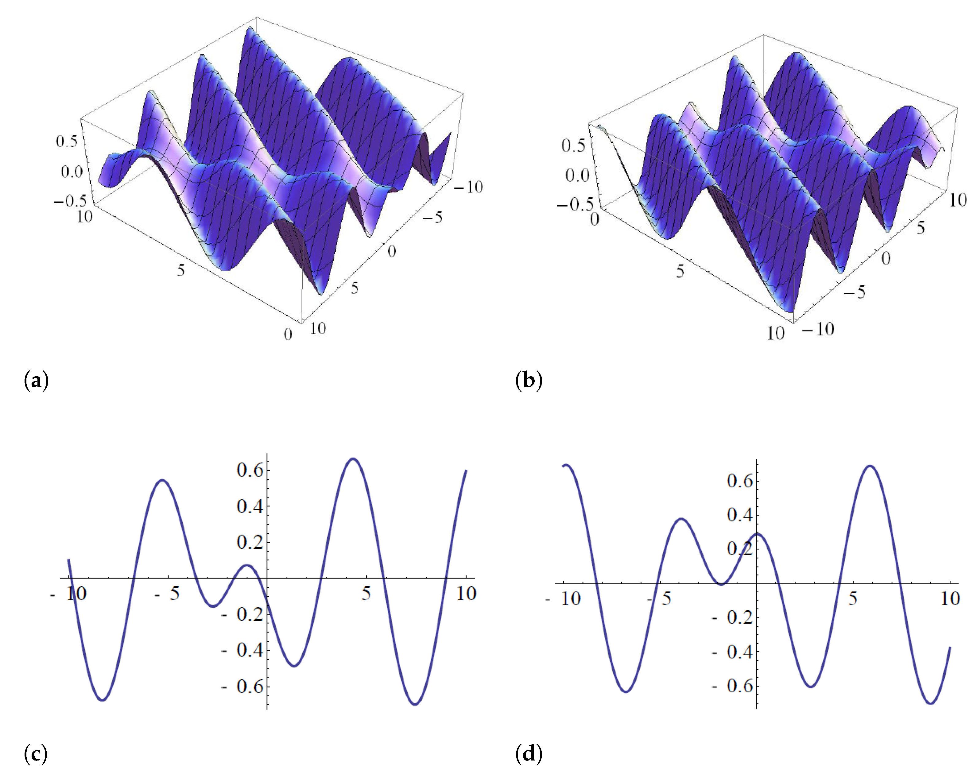
Figure 2.
Bright wave solution (24b) (left) and its projections (right), when and .
Figure 2.
Bright wave solution (24b) (left) and its projections (right), when and .
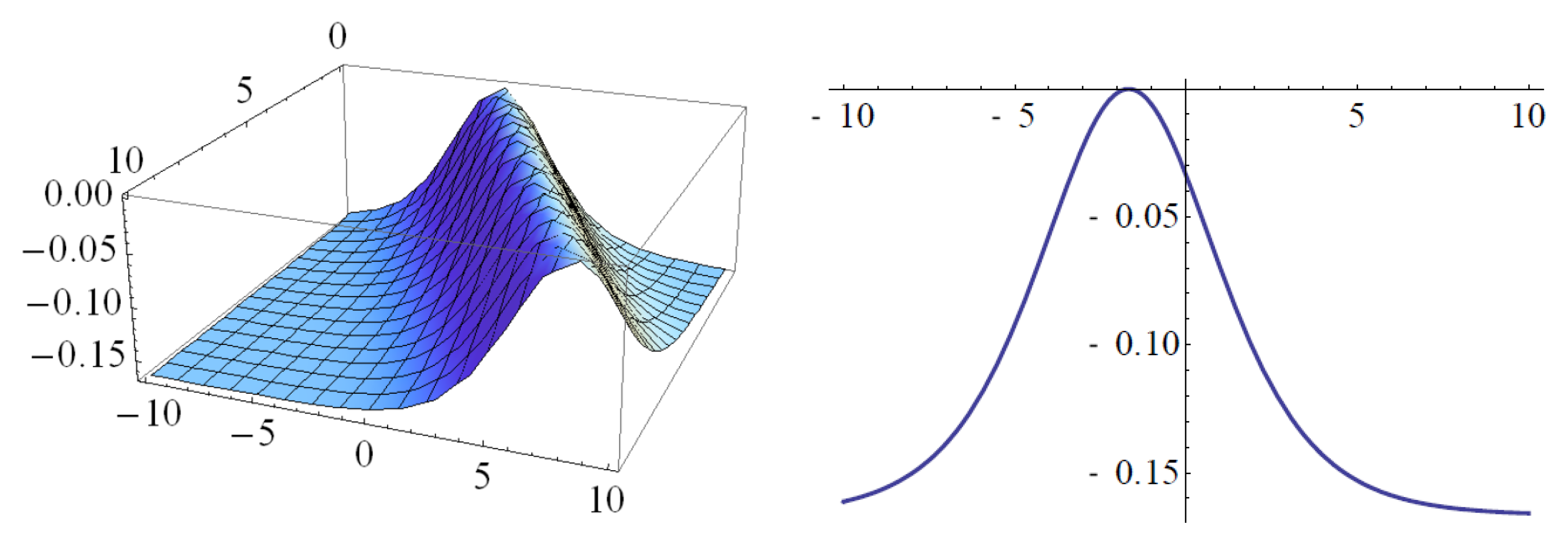
Figure 3.
The singular solitary wave solution of the real part (a) and imaginary part (b) to (26a) and its projections (c,d), respectively, when and .
Figure 3.
The singular solitary wave solution of the real part (a) and imaginary part (b) to (26a) and its projections (c,d), respectively, when and .
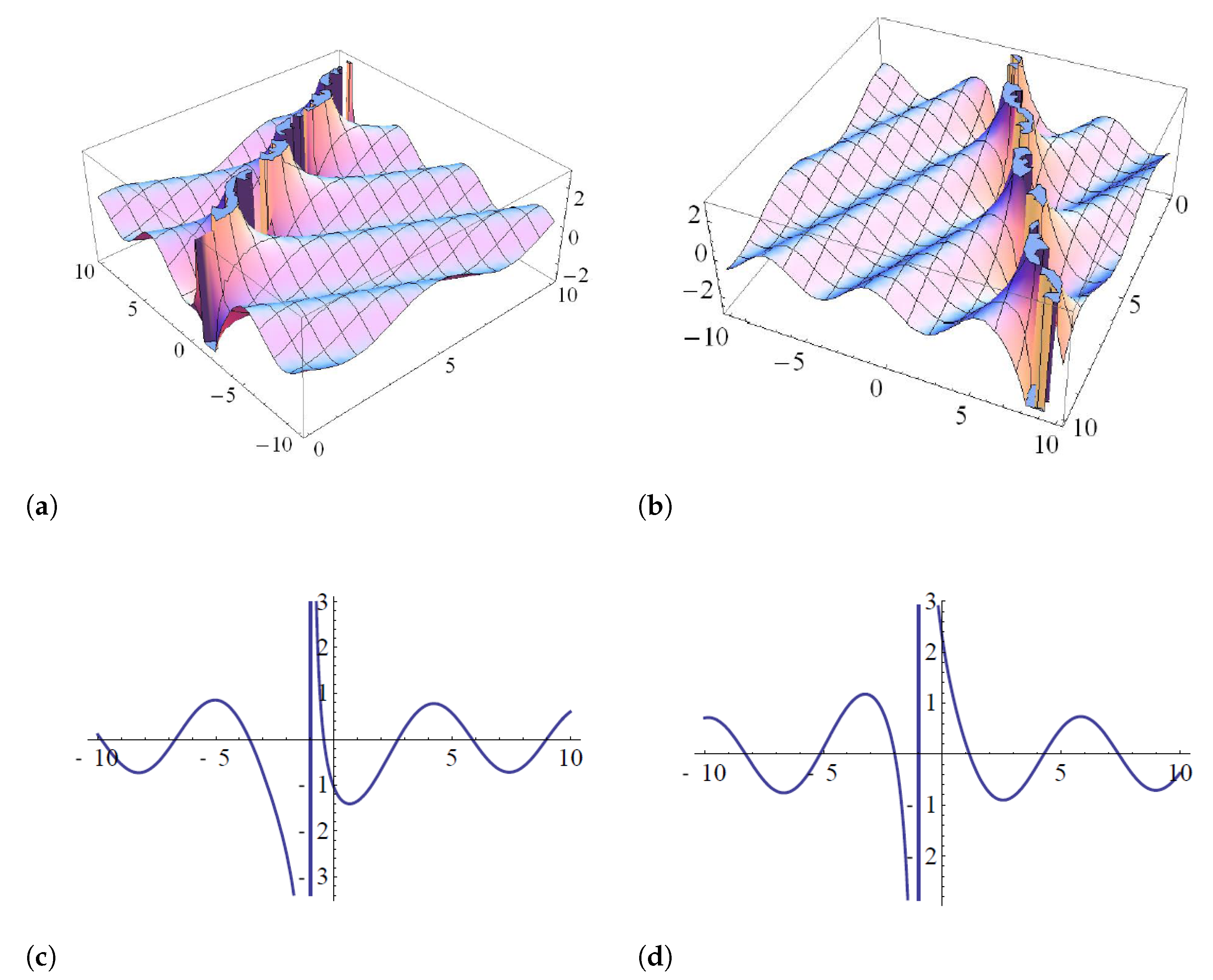
Figure 4.
The singular Kink wave solution (26b) (left) and its projections (right), when and .
Figure 4.
The singular Kink wave solution (26b) (left) and its projections (right), when and .
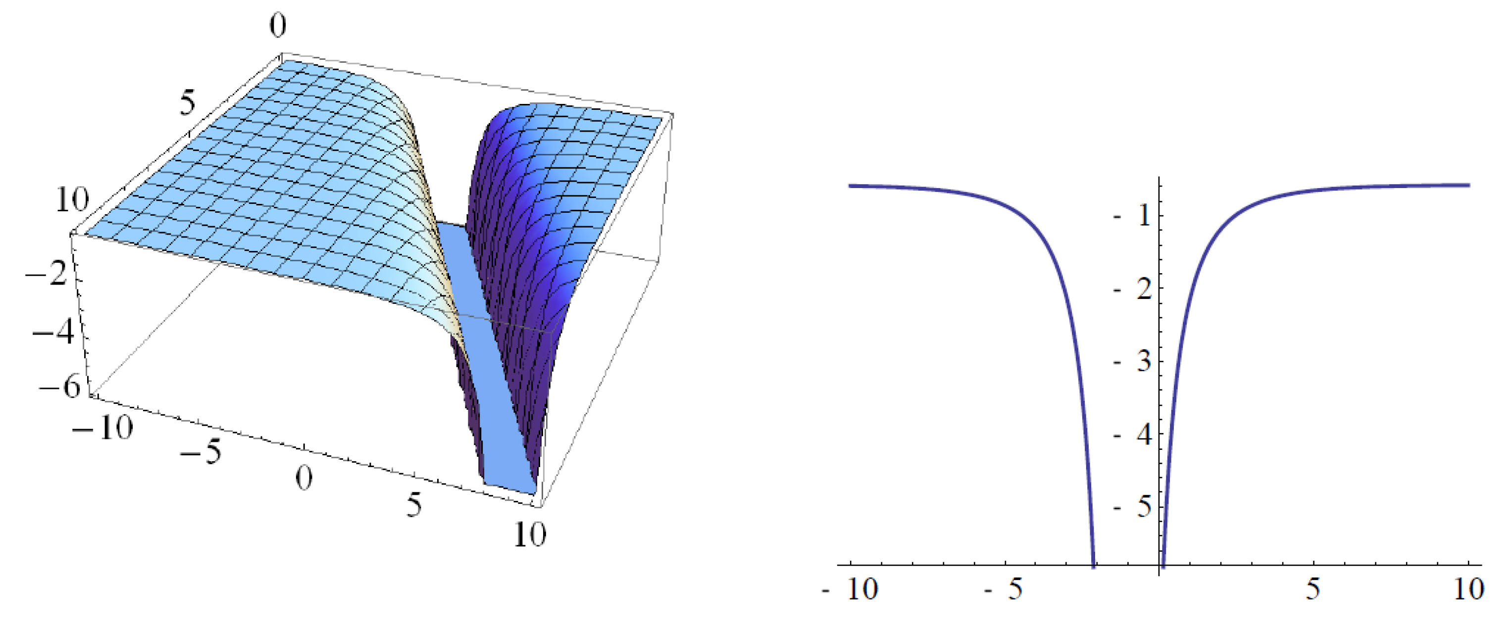
Figure 5.
The periodic wave solution of the real part (a) and imaginary part (b) to (27b) and its projections (c,d), respectively, when and .
Figure 5.
The periodic wave solution of the real part (a) and imaginary part (b) to (27b) and its projections (c,d), respectively, when and .

Figure 6.
The singular Kink solution of (27a) (left) and its projections (right), when and .
Figure 6.
The singular Kink solution of (27a) (left) and its projections (right), when and .
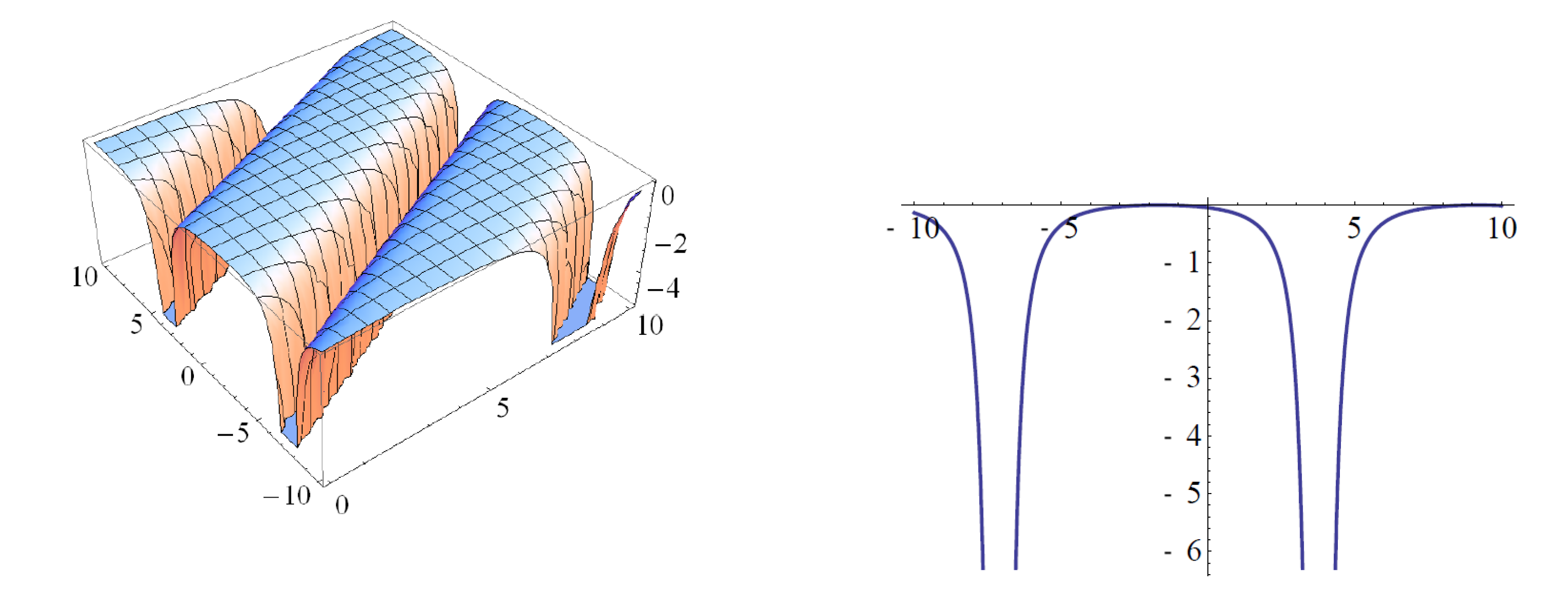
Figure 7.
The singular Kink solution of the real part (a) and imaginary part (b) to (29a) and its projections (c,d), respectively, when and .
Figure 7.
The singular Kink solution of the real part (a) and imaginary part (b) to (29a) and its projections (c,d), respectively, when and .
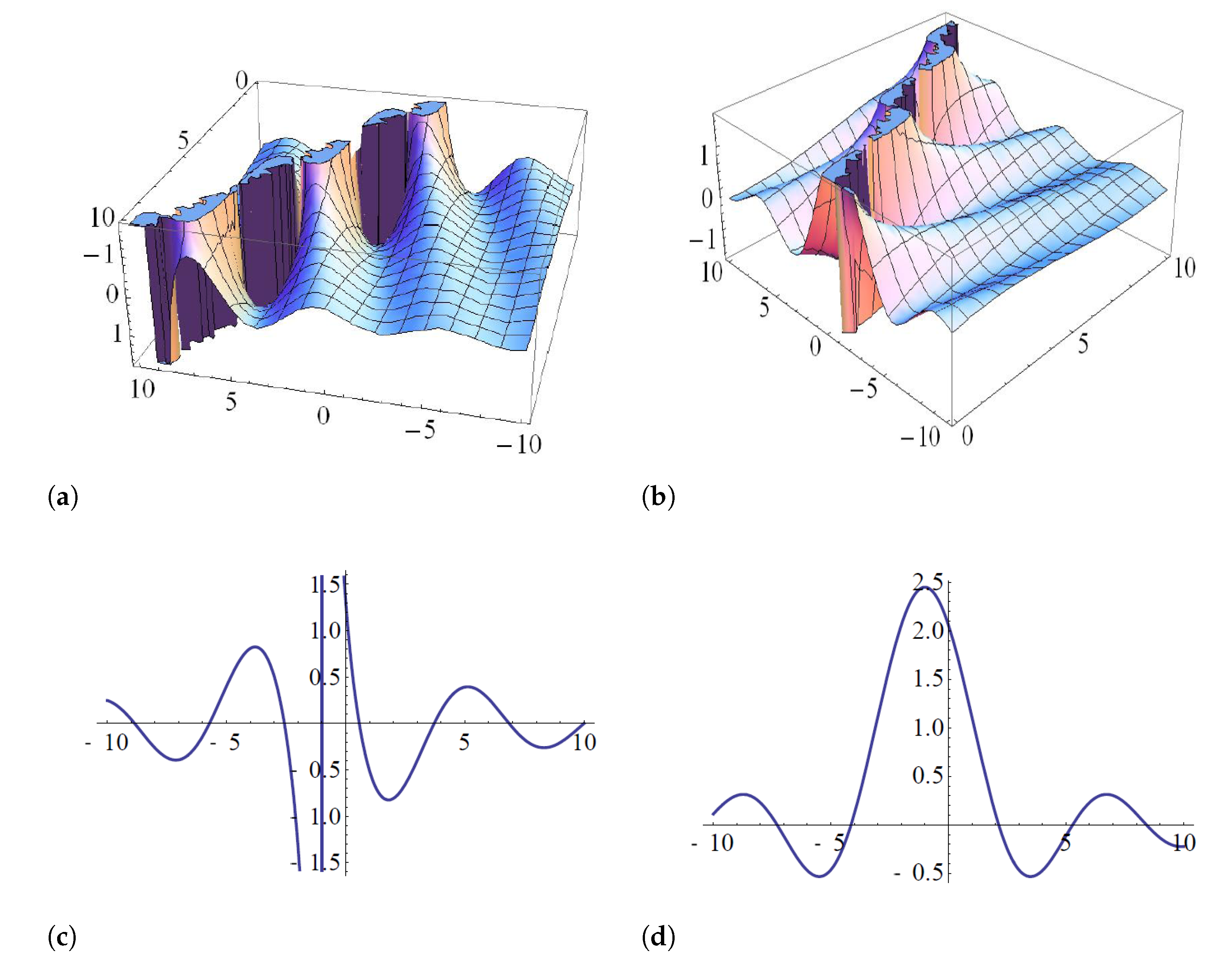
Figure 8.
The singular Kink solution of (29b) (left) and its projections (right), when and .
Figure 8.
The singular Kink solution of (29b) (left) and its projections (right), when and .
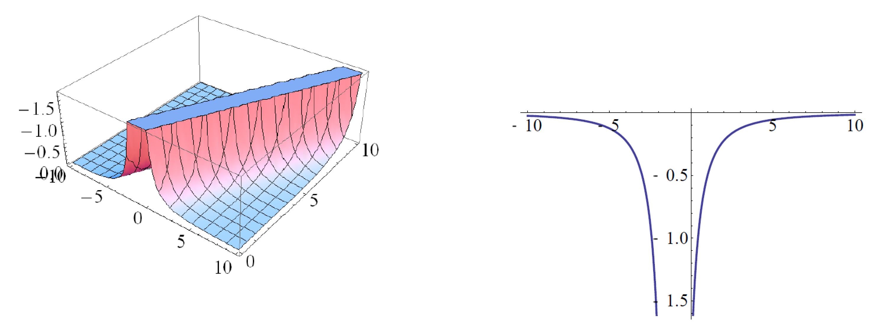
Figure 9.
The solutions (37) (a,b) and its projection when and . (c,d) shows the straddled solitary solution, which is a singular solution at .
Figure 9.
The solutions (37) (a,b) and its projection when and . (c,d) shows the straddled solitary solution, which is a singular solution at .

Figure 10.
The solutions (38) (a,b) and its projection when and (c,d) shows the singular solutions at .
Figure 10.
The solutions (38) (a,b) and its projection when and (c,d) shows the singular solutions at .
Publisher’s Note: MDPI stays neutral with regard to jurisdictional claims in published maps and institutional affiliations. |
© 2021 by the author. Licensee MDPI, Basel, Switzerland. This article is an open access article distributed under the terms and conditions of the Creative Commons Attribution (CC BY) license (https://creativecommons.org/licenses/by/4.0/).
Share and Cite
MDPI and ACS Style
Alotaibi, H. Traveling Wave Solutions to the Nonlinear Evolution Equation Using Expansion Method and Addendum to Kudryashov’s Method. Symmetry 2021, 13, 2126. https://doi.org/10.3390/sym13112126
AMA Style
Alotaibi H. Traveling Wave Solutions to the Nonlinear Evolution Equation Using Expansion Method and Addendum to Kudryashov’s Method. Symmetry. 2021; 13(11):2126. https://doi.org/10.3390/sym13112126
Chicago/Turabian StyleAlotaibi, Hammad. 2021. "Traveling Wave Solutions to the Nonlinear Evolution Equation Using Expansion Method and Addendum to Kudryashov’s Method" Symmetry 13, no. 11: 2126. https://doi.org/10.3390/sym13112126
Note that from the first issue of 2016, this journal uses article numbers instead of page numbers. See further details here.