Modified Combined-Step-Size Affine Projection Sign Algorithms for Robust Adaptive Filtering in Impulsive Interference Environments

Abstract

In this paper, to further improve the filtering performance and enhance the poor tracking capability of the conventional combined step-size affine projection sign algorithm (CSS-APSA) in system identification, we propose a simplified CSS-APSA (SCSS-APSA) by applying the first-order Taylor series expansion to the sigmoidal active function (of which the independent variable is symmetric) of CSS-APSA. SCSS-APSA has lower computational complexity, and can achieve comparable, or even better filtering performance than that of CSS-APSA. In addition, we propose a modification of the sigmoidal active function. The modified sigmoidal active function is a form of scaling transformation based on the conventional one. Applying the modified function to the CSS-APSA, we can obtain the modified CSS-APSA (MCSS-APSA). Moreover, the extra parameter of MCSS-APSA provides the power to accelerate the convergence rate of CSS-APSA. Following the simplification operations of SCSS-APSA, the computational complexity of MCSS-APSA can also be reduced. Therefore, we get the simplified MCSS-APSA (SMCSS-APSA). Simulation results demonstrate that our proposed algorithms are able to achieve a faster convergence speed in system identification.

1. Introduction

System identifications, including channel estimation, seismic system identification, noise or echo cancellation, and image recovery have been successfully realized by adaptive filters (AFs) [1]. Among conventional AF algorithms, the least-mean-square (LMS) and normalized LMS (NLMS) algorithms play important roles due to their low computational complexity and mathematical tractability [2,3]. However, such LMS-type algorithms suffer from filtering performance degradation under the heavy-tailed impulsive interference and heavy-colored input signal [4].

To remit the negative influence of heavy-colored input data on the convergence performance [5], derived the affine projection algorithm (APA), which is based on the idea of affine subspace projection. After that, the family of APA is developed by various methods [5,6,7,8,9,10,11,12,13,14,15,16]. Rather than a single current data vector used in LMS and NLMS, APA updates weight coefficients through multiple, most recent input vectors. Increasing the projection order of APA accelerates the convergence speed at the expense of computational complexity. However, APA is derived by the minimization of ${\ell }_2$-norm, which results in dramatic performance degradation under the non-Gaussian noise, especially for impulsive interference.

It is known that lower-order norms are robust against impulsive disturbances. From the perspective of computational simplicity, a great number of algorithms are derived by minimizing the ${\ell }_1$-norm to achieve robust filtering [10,17,18]. Moreover, [19] combined the AP method with ${\ell }_1$-norm optimization to derive a robust AP-like algorithm, which is termed the affine projection sign algorithm (APSA). To satisfy the contradictory requirements between fast convergence speed and small steady-state misalignment, the variable step-size APSA algorithms (VSS-APSAs) were proposed [20,21,22]. However, such VSS-APSAs reduce the tracking performance when the system abruptly changes. Therefore, to enhance the tracking performance of VSS-APSA, two convex combination methods are applied to APSA from different viewpoints. One is called the combination of APSA (CAPSA), and the other is named the combined step-size APSA (CSS-APSA). The CSS-APSA uses two different step sizes—the large one is related to faster convergence, and the small one is related to a lower steady-state misadjustment. In addition, the convex combination of affine projection-type algorithms using an impulsive noise indicator was developed [23]. However, [23] needs more calculations to realize good convergence performance. After that, the cost function based on the sigmodial active function was applied to a family of robust adaptive filtering algorithms, and it can be further simplified by the first-order Taylor series expansion [24].

In this paper, applying the first-order Taylor series expansion to the sigmodal active function (SAF) of CSS-APSA, we were inspired by [24] and will propose a simplified CSS-APSA (SCSS-APSA), which has lower computational complexity. However, although CSS-APSA realizes fast convergence rates and small steady-state misadjustment, there is still an open problem of enhancing convergence performance [25,26,27,28]. Therefore, we modify the formation of SAF in CSS-APSA. Using the modified SAF to improve the performance of traditional CSS-APSA, we propose a modified CSS-APSA (MCSS-APSA). In MCSS-APSA, the two different step sizes work in the same way as CSS-APSA; however, the extra parameter of modified SAF can enable flexible adjustment of filtering performance. In addition, similar operations of SCSS-APSA can also be used for MCSS-APSA, and then a simplified MCSS-APSA (SMCSS-APSA) can be derived. Simulation results demonstrate that the proposed algorithms can achieve good filtering performances in terms of the convergence speed in system identification.

The rest of this paper is organized as follows. Section 2 introduces the APSA algorithm based on step-size adjustment. In Section 3, after introducing the CSS-APSA algorithm, the proposal is derived. Section 4 lists the simulation results to demonstrate the effectiveness of proposed algorithms. Section 5 gives the conclusion.

2. Affine Projection Sign Algorithm Based on Step-size Adjustment

We review the traditional APSA and its variable step-size forms, which include the VSS-APSA [21] and CAPSA.

2.1. APSA

In the conventional APSA, the desired output signal is given by

$$d\left(n\right)={\mathbf{u}}^T\left(n\right){\mathbf{w}}^o+v\left(n\right),$$

(1)

where n is the time index; superscript T represents transposition of matrix or vector; ${\mathbf{w}}^o={[w_0^o,w_1^o,\dots ,w_{M-1}^o]}^T$ denotes an unknown system weight vector, which needs to be estimated; $\mathbf{u}\left(n\right)={[u\left(n\right),u(n-1),\dots ,u(n-M+1)]}^T$ is the input signal vector with length M; and $v\left(n\right)$ is the background noise with the addition of an interference signal.

Let $\mathbf{U}\left(n\right)$, $\mathbf{d}\left(n\right)$, $\mathbf{e}\left(n\right)$, and ${\mathbf{e}}_p\left(n\right)$ be the input matrix, desired signal vector, error vector, and a posteriori error vector, respectively, as follows:

$$\mathbf{U}\left(n\right)=\left[\mathbf{u}\right(n),\mathbf{u}(n-1),\dots ,\mathbf{u}(n-K+1\left)\right],$$

(2)

$$\mathbf{d}\left(n\right)={[d\left(n\right),d(n-1),\dots ,d(n-K+1)]}^T,$$

(3)

$$\mathbf{e}\left(n\right)=\mathbf{d}\left(n\right)-{\mathbf{U}}^T\left(n\right)\mathbf{w}(n-1),$$

(4)

$${\mathbf{e}}_p\left(n\right)=\mathbf{d}\left(n\right)-{\mathbf{U}}^T\left(n\right)\mathbf{w}\left(n\right),$$

(5)

where K is the affine projection order. The APSA algorithm can be derived by minimizing the ${\ell }_1$-norm of a posteriori error vector ${\mathbf{e}}_p\left(n\right)$ with a constraint on the filter coefficients, as

$$\begin{array}{c}\hfill \underset{\mathbf{w}\left(n\right)}{min}{\parallel \mathbf{d}\left(n\right)-{\mathbf{U}}^T\left(n\right)\mathbf{w}\left(n\right)\parallel }_1,\end{array}$$

(6)

$$\begin{array}{cc}\hfill \mathrm{subject}\mathrm{to}& {\parallel \mathbf{w}\left(n\right)-\mathbf{w}(n-1)\parallel }_2^2\le {\mu }^2,\hfill \end{array}$$

(7)

where ${\mu }^2$ is a parameter which is used to ensure the stability of the weight coefficients vector $\mathbf{w}\left(n\right)$ during updating. Using the method of Lagrange multipliers [19], the cost function can be solved by combining (6) and (7). Then, the updated equation for the weight vector is

$$\begin{array}{c}\hfill \mathbf{w}\left(n\right)=\mathbf{w}(n-1)+\mu \frac{{\mathbf{U}}_s(n-1)}{\sqrt{{\xi }_1+{\parallel {\mathbf{U}}_s(n-1)\parallel }_2^2}},\end{array}$$

(8)

where $\mu >0$ is the step size; $0<{\xi }_1\ll 1$ is to avoid division by zero; ${\parallel ·\parallel }_2$ is the ${\ell }_2$-norm of the vector; and ${\mathbf{U}}_s(n-1)=\mathbf{U}(n-1)\mathrm{sgn}\left(\mathbf{e}(n-1)\right)$ with $\mathrm{sgn}\left(\mathbf{e}\right(n-1\left)\right)$ being the sign operation on each element of the error vector.

2.2. VSS-APSA and CAPSA

A variable step size is based on the minimization of mean-square deviation [21], and given as follows:

$$\begin{array}{c}\hfill {\mu }_{vs}\left(n\right)={\alpha }_{vs}{\mu }_{vs}(n-1)+(1-{\alpha }_{vs})\times min(\frac{{\Vert \mathbf{e}\left(n\right)\Vert }_1}{\sqrt{\parallel {\mathbf{U}}_s{(n-1)\parallel }_2^2}},{\mu }_{vs}(n-1))\end{array}$$

(9)

where ${\alpha }_{vs}$ ($0<{\alpha }_{vs}<1$) is the smoothing factor. Although the VSS-APSA has good performance in terms of fast convergence speed and small steady-state misalignment, its tracking performance is very poor when an abrupt change occurs.

Therefore, to enhance the tracking performance of VSS-APSA, the convex combination method was applied to APSA (CAPSA). For APSA algorithms, two different step sizes, that is, ${\mu }_1>{\mu }_2>0$, are related to the faster convergence rate and lower steady-state error, respectively. The corresponding weight updates are defined as

$$\begin{array}{c}\hfill {\mathbf{w}}_1\left(n\right)={\mathbf{w}}_1(n-1)+{\mu }_1\frac{{\mathbf{U}}_s(n-1)}{\sqrt{{\xi }_1+{\parallel {\mathbf{U}}_s(n-1)\parallel }_2^2}},\end{array}$$

(10)

and

$$\begin{array}{c}\hfill {\mathbf{w}}_2\left(n\right)={\mathbf{w}}_2(n-1)+{\mu }_2\frac{{\mathbf{U}}_s(n-1)}{\sqrt{{\xi }_1+{\parallel {\mathbf{U}}_s(n-1)\parallel }_2^2}}.\end{array}$$

(11)

Combining ${\mathbf{w}}_1\left(n\right)$ with ${\mathbf{w}}_2\left(n\right)$ by a variable mixing factor $\lambda \left(n\right)\in [0,1]$ results in:

$$\begin{array}{c}\hfill \mathbf{w}\left(n\right)=\lambda \left(n\right){\mathbf{w}}_2\left(n\right)+(1-\lambda \left(n\right)){\mathbf{w}}_1\left(n\right).\end{array}$$

(12)

Generally, $\lambda \left(n\right)$ is updated indirectly based on reduction of an overall error $e\left(n\right)$ through a sigmoidal active function (SAF) [27,29], that is,

$$\begin{array}{c}\hfill \lambda \left(n\right)=\frac{1}{1+exp(-s(n\left)\right)},\end{array}$$

(13)

where $s\left(n\right)$ is based on a gradient descent scheme by using the ${\ell }_1$-norm minimization to ensure robustness in the presence of impulsive noise, as

$$\begin{array}{cc}\hfill s\left(n\right)& =s(n-1)-{\mu }_s\frac{\partial \mid e\left(n\right)\mid }{\partial s(n-1)}\hfill \\ \hfill & =s(n-1)+{\mu }_s{\mu }_{12}^{\lambda }\frac{{\mathbf{u}}^T\left(n\right){\mathbf{U}}_s(n-1)sgn\left(e\left(n\right)\right)}{\sqrt{{\xi }_1+{\parallel {\mathbf{U}}_s(n-1)\parallel }_2^2}},\hfill \end{array}$$

(14)

where ${\mu }_s>0$ is a step size, and ${\mu }_{12}^{\lambda }=({\mu }_2-{\mu }_1)[\lambda (n-1)(1-\lambda (n-1))+{\xi }_2]$, in which the factor ${\xi }_2$ is positive and prevents the update of $s\left(n\right)$ from halting when $\lambda (n-1)$ is equal to 1 or 0. Generally, $s\left(n\right)$ is restricted in a symmetric interval, that is, $[-4,4]$. (12) is the weight update of CAPSA when $s\left(n\right)<4$ and becomes $\mathbf{w}\left(n\right)={\alpha }_c{\mathbf{w}}_2\left(n\right)+(1-{\alpha }_c){\mathbf{w}}_1\left(n\right)+{\mu }_2\frac{{\mathbf{U}}_s(n-1)}{\sqrt{{\xi }_1+{\parallel {\mathbf{U}}_s(n-1)\parallel }_2^2}}$ only if $s\left(n\right)=4$. ${\alpha }_c(0\le {\alpha }_c\le 1)$ has the same meaning as ${\alpha }_{vs}$. However, from [25], we know that there is still an open problem to enhance the convergence performance of CAPSA.

3. Proposed Algorithms

We start by introducing the idea of the combined step-size APSA (CSS-APSA) algorithm. Then, we analyze the behavior of the mixing factor for CSS-APSA, and explain the reason why the mixing factor can be simplified. Finally, we derive the proposed algorithms.

In order to better identify the optimization problem, the cost functions need to be known. The CSS-APSA algorithm is derived by minimizing the ${\ell }_1$-norm of a posteriori error vector ${\mathbf{e}}_p\left(n\right)$ with a constraint on the filter coefficients, as

$$\begin{array}{c}\hfill \underset{\mathbf{w}\left(n\right)}{min}{\parallel \mathbf{d}\left(n\right)-{\mathbf{U}}^T\left(n\right)\mathbf{w}\left(n\right)\parallel }_1,\end{array}$$

(15)

$$\begin{array}{cc}\hfill \mathrm{subject}\mathrm{to}& {\parallel \mathbf{w}\left(n\right)-\mathbf{w}(n-1)\parallel }_2^2\le {\mu }_{12}^2,\hfill \end{array}$$

(16)

where

$$\begin{array}{c}\hfill {\mu }_{12}=\lambda \left(n\right){\mu }_2+(1-\lambda \left(n\right)){\mu }_1.\end{array}$$

(17)

Similar to the APSA [19], we can obtain the following:

For the SCSS-APSA:

$$\begin{array}{c}\hfill J_s\left(\mathbf{w}\left(n\right)\right)=\parallel \mathbf{d}\left(n\right)-{\mathbf{U}}^T{\left(n\right)\mathbf{w}\left(n\right)\parallel }_1{+\phi [\parallel \mathbf{w}\left(n\right)-\mathbf{w}(n-1)\parallel }_2^2-{\mu }_{s12}^2]\end{array}$$

(18)

For the MCSS-APSA:

$$\begin{array}{c}\hfill J_{\beta }\left(\mathbf{w}\left(n\right)\right)=\parallel \mathbf{d}\left(n\right)-{\mathbf{U}}^T{\left(n\right)\mathbf{w}\left(n\right)\parallel }_1{+\phi [\parallel \mathbf{w}\left(n\right)-\mathbf{w}(n-1)\parallel }_2^2-{\mu }_{\beta 12}^2]\end{array}$$

(19)

For the SMCSS-APSA:

$$\begin{array}{c}\hfill J_{s\beta }\left(\mathbf{w}\left(n\right)\right)=\parallel \mathbf{d}\left(n\right)-{\mathbf{U}}^T{\left(n\right)\mathbf{w}\left(n\right)\parallel }_1{+\phi [\parallel \mathbf{w}\left(n\right)-\mathbf{w}(n-1)\parallel }_2^2-{\mu }_{s\beta 12}^2]\end{array}$$

(20)

where $\phi$ is a Lagrange multiplier, ${\mu }_{s12}={\lambda }_s\left(n\right){\mu }_2+(1-{\lambda }_s\left(n\right)){\mu }_1$, ${\mu }_{\beta 12}={\lambda }_{\beta }\left(n\right){\mu }_2+(1-{\lambda }_{\beta }\left(n\right)){\mu }_1$, ${\mu }_{s\beta 12}={\lambda }_{s\beta }\left(n\right){\mu }_2+(1-{\lambda }_{s\beta }\left(n\right)){\mu }_1$, $J_s(·)$, $J_{\beta }(·)$, and $J_{s\beta }(·)$ represent the cost functions and discuss the computational complexity.

3.1. CSS-APSA

Substituting (10) and (11) into (12) yields the weight update of CSS-APSA (According to the symmetry, (12) can also be written as $\mathbf{w}\left(n\right)=\lambda \left(n\right){\mathbf{w}}_1\left(n\right)+(1-\lambda \left(n\right)){\mathbf{w}}_2\left(n\right)$ [25]) as

$$\begin{array}{cc}\hfill \mathbf{w}\left(n\right)& =\lambda \left(n\right){\mathbf{w}}_2\left(n\right)+(1-\lambda \left(n\right)){\mathbf{w}}_1\left(n\right)\hfill \\ \hfill & =\mathbf{w}(n-1)+[\lambda \left(n\right){\mu }_2+(1-\lambda \left(n\right)){\mu }_1]\hfill \\ \hfill & \times \frac{{\mathbf{U}}_s(n-1)}{\sqrt{{\xi }_1+{\parallel {\mathbf{U}}_s(n-1)\parallel }_2^2}}.\hfill \end{array}$$

(21)

3.2. Analysis of Variable Mixing Factors for CSS-APSA

Actually, the CSS-APSA algorithm uses the following SAF to adjust the mixing parameter

$$\begin{array}{c}\hfill \lambda \left(n\right)=\frac{C}{1+exp(-s(n\left)\right)}-\left(\frac{C}{2}-\frac{1}{2}\right),\end{array}$$

(22)

where $C>1$, and $s\left(n\right)$ is defined as

$$s\left(n\right)=\left\{\begin{array}{cc}-ln\left(\frac{C+1}{C-1}\right),\hfill & s\left(n\right)<-ln\left(\frac{C+1}{C-1}\right)\hfill \\ ln\left(\frac{C+1}{C-1}\right),\hfill & s\left(n\right)>ln\left(\frac{C+1}{C-1}\right)\hfill \\ s\left(n\right),\hfill & elsewhere.\hfill \end{array}\right.$$

(23)

According to (15), we can obtain

$$\begin{array}{c}\hfill \frac{\partial \lambda \left(n\right)}{\partial s\left(n\right)}=C\frac{exp(-s(n\left)\right)}{{(1+exp(-s\left(n\right)))}^2}.\end{array}$$

(24)

From (24), we know that $\lambda \left(n\right)$ is a monotone increasing function of $s\left(n\right)$. In other words, the increase rate of $\lambda \left(n\right)$ from 0 to 1 can be accelerated by increasing the value of C. Figure 1 shows the function curves of (22) and (23). From this figure, we know that $\lambda \left(n\right)$ is approximately equal to zero or one when $\left|s\right(n\left)\right|=0.3365$. Actually, the range of $s\left(n\right)$ is affected by two constraint conditions, namely, $s\left(n\right)\in [-4,4]$ and $\lambda \left(n\right)\in [0,1]$. Therefore, from (23) and such two constraints, we can obtain

$$\left\{\begin{array}{c}s\left(n\right)\in [s_{-},s_{+}]\hfill \\ s_{-}=max\left(-4,-ln\left(\frac{C+1}{C-1}\right)\right)\hfill \\ s_{+}=min\left(4,ln\left(\frac{C+1}{C-1}\right)\right)\hfill \end{array}\right..$$

(25)

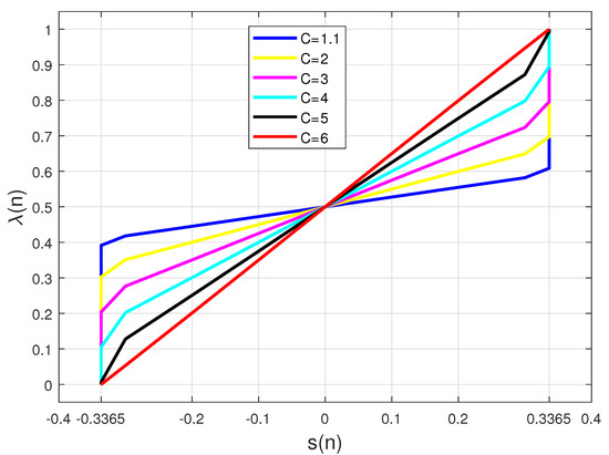
Figure 1. The curves of $\lambda \left(n\right)$ with different C values.

Furthermore, from (23) and (25), we know that:

• When the C value is small, such as $C=2$, we can get $s_{-}=-ln\left(\frac{2+1}{2-1}\right)=-1.0986$ and $s_{+}=1.0986$. When $\left|s\right(n\left)\right|=0.3365$, $\lambda \left(n\right)$ is approximately equal to 1 or 0. However, such two $\lambda \left(n\right)$ values will be slowly increased to 1 or decreased to 0 as $\left|s\right(n\left)\right|$ becomes larger. Therefore, the effective range for $s\left(n\right)$ can be treated as $[-0.3365,0.3365]$.
• From (23), as the C value becomes larger, $\left|s\right(n\left)\right|$ becomes closer to $0.3365$ because $ln\left(\frac{C+1}{C-1}\right)$ is a monotone decreasing function of C. Also, when the C value is relatively large, such as $C=6$, $\lambda \left(n\right)$ will be very close to 1 or 0. Therefore, for the large C value, we can constrain $s\left(n\right)\in [-0.3365,0.3365]$.

3.3. Practical Considerations about Proposed Algorithms

In this paper, to reduce the error of $\lambda \left(n\right)$ being 1 or 0, as shown in Figure 1 when $C\le 5$, we can appropriately extend the effective range of $s\left(n\right)$ to $[-0.4,0.4]$. In addition, when $s\left(n\right)=0.4$, the difference between $exp(-s(n\left)\right)$ and $1-s\left(n\right)$ is 0.0703. Ignoring such differences and applying the first-order Taylor series expansion to $exp(-s(n\left)\right)$, we can use $1-s\left(n\right)$ to approximate $exp(-s(n\left)\right)$. Hence, (22) can be simplified as

$$\begin{array}{c}\hfill {\lambda }_s\left(n\right)=\frac{C}{2-s\left(n\right)}-\left(\frac{C}{2}-\frac{1}{2}\right).\end{array}$$

(26)

Based on (26), we get

$$\left\{\begin{array}{c}s\left(n\right)=\frac{-2}{C-1}\to \lambda \left(n\right)=0\hfill \\ s\left(n\right)=\frac{2}{C+1}\to \lambda \left(n\right)=1.\hfill \end{array}\right.$$

(27)

Therefore, injecting (27) into (26) yields

$${\lambda }_s\left(n\right)=\left\{\begin{array}{cc}0,\hfill & s\left(n\right)<\frac{-2}{C-1}\hfill \\ 1,\hfill & s\left(n\right)>\frac{2}{C+1}\hfill \\ \frac{C}{2-s\left(n\right)}-(\frac{C}{2}-\frac{1}{2}),\hfill & elsewhere\hfill \end{array}\right.$$

(28)

with $C>1$. Also, applying (28) to CSS-APSA, we can get the simplified CSS-APSA (denoted as: SCSS-APSA).

Comparing (22) with (13), one can find that (22) is a kind of scaling transformation of (13). Such a transformation can speed up the change rate of $\lambda \left(n\right)$. Based on this idea, (22) can be modified as follows:

$$\begin{array}{c}\hfill {\lambda }_{\beta }\left(n\right)=\frac{C}{1+exp(-\beta s(n\left)\right)}-\left(\frac{C}{2}-\frac{1}{2}\right),\end{array}$$

(29)

where $\beta$ is a positive constant, and $s\left(n\right)$ is restricted as

$$s\left(n\right)=\left\{\begin{array}{cc}-ln\left(\frac{C+1}{C-1}\right)/\beta ,\hfill & s\left(n\right)<-ln\left(\frac{C+1}{C-1}\right)/\beta \hfill \\ ln\left(\frac{C+1}{C-1}\right)/\beta ,\hfill & s\left(n\right)>ln\left(\frac{C+1}{C-1}\right)/\beta \hfill \\ s\left(n\right)\hfill & elsewhere.\hfill \end{array}\right.$$

(30)

Following the modification of (29), different $\beta$ values can accelerate or slow down the change rate of ${\lambda }_{\beta }\left(n\right)$. The change rate may result in a faster convergence rate of the proposed algorithm. Therefore, CSS-APSA armed with (29) and (30) is called a modified CSS-APSA (denoted as MCSS-APSA).

Obviously, CSS-APSA is a special case of MCSS-APSA when the $\beta =1$. In addition to (29), when $C=1$, $s\left(n\right)$ is restricted as

$$s\left(n\right)=\left\{\begin{array}{cc}-4/\beta ,\hfill & s\left(n\right)<-4/\beta \hfill \\ 4/\beta ,\hfill & s\left(n\right)>4/\beta \hfill \\ s\left(n\right),\hfill & elsewhere.\hfill \end{array}\right.$$

(31)

Based on (16) and (23), the range of $\beta s\left(n\right)$ for MCSS-APSA is the same as that of $s\left(n\right)$ for CSS-APSA. Therefore, according to the operations for (26), when $C>1$ and $\beta >0$, (29) can also be simplified as

$$\begin{array}{c}\hfill {\lambda }_{s\beta }\left(n\right)=\frac{C}{2-\beta s\left(n\right)}-\left(\frac{C}{2}-\frac{1}{2}\right),\end{array}$$

(32)

and $s\left(n\right)$ is restricted as

$$s\left(n\right)=\left\{\begin{array}{cc}\frac{-2}{(C-1)\beta },\hfill & s\left(n\right)<\frac{-2}{(C-1)\beta }\hfill \\ \frac{2}{(C+1)\beta },\hfill & s\left(n\right)>\frac{2}{(C+1)\beta }\hfill \\ s\left(n\right),\hfill & elsewhere.\hfill \end{array}\right.$$

(33)

Therefore, injecting (32) and (33) into CSS-APSA, we can obtain the simplified MCSS-APSA (denoted as SMCSS-APSA). Algorithm 1 summarizes the proceeding of the proposed algorithms.

3.4. Computational Complexity

In Table 1, the computational complexity of the proposed SCSS-APSA, MCSS-APSA, and SMCSS-APSA are compared with that of APSA, CAPSA, and CSS-APSA in terms of the total number of additions, multiplications, comparisons, and exponents. It is clear that the simplified algorithms are more efficient in computation than CAPSA and CSS-APSA.

Table 1. Computational complexity of APSA, CAPSA, CSS-APSA, SCSS-APSA, MCSS-APSA, and SMCSS-APSA at each iteration.

Algorithms	Multiplications	Additions	Comparisons	Exponents
APSA	$2M(K+1)+1$	$M(2K+1)-1$	0	0
CAPSA	$2M(2K+3)+12$	$M(4K+4)+6$	2	0
CSS-APSA	$2M(K+1)+M+8$	$M(2K+2)+4$	2	2
SCSS-APSA	$2M(K+1)+M+8$	$M(2K+2)+4$	2	0
MCSS-APSA	$2M(K+1)+M+8$	$M(2K+2)+4$	2	2
SMCSS-APSA	$2M(K+1)+M+8$	$M(2K+2)+4$	2	0

Algorithm 1: The proposed Algorithms

Initialization:   $0<{\mu }_2<{\mu }_1$, $0<{\xi }_1\le 1$, $s\left(0\right)={\xi }_1$, $1<C$, $1\le \beta$, and ${\mathbf{w}}_1\left(0\right)={\mathbf{w}}_2\left(0\right)=\mathbf{0}$.   Computation:   while ${\{\mathbf{u}\left(n\right),d\left(n\right)\}}_{n\ge 1}$ available do    1: ${\mathbf{w}}_1\left(n\right)={\mathbf{w}}_1\left(n\right)+{\mu }_1\frac{{\mathbf{U}}_s(n-1)}{\sqrt{{\xi }_1+{\parallel {\mathbf{U}}_s(n-1)\parallel }_2^2}},$    2: ${\mathbf{w}}_2\left(n\right)={\mathbf{w}}_2\left(n\right)+{\mu }_2\frac{{\mathbf{U}}_s(n-1)}{\sqrt{{\xi }_1+{\parallel {\mathbf{U}}_s(n-1)\parallel }_2^2}},$    3: $\mathbf{w}\left(n\right)=\lambda \left(n\right){\mathbf{w}}_2\left(n\right)+(1-\lambda \left(n\right)){\mathbf{w}}_1\left(n\right),$    4: $e\left(n\right)=d\left(n\right)-{\mathbf{u}}^T\left(n\right)\mathbf{w}\left(n\right),$    5: $s\left(n\right)=s(n-1)-{\mu }_s\frac{\partial \mid e\left(n\right)\mid }{\partial s(n-1)},$    for SCSS-APSA    6: ${\lambda }_s\left(n\right)=\frac{C}{2-s\left(n\right)}-\left(\frac{C}{2}-\frac{1}{2}\right),$    7: if $s\left(n\right)<-ln\left(\frac{C+1}{C-1}\right)$:       then $s\left(n\right)=-ln\left(\frac{C+1}{C-1}\right)$,    8: else if $s\left(n\right)>ln\left(\frac{C+1}{C-1}\right)$:       then $s\left(n\right)=ln\left(\frac{C+1}{C-1}\right)$,    9: else $s\left(n\right)=s\left(n\right)$, end.    for MCSS-APSA    6: ${\lambda }_{\beta }\left(n\right)=\frac{C}{1+exp(-\beta s(n\left)\right)}-\left(\frac{C}{2}-\frac{1}{2}\right),$    7: if $s\left(n\right)<-ln\left(\frac{C+1}{C-1}\right)/\beta$:       then $s\left(n\right)=-ln\left(\frac{C+1}{C-1}\right)/\beta$,    8: else if $s\left(n\right)>ln\left(\frac{C+1}{C-1}\right)/\beta$:       then $s\left(n\right)=ln\left(\frac{C+1}{C-1}\right)/\beta$,    9: else $s\left(n\right)=s\left(n\right)$, end.    for SMCSS-APSA    6: ${\lambda }_{s\beta }\left(n\right)=\frac{C}{2-\beta s\left(n\right)}-\left(\frac{C}{2}-\frac{1}{2}\right),$    7: if $s\left(n\right)<\frac{-2}{(C-1)\beta }$:       then $s\left(n\right)=\frac{-2}{(C-1)\beta }$,    8: else if $s\left(n\right)>\frac{2}{(C+1)\beta }$:       then $s\left(n\right)=\frac{2}{(C+1)\beta }$,    9: else $s\left(n\right)=s\left(n\right)$, end.    end while

3.5. Steady-State Analysis

According to [24], the weight-error vector is defined as

$$\tilde{\mathbf{w}}\left(n\right)={\mathbf{w}}^o-\mathbf{w}\left(n\right).$$

(34)

Using (12), we can obtain:

$$\tilde{\mathbf{w}}\left(n\right)=\tilde{\mathbf{w}}(n-1)-{\mu }_{12}\frac{{\mathbf{U}}_s(n-1)}{\sqrt{\parallel {\mathbf{U}}_s{(n-1)\parallel }_2^2}}$$

(35)

$$\begin{array}{cc}\hfill \mathbb{E}[\parallel \tilde{\mathbf{w}}\left(n\right){\parallel }^2]& =\mathbb{E}[\parallel \tilde{\mathbf{w}}(n-1){\parallel }^2]-2{\mu }_{12}\mathbb{E}[{\tilde{\mathbf{w}}}^T(n-1)\frac{{\mathbf{U}}_s(n-1)}{\sqrt{\parallel {\mathbf{U}}_s{(n-1)\parallel }_2^2}}]\hfill \\ \hfill & +{\mu }_{12}^2\mathbb{E}[\frac{\parallel {\mathbf{U}}_s{(n-1)\parallel }^2}{\parallel {\mathbf{U}}_s{(n-1)\parallel }_2^2}],\hfill \end{array}$$

(36)

where $\mathbb{E}$ is the expectation operator. The mean-square-deviation $\mathbb{E}[\parallel \tilde{\mathbf{w}}\left(n\right){\parallel }^2]$ must be less than $\mathbb{E}[\parallel \tilde{\mathbf{w}}(n-1){\parallel }^2]$ to ensure the algorithm is stable, so the step-size ${\mu }_{12}$ must satisfy the following condition:

$$\begin{array}{c}\hfill 0<{\mu }_{12}<2\times \frac{\mathbb{E}\left[{\tilde{\mathbf{w}}}^T(n-1){\mathbf{U}}_s(n-1)\right]}{\mathbb{E}[\parallel {\mathbf{U}}_s(n-1){\parallel }^2/\sqrt{\parallel {\mathbf{U}}_s{(n-1)\parallel }_2^2}]}.\end{array}$$

(37)

For the SCSS-APSA, the step-size should satisfy the condition below:

$$\begin{array}{c}\hfill 0<{\mu }_{s12}={\lambda }_s\left(n\right){\mu }_2+(1-{\lambda }_s\left(n\right)){\mu }_1<2\times \frac{\mathbb{E}\left[{\tilde{\mathbf{w}}}^T(n-1){\mathbf{U}}_s(n-1)\right]}{\mathbb{E}[\parallel {\mathbf{U}}_s(n-1){\parallel }^2/\sqrt{\parallel {\mathbf{U}}_s{(n-1)\parallel }_2^2}]}.\end{array}$$

(38)

For the MCSS-APSA, the step-size should satisfy the condition below:

$$\begin{array}{c}\hfill 0<{\mu }_{\beta 12}={\lambda }_{\beta }\left(n\right){\mu }_2+(1-{\lambda }_{\beta }\left(n\right)){\mu }_1<2\times \frac{\mathbb{E}\left[{\tilde{\mathbf{w}}}^T(n-1){\mathbf{U}}_s(n-1)\right]}{\mathbb{E}[\parallel {\mathbf{U}}_s(n-1){\parallel }^2/\sqrt{\parallel {\mathbf{U}}_s{(n-1)\parallel }_2^2}]}.\end{array}$$

(39)

For the SMCSS-APSA, the step-size should satisfy the condition below:

$$\begin{array}{c}\hfill 0<{\mu }_{s\beta 12}=={\lambda }_{s\beta }\left(n\right){\mu }_2+(1-{\lambda }_{s\beta }\left(n\right)){\mu }_1<2\times \frac{\mathbb{E}\left[{\tilde{\mathbf{w}}}^T(n-1){\mathbf{U}}_s(n-1)\right]}{\mathbb{E}[\parallel {\mathbf{U}}_s(n-1){\parallel }^2/\sqrt{\parallel {\mathbf{U}}_s{(n-1)\parallel }_2^2}]}.\end{array}$$

(40)

In addition, $\lambda \left(n\right)=0$ in the transient state and $\lambda \left(n\right)=1(n\to \infty )$ in the steady state, such that ${\mu }_1$ or ${\mu }_2$, should also satisfy condition (36). Also, from [19], we know that $0<{\mu }_2,{\mu }_1\ll 1$, so the ranges of ${\mu }_{s12},{\mu }_{\beta 12}$, and ${\mu }_{s\beta 12}$ are restricted as

$$\begin{array}{c}\hfill 0<{\mu }_{s12},{\mu }_{\beta 12},{\mu }_{s\beta 12}\ll 1.\end{array}$$

(41)

4. Numerical Simulation Results

In this part, we test the filtering performance of the proposed algorithms in system identification. In this work, all simulation results have been averaged over 50 independent trials. The signal-to-noise ratio (SNR) was set to 30 dB, and background noise has been added to $d\left(n\right)$.

The impulsive noise $v\left(n\right)$ is modeled by $b\left(n\right)G\left(n\right)$, where $b\left(n\right)$ is a Bernoulli process with a probability of success of $P[b\left(n\right)=1]=p_r$, and $G\left(n\right)$ denotes zero-mean Gaussian noise with the variance ${\sigma }_G^2=1000{\sigma }_d^2$, where ${\sigma }_d^2$ is the average power of the desired output $d\left(n\right)={\mathbf{u}}^T\left(n\right){\mathbf{w}}^o$. We set ${\xi }_1={\xi }_2=0.001$, $K=2$, $p_r=0.1$, ${\mu }_1=0.01$, and ${\mu }_2=0.0001$ in all simulations. Following normalized MSD,

$$\mathrm{NMSD}=10{log}_{10}\left(\frac{\parallel {\mathbf{w}}^o{-\mathbf{w}\left(n\right)\parallel }_2}{\parallel {\mathbf{w}}^o{\parallel }_2}\right)$$

(42)

was used to measure the performance of the algorithms.

The color input datum were generated by filtering the white and zero-mean Gaussian signals with a unit power through a first-order system, as

$$\begin{array}{c}\hfill H_1=\frac{1}{1-0.7z^{-1}}.\end{array}$$

(43)

The unknown weight ${\mathbf{w}}^o$ was randomly generated with $M=32$ taps, and turned into $-{\mathbf{w}}^o$ at the middle of the iterations.

First of all, we investigated the influence of the parameter C on the performance of CSS-APSA. We chose $C\in \{1.1,2,3,4,5,6,7\}$, ${\mu }_s=1$. Figure 2 shows the corresponding NMSD curves. From this figure, we know that CSS-APSA with $C=5$ and $C=6$ can realize better filtering performance than that of other C values. In other words, proper C values can enhance the filtering performance of CSS-APSA. This result demonstrates the effectiveness of constraint on $s\left(n\right)\in [-0.3365,0.3365]$.

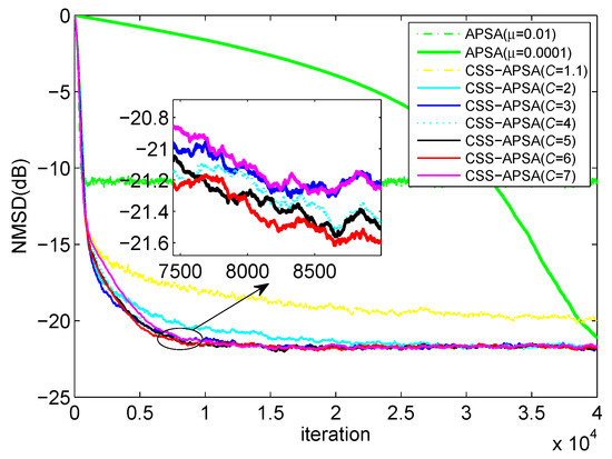
Figure 2. The NMSD curves of APSA and CSS-APSA with different C values.

Remark 1.

For CSS-type algorithms, when C is in a certain interval (such as $C\in (1,6]$), the performance of CSS-APSA can be improved by increasing the value of C. In addition, we can have following observations for $C\in (1,6]$:

• If the value of C is relatively small (such as $C\le 2$), the change rate of $\lambda \left(n\right)$ from 0 to 1 will be reduced. In this case, the combined algorithm has slower convergence speed. Figure 1 and Figure 2 illustrate such behavior.
• If the value of C is too large (such as $C=7$), the change rate of $\lambda \left(n\right)$ from 0 to 1 is increased in the process of iteration. In this case, $\lambda \left(n\right)$ tends to 1 too quickly, resulting in $\mathbf{w}\left(n\right)$ dominated by ${\mathbf{w}}_2\left(n\right)$, which is related to the lower steady-state error. Hence, the combined algorithm will still realize a slower convergence speed.

Secondly, we investigate the influence of ${\mu }_s$ on CSS-APSA with $C\in \{5,6\}$, since the ${\mu }_s$ as a step-size factor affects the update rate of $s\left(n\right)$ and indirectly influences the change rate of $\lambda \left(n\right)$. In this part, we set ${\mu }_s\in \{0.1,1,10\}$. Figure 3 plots the corresponding NMSD curves. From this figure, we know that ${\mu }_s=1$ is a better choice than other values. Hence, except where mentioned otherwise, we set ${\mu }_s=1$ in the following experiments. Furthermore, we compare the filtering performance between CSS-APSA and SCSS-APSA. Figure 4 plots the NMSD curves of the corresponding algorithms. Such results reveal that:

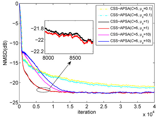
Figure 3. The NMSD curves of CSS-APSA with different ${\mu }_s$ values.

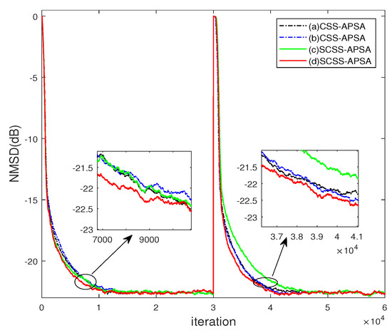
Figure 4. The NMSD learning curves of CSS-APSA and SCSS-APSA with different C. (a,c): $C=5$; (b,d): $C=6$.

• CSS-APSA with $C=6$ realizes faster convergence than $C=5$ after an abrupt change;
• SCSS-APSA with $C=6$ outperforms CSS-APSA in terms of convergence rate in the whole filtering process.

Moreover, Table 2 compares the execution times of CSS-APSA, SCSS-APSA, MCSS-APSA, and SMCSS-APSA at each iteration (computation platform: Intel(R) Core(TM) i7-4770K, CPU @ 3.50 GHz). One can clearly see that SCSS-APSA is more computationally efficient than CSS-APSA.

Table 2. Execution time of CSS-APSA, SCSS-APSA, MCSS-APSA, and SMCSS-APSA at each iteration.

Algorithms	Parameters	Execution Time (s)
CSS-APSA	$C=6$	1.7132
SCSS-APSA	$C=6$	1.6952
MCSS-APSA	$C=6,\beta =5$	1.7467
SMCSS-APSA	$C=6,\beta =5$	1.7108

Thirdly, we investigate the effect of parameter $\beta$ on the performance of MCSS-APSA. We set $C=6$ and $\beta \in \{1,5,10,20\}$. The NMSD curves are plotted in Figure 5, which shows that:

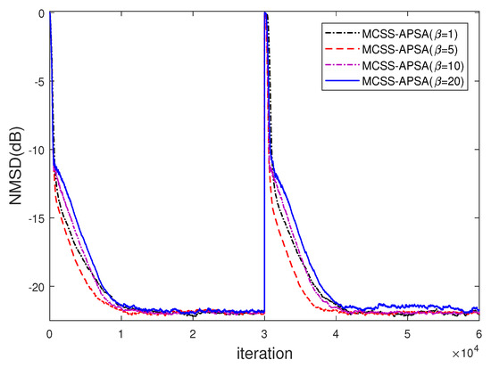
Figure 5. The NMSD curves of MCSS-APSA with different $\beta$, $C=6$.

• With $\beta =5$, MCSS-APSA realizes better filtering accuracy at a transient process than $\beta \in \{1,10,20\}$;
• With $\beta =1$, MCSS-APSA becomes to CSS-APSA, while MCSS-APSA with other $\beta$ values (such as $\beta =5$ or 10) outperforms CSS-APSA. This observation demonstrates the usefulness of modifications for CSS-APSA.
• Increasing the $\beta$ value from 1 to 20 cannot always improve the filtering performance of MCSS-APSA. Similarly to the effect of the C value, a $\beta$ value which is too large leads to $\mathbf{w}\left(n\right)$ dominated by ${\mathbf{w}}_2\left(n\right)$ in iterations, and slows down the convergence speed of MCSS-APSA.

Next, we compare the filtering performance between SMCSS-APSA and MCSS-APSA. In this part, we set $\beta =5$ and $C=6$, since such two parameters can improve the tracking performance of MCSS-APSA, as demonstrated in Figure 5. The compared NMSD results are plotted in Figure 6. From this figure, we can know that SMCSS-APSA achieves slightly better filtering behavior than that of MCSS-APSA, while the former is more computationally efficient than the latter, as demonstrated in Table 2.

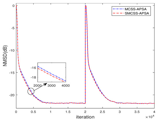
Figure 6. The NMSD curves of MCSS-APSA and SMCSS-APSA with $\beta =5$, $C=6$.

Finally, the filtering performance of SMCSS-APSA is compared with APSA, CAPSA, and SCSS-APSA (From [25], we know the VSS-APSA [21] need to reset algorithms when an abrupt change occurs, so we ignore the VSS-APSA’s comparison in system identification). Figure 7 shows the NMSD curves of these algorithms. The results demonstrate that SMCSS-APSA outperforms APSA, CAPSA, and SCSS-APSA in terms of the convergence rate.

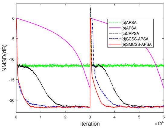
Figure 7. The NMSD learning curves of APSA, CAPSA, SCSS-APSA, and SMCSS-APSA with colored input data $H_1\left(z\right)$, (a): ${\mu }_1=0.01$; (b): ${\mu }_2=0.0001$; (c): ${\mu }_1=0.01$, ${\mu }_2=0.0001$; (d): $C=6$; (e): $C=6$, $\beta =5$.

5. Conclusions

In this paper, SCSS-APSA, MCSS-APSA, and SMCSS-APSA were derived to improve the convergence speed of CSS-APSA. To enhance the tracking performance of CAPSA and CSS-APSA, MCSS-APSA was proposed by using a modified sigmoidal active function. Furthermore, the simplification method was used on MCSS-APSA, resulting in SMCSS-APSA, which was found to achieve better filtering performance than that of MCSS-APSA. In addition, SCSS-APSA not only reduced the computational complexity of CSS-APSA, but also sped up the convergence under certain conditions. Simulations have shown that the proposed SCSS-APSA, MCSS-APSA, and SMCSS-APSA are superior to CSS-APSA.

References

- Guo, Y.; Li, J.; Li, Y. Diffusion correntropy subband adaptive filtering (SAF) algorithm over distributed smart dust networks. Symmetry 2019, 11, 1335. [Google Scholar] [CrossRef]
- Duttweiler, D.L. Proportionate normalized least-mean-squares adaptation in echo cancelers. IEEE Trans. Speech Audio Process. 2000, 8, 508–517. [Google Scholar] [CrossRef]
- Wang, Y.; Li, Y. Norm penalized joint-optimization NLMS algorithms for broadband sparse adaptive channel estimation. Symmetry 2017, 9, 133. [Google Scholar] [CrossRef]
- Min, S.; Nikias, C.L. Signal processing with fractional lower order moments: Stable processes and their applications. Proc. IEEE 1993, 81, 986–1010. [Google Scholar]
- Ozeki, K.; Umeda, T.; Members., R. An adaptive filtering algorithm using an orthogonal projecti on to an affine subspace and its properties. Electron. Commun. Jpn. 1984, 67, 126–132. [Google Scholar] [CrossRef]
- Shin, H.C.; Sayed, A.H.; Song, W.J. Variable step-size nlms and affine projection algorithms. IEEE Signal Process. Lett. 2004, 11, 132–135. [Google Scholar] [CrossRef]
- Lee, C.H.; Park, P. Optimal step-size affine projection algorithm. IEEE Signal Process. Lett. 2012, 19, 431–434. [Google Scholar] [CrossRef]
- Paul, T.K.; Ogunfunmi, T. On the convergence behavior of the affine projection algorithm for adaptive filters. IEEE Trans. Circuits Syst. Regul. Pap. 2011, 58, 1813–1826. [Google Scholar] [CrossRef]
- Yin, W.; Mehr, A.S. A variable regularization method for affine projection algorithm. IEEE Trans. Circuits Syst. Ii: Express Briefs 2010, 57, 476–480. [Google Scholar]
- Zhao, J.; Zhang, H.; Wang, G.; Liao, X. Modified memory-improved proportionate affine projection sign algorithm based on correntropy induced metric for sparse system identification. Electron. Lett. 2018, 54, 630–632. [Google Scholar] [CrossRef]
- Li, Y.; Jiang, Z.; Yin, J. Mixed norm constrained sparse apa algorithm for satellite and network echo channel estimation. IEEE Access 2018, 6, 65901–65908. [Google Scholar] [CrossRef]
- Sivabalan, S.R.A. Za-apa with zero attractor controller selection criterion for sparse system identification. Signal Image Video Process. 2018, 12, 371–377. [Google Scholar]
- Meng, R.; Lamare, R.C.D.; Nascimento, H. Sparsity-aware affine projection adaptive algorithms for system identification. In Proceedings of the Sensor Signal Processing for Defence (SSPD 2011), London, UK, 27–29 September 2011; pp. 27–29. [Google Scholar]
- Li, Y.; Zhang, C.; Wang, S. Low-complexity non-uniform penalized affine projection algorithm for sparse system identification. Circuits Syst. Signal Process. 2016, 35, 1611–1624. [Google Scholar] [CrossRef]
- Li, Y.; Li, W.; Yu, W.; Wan, J.; Li, Z. Sparse adaptive channel estimation based on lp-norm-penalized affine projection algorithm. Int. Antennas Propag. 2014, 2014, 17–23. [Google Scholar]
- Li, Y.; Hamamura, M. Smooth approximation l0-norm constrained affine projection algorithm and its applications in sparse channel estimation. Sci. World J. 2014, 2014, 937252. [Google Scholar]
- Arikan, O.; Cetin, A.E.; Erzin, E. Adaptive filtering for non-gaussian stable processes. IEEE Signal Process. Lett. 1994, 1, 163–165. [Google Scholar] [CrossRef]
- Kwong, C. Dual sign algorithm for adaptive filtering. IEEE Trans. Commun. 1986, 34, 1272–1275. [Google Scholar] [CrossRef]
- Shao, T.; Zheng, Y.R.; Member, S.; Benesty, J.; Member, S. An affine projection sign algorithm robust against impulsive interferences. IEEE Signal Process. Lett. 2010, 17, 327–330. [Google Scholar] [CrossRef]
- Yoo, J.; Shin, J.; Park, P. Variable step-size affine projection sign algorithm. IEEE Trans. Circuits Syst. II Express Briefs 2014, 61, 274–278. [Google Scholar]
- Shin, J.; Yoo, J.; Park, P. Variable step-size affine projection sign algorithm. Electron. Lett. 2012, 48, 9–10. [Google Scholar] [CrossRef]
- Zhang, S.; Zhang, J. Modified variable step-size affine projection sign algorithm. Electron. Lett. 2013, 49, 1264–1265. [Google Scholar] [CrossRef]
- Kim, S.H.; Jeong, J.J. Robust convex combination of affine projection-type algorithms using an impulsive noise indicator. Signal Process. 2016, 129, 33–37. [Google Scholar] [CrossRef]
- Huang, F.; Zhang, J.; Zhang, S. A family of robust adaptive filtering algorithms based on sigmoid cost. Signal Process. 2018, 149, 179–192. [Google Scholar] [CrossRef]
- Huang, F.; Zhang, J.; Zhang, S. Combined-step-size affine projection sign algorithm for robust adaptive filtering in impulsive interference environments. IEEE Trans. Circuits Syst. Express Briefs 2016, 63, 493–497. [Google Scholar] [CrossRef]
- Choi, J.H.; Cho, H.; Jeong, J.J.; Kim, W. Combination of step sizes for affine projection algorithm with variable mixing parameter. Electron. Lett. 2013, 49, 29–30. [Google Scholar] [CrossRef]
- Arenas-García, J.; Gómez-Verdejo, V. New algorithms for improved adaptive convex combination of lms transversal filters. IEEE Trans. Instrum. Meas. 2005, 54, 2239–2249. [Google Scholar] [CrossRef]
- Kozat, S.S.; Erdogan, A.T.; Singer, A.C.; Sayed, A.H. Steady-state mse performance analysis of mixture approaches to adaptive filtering. IEEE Trans. Signal Process. 2010, 58, 4050–4063. [Google Scholar] [CrossRef]
- Ferrer, M.; Gonzalez, A.; Member, S.; Diego, M.D. Convex combination filtered-x algorithms for active noise control systems. IEEE Trans. Audio Speech Lang. Process. 2013, 21, 156–167. [Google Scholar] [CrossRef]
© 2020 by the authors. Licensee MDPI, Basel, Switzerland. This article is an open access article distributed under the terms and conditions of the Creative Commons Attribution (CC BY) license (http://creativecommons.org/licenses/by/4.0/).