A New Model for Stock Management in Order to Rationalize Costs: ABC-FUCOM-Interval Rough CoCoSo Model
by
 , and
, and
Živko Erceg
1, 
Vitomir Starčević
2,
Dragan Pamučar
3,* ,
,
Goran Mitrović
4,
Željko Stević
1 and
and
Srđan Žikić
5 1
Faculty of Transport and Traffic Engineering, University of East Sarajevo, Vojvode Mišića 52, 74000 Doboj, Bosnia and Herzegovina
2
Faculty of Business Economics, University of East Sarajevo, Semberskih Ratara, 76300 Bijeljina, Bosnia and Herzegovina
3
Department of Logistics, Military academy, University of Defence in Belgrade, Pavla Jurisica Sturma 33, 11000 Belgrade, Serbia
4
Drina Insurance Company ad Milici, Bosnia and Herzegovina, Ulica 9. Januar broj 4, 75446 Milići, Bosnia and Herzegovina
5
Faculty of Management in Zajecar, Megatrend University, Belgrade, Park šuma Kraljevica, 19000 Zaječar, Serbia
*
Author to whom correspondence should be addressed.
Symmetry 2019, 11(12), 1527; https://doi.org/10.3390/sym11121527
Submission received: 3 December 2019
/
Revised: 12 December 2019
/
Accepted: 13 December 2019
/
Published: 17 December 2019
(This article belongs to the Special Issue Multi-Criteria Decision-Making Techniques for Improvement Sustainability Engineering Processes)
Abstract
:Cost rationalization has become imperative in every economic system in order to create adequate foundations for its efficient and sustainable management. Competitiveness in the global market is extremely high and it is challenging to manage business and logistics systems, especially with regards to financial parameters. It is necessary to rationalize costs in all activities and processes. The presence of inventories is inevitability in every logistics system, and it tends to create adequate and symmetrical policies for their efficient and sustainable management. In order to be able to do this, it is necessary to determine which products represent the largest percentage share in the value of procurement, and which are the most represented quantitatively. For this purpose, ABC analysis, which classifies products into three categories, is applied taking into account different constraints. The aim of this paper is to form a new model that involves the integration of ABC analysis, the Full Consistency Method (FUCOM), and a novel Interval Rough Combined Compromise Solution (CoCoSo) for stock management in the storage system. A new IRN Dombi weighted geometric averaging (IRNDWGA) operator is developed to aggregate the initial decision matrix. After grouping the products into three categories A, B and C, it is necessary to identify appropriate suppliers for each category in order to rationalize procurement costs. Financial, logistical, and quality parameters are taken into account. The FUCOM method has been used to determine the significance of these parameters. A new Interval CoCoSo approach is developed to determine the optimal suppliers for each product group. The results obtained have been modeled throughout a multi-phase sensitivity analysis.
1. Introduction
Managing all activities and processes, whether in engineering or any other area, requires proactive action and a focus on achieving sustainability. It primarily refers to the economic aspect of sustainability taking into account specific characteristics of an area in which certain research is conducted. Competitiveness in the market is huge and every company has to strive to reduce costs in its internal processes and activities since it is practically the only way to increase its competitiveness. This is also proved by Stojčić et al. [1] stating that in order to achieve a competitive market position, it is necessary to rationalize logistics activities and processes. A warehouse appears as one of the subsystems in which rationalization is possible and which, as a special logistics subsystem besides transportation, represents the biggest cause of logistical costs, and thus there is constant search for potential places for savings in these subsystems. One of the items that is certainly a problem for a large number of companies, whether referring to manufacture or distribution of finished products, is inventory. The goal is to find the optimal amount of inventory in order to control a warehouse in the best way possible and to rationalize the costs the logistics subsystem causes. This is mandatory if we want to achieve balance (symmetry) between production and consumption. For all the reasons given above, this paper examines the storage system from the aspect of stock management. Attention has to be directed towards performing all activities in the storage system in an efficient manner, which, in one way, is warehouse management as defined in [2]. The significance of this system and its management can be seen from the statement given in the above reference that warehouse systems and material handling are basic elements in the flows of goods and link manufacture and consumption points. It is for these reasons that it is important to establish an efficient synchronization of all activities and processes in the storage system, which is primarily achieved through adequate stock management.
This paper has several goals. The first goal relates to the development of a new approach that involves the Interval Rough Combined Compromise Solution (CoCoSo) model, which is a contribution to the literature that addresses multi-criteria models where uncertainty and imprecision exist. The integration of interval rough numbers and the CoCoSo method enables decision-makers to achieve more precise results based on their preferences. The second goal of the paper is to rationalize costs in the storage system through adequate stock management. It is primarily about identifying different groups of inventory and adopting adequate procurement policies. For this reason, in the subsequent phase, the selection of adequate suppliers for each group is performed. The third goal of the paper is to integrate the two aforementioned goals, which involves the creation of a new stock management model that combines different approaches: ABC analysis, the Full Consistency Method (FUCOM), and the Interval Rough CoCoSo model highlighting its benefits. It is important to note that such a model for stock management, which involves the integration of all the previous approaches, has not been noticed, and thus, from that aspect, the significance of this study can be perceived. With the formation of this model, the goal is to address efficiently one of typical warehouse planning issues, which is, according to Van den Berg and Zijm [3], warehouse management. In addition, it is necessary to achieve intelligent stock management that can result in reducing storage costs.
The rest of the paper is structured throughout several other sections. In the second section, a review of the literature related to the application of ABC analysis in inventory and stock management, and the application of multi-criteria decision-making (MCDM) methods in the storage system is presented. The third section presents a three-part methodology. The first part describes ABC analysis with certain constraints that have to be taken into account when executing it, while the second part is a brief overview of the FUCOM method. The third part in the third section presents the development of a new Interval Rough CoCoSo model with its algorithm given in detail. The fourth section is a case study presenting the problem in detail and the method to solve it. The fifth section includes an extensive sensitivity analysis using different models, as well as the discussion of the results obtained. Finally, there are concluding considerations with further research suggestions moving in several different directions. The algorithm of the developed IRN Dombi weighted geometric averaging (IRNDWGA) operator is provided in Appendix A.
2. Literature Review
ABC analysis is a frequently used technique to identify the state of stock management in a warehouse. Due to its simplicity on the one hand, and its great usefulness on the other, it has been noticed that it is widely used in various fields. The research conducted by Flores and Whybark [4] can be considered the first study that indicates the importance of applying multi-criteria optimization in the traditional ABC analysis. Flores and Whybark [5] supported the view through the advancement of their previous study by applying multi-criteria optimization in ABC analysis. Flores et al. [6] showed that the Analytic Hierarchy Process (AHP) method is one of the most appropriate multi-criteria techniques for stock classification in a warehouse. In their studies, Guvenir and Erel [7] and Malmborg et al. [8] went a step further and applied ABC analysis in combination with multi-criteria techniques and heuristic models (genetic algorithms). After these studies, Ramanathan [9] came up with the idea of optimizing storage systems using linear modeling (DEA model), combined with ABC analysis. That idea led to the comprehensive application of DEA and ABC analysis in evaluating the efficiency of storage systems.
ABC analysis was applied in [10] to control stock in a pharmaceutical company and create policies for managing it. Cycle counting calculations were performed and an inventory control application was based on the ABC-VED (vital, essential, desirable) model. Ishizaka et al. [11] applied the methodology to classify inventory into three groups based on three criteria: Annual Usage Value (AUV), Frequency Of Issue per year (FOI), and Current Stock Value (CSV). They formed the DEASort model that they applied with the Analytic Hierarchy Process (AHP) method. Compared to the single-criterion function, the study has concluded that the proposed model generates more savings per inventory classification groups. The study [12] also introduced a new hybrid model combining the ABC multi-criteria classification using the evolutionary algorithm with the MCDM method, the Technique for Order of Preference by Similarity to Ideal Solution (TOPSIS). The objective function of the model, as the authors point out, is to minimize inventory management costs, as well as to exploit the robustness and usefulness of partial approaches in the model, reduce the inventory costs, ensure acceptable performance, and meet the constraints of inventory management. It is concluded that the approach allows for more efficient inventory management. ABC analysis can certainly serve to create adequate policies to rationalize costs, as confirmed by the research [13] that created a new inventory management policy concerning the pre-existing situation that refers to spare parts. In order to increase the efficiency of inventory management and to solve the problem of single-criterion function, a hybrid approach, which involves ABC, AHP, and TOPSIS, is proposed in the research [14] for inventory management in an electronics company. Based on ABC analysis, in the study [15], the extraction of two spare parts requiring special treatment was performed, and the conditions for applying the Economic Order Quantity (EOQ) were obtained. Using the results of ABC analysis, a modification of the warehouse layout was made. The constant tendency to integrate different approaches with ABC analysis in order to create an adequate management model is also evident in the study [16] that has developed a new classification algorithm, called the FNS (functional, normal, and small) algorithm, which combines classical ABC classification with a new grouping strategy. In the algorithm, the handling frequency, lead time, contract manufacturing process, and specialty are used as input criteria, and the outputs are new classes for the inventories. The model has led to the result that inventories can be classified in more detail and useful management strategies can be created. For the purpose of inventory management regarding a Chinese manufacturer, the ELECTRE III method was combined with ABC analysis in the study [17]. It represents an innovative model for optimal classification of inventory. Ng [18] points out the lack of applying ABC analysis alone because, as already noted, it is based on only single criterion. Therefore, in his paper, in which he also emphasizes the importance of other criteria, he has developed a simple model for multiple criteria inventory classification. The model converts all criteria measures of an inventory item into a scalar score. The classification based on the calculated scores using ABC principle is applied. Various approaches have been developed to create adequate foundations for inventory optimization in storage systems, as already been emphasized. It is important to note that the study [19] combined rough set theory with ABC analysis by considering additional criteria.
In addition to crisp multi-criteria decision-making (MCDM) techniques, the authors applied a fuzzy technique to include uncertainties when evaluating storage systems. Thus, fuzzy AHP was applied to evaluate the hydrogen storage system in the automotive industry [20]. To improve supply chain performance, companies need to select an adequate warehouse location that will meet multiple needs and requirements. The combination of fuzzy AHP and fuzzy TOPSIS was applied in [21] for the optimal selection of five potential warehouse locations. The importance and impact of warehousing on the complete efficiency of supply chains has been confirmed in a number of studies, such as [22,23,24,25]. Ashrafzadeh et al. [22] point out that the selection of a warehouse location is of strategic importance for many companies. In the study, the fuzzy TOPSIS method was used to evaluate potential warehouse locations. The study [25] is noticeable in the area of the supply chain management of hazardous substances. The study shows the influence of selecting an appropriate warehouse location on reducing the risk of negative effects. In the study, the authors use the fuzzy Multi-Objective Optimization Ratio Analysis (MULTIMOORA) technique for multi-criteria optimization of warehouse locations. The combination of MCDM methods in integration with fuzzy logic was also applied in [23] to determine a warehouse location. In the study, the authors used fuzzy TOPSIS, fuzzy Simple Additive Weighting (SAW), and fuzzy Multi-Objective Optimization Ratio Analysis (MOORA) methods, while Emeç and Akkaya [26] applied stochastic AHP and VlseKriterijumska Optimizacija I Kompromisno Resenje (VIKOR) for the same purpose.
Fuzzy multi-criteria decision-making is also used for other tasks related to storage systems. Saputro and Daneshvar Rouyendegh [27] evaluated and selected material handling equipment in a warehouse using a hybrid multi-criteria model that involves the use of fuzzy AHP and fuzzy TOPSIS techniques. In their study, Erkan and Can [28] demonstrated the importance of using barcode technology, i.e., Radio Frequency Identification (RFID) technology to optimize logistics processes. For that purpose, they applied the fuzzy AHP method.
3. Methods
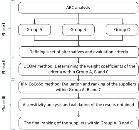
This paper introduces a new methodology for stock management in the storage system with the aim of rationalizing costs and creating an adequate stock management model (Figure 1). The proposed methodology is implemented throughout three phases. In the first phase, on the basis of procurement costs, the classification of inventory in the storage system is performed using ABC analysis. After grouping the products into Groups A, B, and C, product ordering policies and the time interval for controlling the products are defined. After defining the groups, potential suppliers (different number of suppliers) for each of these groups are considered, i.e., those who are specialized in specific types of products. In this way, the second phase is approached defining the criteria for selecting suppliers and potential alternatives for each group individually. In this phase, the application of FUCOM defines the weight coefficients of the criteria within each of Groups A, B, and C. In the third phase, expert evaluation of alternatives and aggregation of expert decisions into a single decision matrix are conducted. The uncertainties and inaccuracies in expressing expert preferences are represented by the use of interval rough numbers (IRN). The evaluation of alternatives is conducted using the Interval Rough (IR) CoCoSo model. As a result of the IR CoCoSo model, a ranking of suppliers is obtained within each Group, A, B, and C. In the next step, validation of the obtained results and making the final decision are carried out within a sensitivity analysis of the results.
In addition to the model being described in detail, it is important to highlight again the completely new elements of the model: The Interval Rough (IR) Combined Compromise Solution (CoCoSo) model and the IRN Dombi weighted geometric averaging (IRNDWGA) operator.
3.1. ABC Analysis
One of the most frequently used inventory classification techniques is ABC analysis [9,14]. During the last decades, many companies have taken seriously the task of managing the inventory efficiently because of the surplus of stock and the need to make more profits for their financial and logistical well-being. For this purpose, the ABC classification is one of the most frequently used analyses in production and inventory management domains, in order to classify a set of items in the three predefined classes A, B, and C, where each class follows a specific management and control policies [12]. Efficient inventory classification is a vital activity for companies that handle large quantities of inventory.
Considering all of the above, it can be concluded that ABC analysis is, in one way, indispensable in the creation of inventory management models, but not sufficient. This is confirmed by the study [14] stating that ABC analysis is one of the most frequently used inventory classification techniques, but this technique considers only a single criterion as the annual sales volume of each item. Therefore, different approaches are developed depending on a case study in which different techniques are integrated, as is the case in this paper.
ABC analysis is a stochastic method. It is very simple, and that is the reason why it is widely used in the field of material and commodity business. ABC analysis aims to maximize cost-effectiveness and productivity and increase business success and economy. It is used in companies that have a wide range of products. The purpose of using this analysis is to establish a functional control and management system within the procurement and warehousing business, and thus the possibility of achieving greater cost-effectiveness of the company. ABC analysis is based on the most important products that are of greatest benefit, i.e., they bring in the most revenue. The process of conducting ABC analysis can be described in three phases. The first phase is collecting data on annual requirements or material consumption by types over a certain period, usually one year. After that, the values of requirements/consumption are calculated by multiplying the quantities of individual materials by their planned or average purchase prices. Then, the materials are sorted in descending order by the values of annual requirements/consumption, the percentage share of the value of individual materials in the total value of annual requirements/consumption is calculated and the percentage shares are cumulated. A comparison of the cumulative percentages of the annual requirements/consumption and the percentages of the number of types is performed to determine Groups A, B, and C, and for each product the group it belongs to.
The cost share of the total procurement value should comply with the constraint represented by Equation (1).
The share in the total number (quantity) of different types of products should comply with the constraint represented by Equation (2).
The third constraint implies that there are most products of C, followed by B and least products of A, which is shown in Equation (3).
3.2. Full Consistency Method FUCOM
One of the new methods that is based on the principles of pairwise comparison and validation of results through deviation from maximum consistency is the full consistency method (FUCOM) [29]. Benefits that are determinative for the application of FUCOM are a small number of pairwise comparisons of criteria (only n−1 comparison), the ability to validate the results by defining the deviation from maximum consistency (DMC) of comparison, and appreciating transitivity in pairwise comparisons of criteria. The FUCOM model also has a subjective influence of a decision-maker on the final values of the weights of criteria. This particularly refers to the first and second steps of FUCOM in which decision-makers rank the criteria according to their personal preferences and perform pairwise comparisons of ranked criteria. However, unlike other subjective models, FUCOM has shown minor deviations in the obtained values of the weights of criteria from optimal values [29,30,31,32,33]. Additionally, the methodological procedure of FUCOM eliminates the problem of redundancy of pairwise comparisons of criteria, which exists in some subjective models for determining the weights of criteria.
Assume that there are n evaluation criteria in a multi-criteria model that are designated as wj, j = 1, 2,..., n, and that their weight coefficients need to be determined. Subjective models for determining weights based on pairwise comparison of criteria require a decision-maker to determine the degree of impact of the criterion i on the criterion j. In accordance with the defined settings, Figure 2 presents the FUCOM algorithm [34].
3.3. A New MCDM Model—Interval Rough CoCoSo Approach
The process of group decision-making is accompanied by a great amount of uncertainty and subjectivity, so decision-makers often have dilemmas when assigning certain values to decision attributes [34]. Suppose that one decision attribute should be assigned a value presented by a qualitative scale whose values range from 1 to 7. One decision-maker (DM) may consider that the decision attribute should have a value between 5 and 6, another DM may consider that a value between 4 and 5 should be assigned, while the third DM has no dilemma about the value of the decision attribute and assigns a value of 5. The dilemmas presented are extremely common in a group decision-making process. In such situations, one of the solutions is to geometrically average two values between which individual decision-makers are in doubt. However, in such situations, the uncertainty (ambiguity) that prevailed in a decision-making process would be lost and further calculation would be reduced to crisp values. On the other hand, the use of fuzzy [35,36] or grey techniques would entail predicting the existence of uncertainty and subjectively defining the interval by which uncertainty is exploited. Subjectively defined intervals in further data processing can significantly influence the final decision, which should definitely be avoided if we aim at impartial decision-making. On the contrary, the approach based on interval rough numbers includes exploiting the uncertainty that exists in the data obtained [34].
In this paper, a new approach in the theory of rough sets, a CoCoSo approach based on Interval Rough Numbers (IRN), is proposed to process the uncertainty contained in data in group decision-making. The crisp CoCoSo method was developed in 2018 by Yazdani et al. [37].
The Interval Rough CoCoSo approach consists of seven steps, which are explained below.
Step 1. Forming the initial decision-making matrix (X).
In the first step, it is needed to perform the evaluation of alternatives by criteria. The procedure for obtaining the basic decision-making matrix (X) is the same as in other MCDM approaches. In this approach interval rough numbers are applied as input parameters. Advantages of application Interval Rough Numbers (IRN) are presented in [34].
Based on Equations (1)–(13) from [34], we determine the vectors , where represents the value of alternative by criteria ( ).
where represents the number of alternatives, represents the number of criteria. The initial (aggregated) decision matrix can be obtained using some of IRN operators.
Step 2. Normalization of the initial interval rough group matrix using Equations (5)–(9)
where represents the elements of the interval rough normalized matrix ().
(a) For “benefit type” criteria (maximum value of criteria is preferable)
(b) For “cost type” criteria (minimum value of criteria is preferable)
where and represent the minimum and maximum values of the rough boundary interval of the observed criteria, respectively:
Step 3: Weighting the previous normalized interval rough matrix using Equation (10):
represents the weight coefficients of criteria.
Step 4: Summing all the values of the alternatives obtained (summing by rows) using Equation (11):
Step 5. Determination of the weighted sum model using Equations (12) and (13):
Step 6. Determination of aggregated strategies.
In this step, three aggregated appraisal scores are used to generate relative performance scores of the alternatives, using Equations (14)–(17):
First, it is required to calculate the sum of matrices and . In this way, the matrix is obtained by applying Equation (14)
Subsequently, all values by columns are summed and the matrix is obtained.
Equation (15) represents the arithmetic mean of sums of and scores, while Equation (16) signifies the sum of relative scores of and . Equation (17) computes a balanced compromise score of and models. In Equation (17), the value of λ ranges from 0 to 1 and can be chosen by the decision-maker.
Step 7: The final ranking of the alternatives is determined based on ki values:
Higher ki values indicate better position of the alternatives in the ranking pre-order.
The ranking of alternatives is performed by transformation of the interval rough numbers into real numbers , applying Equations (19) and (20) from [38].
where and represents the rough boundary intervals of .
4. Case Study
The proposed model, which is shown and explained in detail in Figure 1, was implemented in a company engaged in trading activities and its own production of building materials. It is located in the territory of Bosnia and Herzegovina. It is important to note that in the recent past, the company has also introduced the production of eco-pellets, which indicates that it is trying to take care of sustainability aspects as well.
4.1. Application of ABC Analysis for Product Classification
The input parameters for ABC analysis are the parameters obtained from the procurement report at the retail facility of the company where the research was conducted. The data collected cover one calendar year, i.e., the complete period of the previous year. Product characteristics are systematized by: Product code, product name, quantity of products purchased, purchase value per unit of product, and total value of procurement. Based on the financial parameters, ABC analysis has been carried out, part of which is shown in Table 1. The product assortment for the observed annual period is a total of 83 products.
After ABC analysis, complying with the constraints presented by Equations (1)–(3), the results given in Figure 3 are obtained.
Figure 3 shows the number of products per groups, the percentage share of the number of products, and the percentage share of the costs. Based on the results obtained, the following can be observed. Group A consists of eight products, i.e., 9.6% of the total number of products, which certainly represents the smallest number of classified groups, but with the highest value. Therefore, these products represent a total of 75.3% of procurement costs since they are products with higher value or higher demand. There are 26 products classified in Group B, which is 31.3% of the total number of products. In respect of financial structure, i.e., the costs of this product category, they are 19.5%, while Group C products account for 5.12% of the cost structure but represent the largest part of the products in percentage and numerical terms; 59% and 49%, respectively. Group A consists of products that are of highest priority for the company. There is a high need for these products, and they have a high value, so they need special attention. It is reflected in more frequent and rigorous control, thorough preparation of procurement activities and the creation of partnerships with potential suppliers. Considering the products that belong to Group B, it is necessary to pay almost as much attention as to the previous group, with some minor changes. This group of products needs to be controlled less frequently; two to three times a year. Group C includes the large number in the total number of products, but they are of very low values. For this group of products, the procurement processes should be simplified as much as possible and higher amount of security stock should be kept. Most commonly, the orders cover the annual requirements, so the control mostly takes place once a year.
4.2. Calculation of the Criterion Weights Applying the FUCOM Method
The criteria used to evaluate the suppliers within each group are: C1—Payment method (max), C2—Financial stability (max), C3—Product price (min), C4—Delivery time (min), C5—Reliability (max), C6—Flexibility (max), C7—Product quality (max), C8—Warranty period (max) and C9—Reputation (max). Three of these criteria belong to financial criteria, logistic parameters, and quality indicators, respectively. After performing the calculation and applying all the steps of the FUCOM method, the vectors of weight coefficients within each of the groups are defined, as shown in Figure 4.
Figure 4 shows the values of all the criteria for suppliers to be evaluated within the three groups. Considering the results of ABC analysis and the types of products belonging to different groups, the results are as follows:
- -
- Group A: ;
- -
- Group B: ; and
- -
- Group C: .
4.3. Evaluation of Suppliers Applying the Interval Rough CoCoSo Model
The final values of the weight coefficients obtained by the FUCOM model are further used to evaluate and select the optimal alternative (supplier) in the IR CoCoSo multi-criteria model. The evaluation of suppliers is performed within the three groups defined in ABC analysis. Eight suppliers are evaluated in Group A, six suppliers are considered in Group B, while nine suppliers are analyzed in Group C. The suppliers are evaluated within each group on the basis of the nine criteria previously presented. Applying the IR CoCoSo model within each group, a rank of suppliers is defined. The alternatives are evaluated using the linguistic scale: Very good (VG), 9; Good (G), 7; Medium (M), 5; Fair (F), 3; and Poor (P), 1.
In the research, three experts took part and evaluated the suppliers using the predefined scale. Thus, three correspondent expert matrices were obtained within each group of suppliers, one for each expert, respectively (Table 2).
Step 1. The initial (aggregated) decision matrix (Table 3) is obtained using the IRN Dombi weighted geometric averaging (IRNDWGA) operator, Equation (A2). IRNDWGA is derived from the rough Dombi weighted geometric averaging operator presented in [39] and given in Appendix A.
Applying Equation (A2), the experts’ individual IRN matrices are transformed into an aggregated IRN initial decision matrix. Thus, e.g., at position A1-C1 (Supplier Group A), the following values in expert correspondent matrices are obtained:
, and . As mentioned in the previous part of the paper, three experts participated in the study and were assigned the following weight coefficients . Based on the values shown in Equation (A2) and assuming that is at position A1-C1, the aggregation of values is performed, as follows:
Thus, at position A1-C1, a rough aggregated value is obtained applying the IRNDWGA operator (Table 3). The aggregation of the residual values from Table 3 is performed (using Equation (A2)) in a similar way.
Step 2: In this step, using Equations (6) and (7), the initial decision matrix is modified, and a normalized matrix is formed (Table 4).
An example of normalization for benefit criteria is explained for for Group A:
An example of normalization for cost criteria is explained for for Group A:
Step 3: In this step, Equation (10) is applied in order to perform the weighting of the previously obtained matrix with the criterion values identified by using the FUCOM method. An example of the calculation of this matrix shown in Table 5 is as follows:
Step 4 and 5. The following section presents the weighted IR sequences, and , which are further used to compare the alternatives. The sequences and are obtained using Equations (11)–(13) and are shown in Table 6.
The sequence for the first alternative for Group A is obtained as follows:
The sequence for the first alternative for Group A is obtained as follows:
Step 6: Applying Equations (14)–(17), the relative significance of the alternatives is obtained within the aggregation strategies. When calculating the relative significance of alternatives within the third aggregation strategy, the value of the coefficient λ is taken as 0.5. The effect of changing the coefficient λ () on the change in the relative significance of alternatives has been considered in the discussion of the results. The relative significance of the alternatives within the integration strategies, as well as the final ranking of alternatives by Groups A, B, and C, is shown in Table 7.
First, it is required to calculate the sum of matrices and . In this way, the matrix is obtained by applying Equation (14).
An example of the calculation is as follows:
Subsequently, all values by columns are summed and a matrix is obtained:
Applying Equation (15), the first aggregation strategy is obtained:
Applying Equation (16), the second aggregation strategy is obtained:
Applying Equation (17), the third aggregation strategy is obtained:
First, the following matrix is calculated:
whose elements are obtained as follows:
After that, the following matrix is calculated:
and is obtained as follows:
Step 7. The final ranking of the alternatives is obtained by applying Equation (18).
The alternatives are ranked based on the value of k, whereby it is preferable that the alternative has a value of k as high as possible. Based on the values obtained, it can be concluded that the initial ranking of suppliers using the FUCOM-IR CoCoSo model is; Group A: A3 > A2 > A5 > A6 > A4 > A8 > A7 > A1, Group B: A2 > A4 > A5 > A3 > A6 > A1, and Group C: A7 > A2 > A1 > A3 > A4 > A9 > A8 > A5 > A6.
5. Validation of the Results through Sensitivity Analysis
In the following part, the results presented in the previous section are validated through sensitivity analysis. Validation was performed throughout three phases. In the first phase, the impact of changing the parameters λ and ρ on the ranking results was analyzed. In the second phase, the impact of changing the most significant criterion on the ranking results was performed. In the third phase, the results of the FUCOM-IRN CoCoSo model were compared with the results of other multi-criteria techniques.
In the earlier research [39], it is shown that changes in the parameter ρ lead to the transformation of Dombi functions, and thus to the change in the values of the functions. The impact of the parameters ρ on the results of the functions can be significant. It is therefore a logical step to check the impact of the parameters ρ on the final ranking results when validating the results. An analysis of the change in the value of the parameter ρ was performed throughout a total of 100 scenarios, where the change of the parameter ρ was analyzed in the interval . The change in the parameter ρ in the interval was analyzed in each of the considered groups of suppliers (Group A, B, and C). The results of the impact of the parameter ρ on changes in the values of the criterion functions of alternatives are shown in Figure 5.
Generally, increasing the value of the parameter ρ, the process of calculating the IRN Dombi functions is becoming more complex. Decision-makers most often choose the value of this parameter in accordance with their preferences. When making decisions in real systems and in real time, it is recommended that value one is taken for the value of ρ. The parameter value ρ = 1 simplifies the decision-making process. Figure 5 shows that when the parameter ρ has different values, the ranking positions of the considered alternatives in Group B remain the same. In Group A, the parameter values of the sixth-ranked and seventh-ranked alternatives (A7 and A8) have swapped places, while, for the remaining values of the parameter ρ, the initial ranking from Table 7 has been confirmed. At the same time, the rankings of the remaining alternatives are unchanged. It is similar in Group C of suppliers. For parameter values ρ > 1, the fourth-ranked and fifth-ranked alternatives (A1 and A4) have swapped places, while the rankings of the remaining alternatives are unchanged. This means that there is a satisfactory advantage between the most influential alternatives and that the alternatives A3 and A2 (Group A), A2 and A4 (Group B), and A7 and A2 (Group C) stand out as dominant in the considered set. Thus, changes in the value of the parameter ρ have an impact on the change in the value of the criterion functions of the alternatives, but these changes are insufficient to cause major changes in the ranks.
In the following part, the impact of changing the parameter λ on the rankings of alternatives is discussed. Throughout 100 scenarios, the analysis of the impact of the coefficient λ value on the change of the criterion functions and the rankings of the alternatives have been analyzed. In the initial scenario (S1), the value of λ = 0.01 has been considered. In each subsequent scenario, the value of λ is increased by the value of 0.01. Thus, a total of 100 scenarios have been formed. The results show that the parameter λ does not affect changes in the value of the criterion functions, and nor the supplier ranks. It should be emphasized that this only applies to the example discussed in this paper. For other values of the alternatives in the initial decision matrix, the impact of the parameter λ may influence the change in the result. Therefore, such an analysis should be an indispensable step in checking the stability of proposed ranks.
In the second phase of result validation, i.e., sensitivity analysis, an analysis of the impact of changing the most significant criterion (C1) on the ranking results by supplier groups has been performed. Based on the recommendations given in [40,41,42], a total of 20 scenarios are formed applying Equation (21), [41].
where represents the corrected value of criteria C2–C9, represents the impaired value of the C1 criterion, represents the original value of the considered criterion, and represents the original value of the C1 criterion.
In the first scenario, the value of the C1 criterion was reduced by 2%, while the values of the remaining criteria were proportionally corrected using Equation (21). In each subsequent scenario, the value of the C1 criterion was reduced by 5% while the values of the remaining criteria were adjusted to meet the condition . After the formation of new 20 vectors of the weight coefficients of the criteria for each supplier group, new supplier ranks were obtained (Figure 6).
Analyzing the data from sensitivity analysis (Figure 6), we can conclude the following:
- (1)
- Group A: Changes in the values of the most significant criterion C1 lead to the changes in the ranks of alternatives A1, A2, A4, A6, A7, and A8. The first-ranked alternative A3 and the fourth-ranked alternative A5 have maintained their positions across all 20 scenarios. Thus, we can conclude that the alternative A3 stands out as the best and has a sufficient advantage over the remaining alternatives. In addition, rank correlation analysis using Spearman’s correlation coefficient has confirmed that the rank changes of the above alternatives are minimal since the average value of the Group A correlation coefficient is 0.88. This value of the correlation coefficient shows that there is a high correlation of the obtained ranks with the initial rank from Table 3, i.e., the changes in the ranks are minimal. Thus, we can conclude that the rank obtained is confirmed and credible.
- (2)
- Group B: From Figure 6, we can see that changes in the value of criterion C1 lead to a change in the rank of the fourth-ranked and fifth-ranked alternatives, A3 and A6. The remaining alternatives have maintained their positions throughout all 20 scenarios. This shows us that alternatives A2 and A4 stand out as the best alternatives that have a sufficient advantage over the other alternatives. As with Group A, there is a high rank correlation here as well, which is confirmed by the mean of correlation coefficient in Group B (Group B = 0.97) which is extremely high.
- (3)
- Group C: Changes in the values of the C1 criterion in 20 scenarios lead to a change in the ranks of alternatives A2, A1, A3, and A4. At the same time, the remaining alternatives A7, A9, A8, A5, and A6 have maintained their rankings across all 20 scenarios. The best-ranked alternative A7 has remained the best-ranked alternative in all 20 scenarios, and we can conclude that the A7 alternative has a sufficient advantage over the remaining alternatives. The Spearman’s correlation coefficient (Group C = 0.91) shows that there is a high correlation between the obtained ranks and the initial rank from Table 7, which leads us to the conclusion that the rank obtained is confirmed and credible.
In the third phase, the rankings of the IRN CoCoSo models were compared with the results of other multi-criteria techniques: IRN WASPAS [43,44], IRN MABAC [43], and IRN MAIRCA [41]. The results of the ranking when applying the above multi-criteria techniques are shown in Figure 7.
The ranking results show that all multi-criteria models for Group B and Group C confirm the rankings of the first-ranked alternatives, A2 and A4 (Group B) and A7 and A2 (Group C). With Group A, by all multi-criteria techniques, the two best-ranked alternatives are A3 and A2. In all models, A3 is the best-ranked, while A2 is the second-ranked alternative according to IRN CoCoSo, IRN MABAC and IRN MAIRCA models. Only according to the IRN WASPAS model, the alternative A2 is third-ranked. Based on the above comparisons for Group A, we can identify a set of alternatives {A3, A2} as the most dominant and having a significant advantage over the remaining alternatives. In addition, since the A3 alternative is first-ranked in all the models, we can conclude that the A3 alternative dominates A2 and the remaining alternatives in Group A. Based on the results presented, it can be concluded that the rank suggested by the IR CoCoSo model has been confirmed.
6. Conclusions
In this paper, a new multi-parameter model for stock management in the storage system and cost rationalization related to the activities and processes that take place in the storage system has been formed. Multiple techniques have been integrated in order to obtain a unique model that provides good results and helps to run an efficient and sustainable business. First, on the basis of the data collected on an annual basis, the products were classified according to ABC analysis, taking into account the cost values of the procurement, which was a prerequisite for its completion. The purpose of using this analysis is to establish a functional control and management system within the procurement and warehousing business, and thus creating the possibility of achieving greater economy of the company.
Subsequently, each group of products was individually examined, a list of potential suppliers was formed for each group separately and criteria that would be used for the evaluation of alternatives were determined. The FUCOM method was applied to determine the weights of nine criteria. The criteria were evaluated separately for each group and therefore their values were different. Since it was a group decision-making, the initial matrix was obtained by applying the IRN Dombi weighted geometric averaging (IRNDWGA) operator. Then, the IR CoCoSo approach was used for the evaluation of suppliers for all product groups A, B and C.
To determine the validity of the results obtained, an extensive sensitivity analysis was performed throughout several phases. The first phase involved changing the parameter ρ in the IRNDWGA operator, from which it was concluded that there was a satisfactory advantage among the most influential alternatives. This means that changes in the value of the parameter ρ affected the changes in the value of the criterion functions of the alternatives, but the changes were not sufficient to cause major changes in ranks. Subsequently, a total of 100 scenarios were formed which implied a change in the value of the parameter λ, which in no scenario influenced the change of ranks. Then, 20 scenarios were formed in which the analysis of the impact of changing the most significant criterion was performed, which influenced the changes of ranks, but not to a great extent. Additionally, it is important to note here that the first-ranked alternatives for all product categories remained in their positions. In addition to all the above, there was a comparison with other Interval Rough Number MCDM approaches: IRN MAIRCA (MultiAtributive Ideal-Real Comparative Analysis), IRN MABAC (Multi-Attributive Border Approximation area Comparison) and IRN WASPAS (Weighted Aggregated Sum Product ASsessment), which also confirmed the validity of the proposed methodology in this paper. Spearman’s correlation coefficient was also calculated, showing a very high correlation of ranks.
The concluding considerations move towards highlighting the contributions of this research, and they are as follows. A unique multi-parameter model has been created to assist in adequate and efficient management of the storage system, while respecting financial parameters that are crucial to achieve sustainability in any business today. A new IRNDWGA operator has been developed to average the initial matrix, which in future research can be applied to any problem in group decision-making based on interval rough numbers. A new IR CoCoSo approach, which can also be applied to such and similar models in the future, has been developed. Stock management policies have been defined in accordance with individual product categories A, B, and C.
In addition to the suggestions for future research that are outlined through contribution highlighting, the following directions can be emphasized too. Since it is necessary to perform ABC analysis at regular intervals constantly, it can be implemented in combination with XYZ analysis [45], so that their cross-analysis would produce new results. The integration of such approaches with MCDM methods and theories of uncertainty are surely possible continuations of this research.
Author Contributions
Conceptualization, Ž.S.; methodology, Ž.E., D.P. and Ž.S.; validation, D.P. and V.S. formal analysis, S.Ž.; investigation, G.M. and S.Ž.; data curation, G.M.; writing—original draft preparation, Ž.E.; writing—review and editing, V.S.
Funding
This research received no external funding.
Conflicts of Interest
The authors declare no conflict of interest.
Appendix A
Based on arithmetic operations with interval rough numbers [46] and rough Dombi T-norm and T-conorm [39], the IRN Dombi weighted geometric averaging (IRNDWGA) operator is derived.
Definition A1.
Let,, be the set of interval rough numbers (IRNs) in R, andrepresents the weight coefficient of,, which fulfills the requirement that. Then the IRNDWGA operator can be defined as follows:
Theorem A1.
Let,, be the set of IRNs in R, then the aggregated values of interval rough numbers from the set R can be determined by using Equation (A1). The aggregated IRN values are obtained by using Equation (A2).
Proof.
If , based on Dombi operations with IRN, we obtain the following equation:
If , based on Equation (A2), we obtain the following equation:
If , we obtain the following equation:
We can conclude that Theorem A1 is true for , then Equation (A2) is valid for all n. □
References
- Stojčić, M.; Pamučar, D.; Mahmutagić, E.; Stević, Ž. Development of an ANFIS Model for the Optimization of a Queuing System in Warehouses. Information 2018, 9, 240. [Google Scholar] [CrossRef] [Green Version]
- Ten, T.M.; Schmidt, T. Warehouse Management; Springer-Verlag: Berlin/Heidelberg, Germany, 2007. [Google Scholar]
- Van den Berg, J.P.; Zijm, W.H. Models for warehouse management: Classification and examples. Int. J. Prod. Econ. 1999, 59, 519–528. [Google Scholar] [CrossRef]
- Flores, B.E.; Whybark, D.C. Multiple criteria ABC analysis. Int. J. Oper. Prod. Manag. 1986, 6, 38–46. [Google Scholar] [CrossRef]
- Flores, B.E.; Whybark, D.C. Implementing multiple criteria ABC analysis. J. Oper. Manag. 1987, 7, 79–85. [Google Scholar] [CrossRef]
- Flores, B.E.; Olson, D.L.; Dorai, V.K. Management of multicriteria inventory classification. Math. Comput. Model. 1992, 16, 71–82. [Google Scholar] [CrossRef]
- Guvenir, H.A.; Erel, E. Multicriteria inventory classification using a genetic algorithm. Eur. J. Oper. Res. 1998, 105, 29–37. [Google Scholar] [CrossRef] [Green Version]
- Malmborg, C.J.; Balachandran, S.; Kyle, D.M. A model based evaluation of a commonly used rule of thumb for warehouse layout. Appl. Math. Model. 1986, 10, 133–138. [Google Scholar] [CrossRef]
- Ramanathan, R. ABC inventory classification with multiple-criteria using weighted linear optimization. Comput. Oper. Res. 2006, 33, 695–700. [Google Scholar] [CrossRef]
- Fathoni, F.A.; Ridwan, A.Y.; Santosa, B. Development of Inventory Control Application for Pharmaceutical Product Using ABC-VED Cycle Counting Method to Increase Inventory Record Accuracy. In Proceedings of the 2018 International Conference on Industrial Enterprise and System Engineering (IcoIESE), Yogyakarta, Indonesia, 21–22 November 2018; Atlantis Press: Yogyakarta, Indonesia, 2019. [Google Scholar]
- Ishizaka, A.; Lolli, F.; Balugani, E.; Cavallieri, R.; Gamberini, R. DEASort: Assigning items with data envelopment analysis in ABC classes. Int. J. Prod. Econ. 2018, 199, 7–15. [Google Scholar] [CrossRef] [Green Version]
- Cherif, H.; Ladhari, T. A New Hybrid Multi-criteria ABC Inventory Classification Model Based on Differential Evolution and Topsis. In Proceedings of the International Conference on Hybrid Intelligent Systems, Marrakech, Morocco, 21–23 November 2016; Springer: Cham, Switzerland, 2016; pp. 78–87. [Google Scholar]
- Oliveira, F.; Vaz, C.B. Spare parts inventory management using quantitative and qualitative classification. In Engineering Systems and Networks; Springer: Cham, Switzerland, 2017; pp. 233–241. [Google Scholar]
- Arikan, F.; Citak, S. Multiple criteria inventory classification in an electronics firm. Int. J. Inf. Technol. Decis. Mak. 2017, 16, 315–331. [Google Scholar] [CrossRef]
- Hanafi, R.; Mardin, F.; Asmal, S.; Setiawan, I.; Wijaya, S. Toward a green inventory controlling using the ABC classification analysis: A case of motorcycle spares parts shop. IOP Conf. Ser. Earth Environ. Sci. 2019, 343, 012012. [Google Scholar] [CrossRef]
- Aktepe, A.; Ersoz, S.; Turker, A.K.; Barisci, N.; Dalgic, A. An inventory classification approach combining expert systems, clustering, and fuzzy logic with the ABC method and an application. S. Afr. J. Ind. Eng. 2018, 29, 49–62. [Google Scholar] [CrossRef]
- Liu, J.; Liao, X.; Zhao, W.; Yang, N. A classification approach based on the outranking model for multiple criteria ABC analysis. Omega 2016, 61, 19–34. [Google Scholar] [CrossRef]
- Ng, W.L. A simple classifier for multiple criteria ABC analysis. Eur. J. Oper. Res. 2007, 177, 344–353. [Google Scholar] [CrossRef]
- Chen, Y.; Li, K.W.; Levy, J.; Hipel, K.W.; Kilgour, D.M. A rough set approach to multiple criteria ABC analysis. In Transactions on Rough Sets VIII; Springer: Berlin/Heidelberg, Germany, 2008; pp. 35–52. [Google Scholar]
- Gim, B.; Kim, J.W. Multi-criteria evaluation of hydrogen storage systems for automobiles in Korea using the fuzzy analytic hierarchy process. Int. J. Hydrogen Energy 2014, 39, 7852–7858. [Google Scholar] [CrossRef]
- Karmaker, C.; Saha, M. Optimization of warehouse location through fuzzy multi-criteria decision making methods. Decis. Sci. Lett. 2015, 4, 315–334. [Google Scholar] [CrossRef]
- Ashrafzadeh, M.; Rafiei, F.M.; Isfahani, N.M.; Zare, Z. Application of fuzzy TOPSIS method for the selection of warehouse location: A case study. Interdiscip. J. Cont. Res. Bus. 2012, 3, 655–671. [Google Scholar]
- Dey, B.; Bairagi, B.; Sarkar, B.; Sanyal, S.K. A hybrid fuzzy technique for the selection of warehouse location in a supply chain under a utopian environment. Int. J. Manag. Sci. Eng. Manag. 2013, 8, 250–261. [Google Scholar] [CrossRef]
- Chatterjee, K.; Kar, S. Pattern Recognition and Machine Intelligence: An Induced Fuzzy Rasch-VIKOR Model for Warehouse Location Evaluation under Risky Supply Chain; Springer: Berlin/Heidelberg, Germany, 2013. [Google Scholar]
- Sezer, F.; Özkan, B.A.L.I.; Gürol, P. Hazardous materials warehouse selection as a multiple criteria decision making problem. J. Econ. Bibliog. 2016, 3, 63–73. [Google Scholar]
- Emeç, S.; Akkaya, G. Stochastic AHP and fuzzy VIKOR approach for warehouse location selection problem. J. Enterp. Inf. Manag. 2018, 31, 950–962. [Google Scholar] [CrossRef]
- Eko Saputro, T.; Daneshvar Rouyendegh, B. A hybrid approach for selecting material handling equipment in a warehouse. Int. J. Manag. Sci. Eng. Manag. 2016, 11, 34–48. [Google Scholar] [CrossRef] [Green Version]
- Erkan, T.E.; Can, G.F. Selecting the best warehouse data collecting system by using AHP and FAHP methods. Tech. Gaz. 2014, 21, 87–93. [Google Scholar]
- Pamučar, D.; Stević, Ž.; Sremac, S. A new model for determining weight coefficients of criteria in mcdm models: Full consistency method (fucom). Symmetry 2018, 10, 393. [Google Scholar] [CrossRef] [Green Version]
- Bozanic, D.; Tešić, D.; Kočić, J. Multi-criteria FUCOM–Fuzzy MABAC model for the selection of location for construction of single-span bailey bridge. Decis. Mak. Appl. Manag. Eng. 2019, 2, 132–146. [Google Scholar] [CrossRef]
- Durmić, E. Evaluation of criteria for sustainable supplier selection using FUCOM method. Oper. Res. Eng. Sci. Theor. Appl. 2019, 2, 91–107. [Google Scholar] [CrossRef]
- Puška, A.; Stojanović, I.; Maksimović, A. Evaluation of sustainable rural tourism potential in Brcko district of Bosnia and Herzegovina using multi-criteria analysis. Oper. Res. Eng. Sci. Theory Appl. 2019, 2, 40–54. [Google Scholar] [CrossRef]
- Fazlollahtabar, H.; Smailbašić, A.; Stević, Ž. FUCOM method in group decision-making: Selection of forklift in a warehouse. Decis. Mak. Appl. Manag. Eng. 2019, 2, 49–65. [Google Scholar] [CrossRef]
- Stević, Ž.; Durmić, E.; Gajić, M.; Pamučar, D.; Puška, A. A Novel Multi-Criteria Decision-Making Model: Interval Rough SAW Method for Sustainable Supplier Selection. Information 2019, 10, 292. [Google Scholar] [CrossRef] [Green Version]
- Karabasevic, D.; Popovic, G.; Stanujkic, D.; Maksimovic, M.; Sava, C. An approach for hotel type selection based on the single-valued intuitionistic fuzzy numbers. Int. Rev. 2019, 1-2, 7–14. [Google Scholar]
- Naeini, A.B.; Mosayebi, A.; Mohajerani, N. A hybrid model of competitive advantage based on Bourdieu capital theory and competitive intelligence using fuzzy Delphi and ism-gray Dematel (study of Iranian food industry). Int. Rev. 2019, 2, 21–35. [Google Scholar]
- Yazdani, M.; Zarate, P.; Kazimieras Zavadskas, E.; Turskis, Z. A Combined Compromise Solution (CoCoSo) method for multi-criteria decision-making problems. Manag. Decis. 2018, 57, 2501–2519. [Google Scholar] [CrossRef]
- Pamučar, D.; Stević, Ž.; Zavadskas, E.K. Integration of interval rough AHP and interval rough MABAC methods for evaluating university web pages. Appl. Soft Comput. 2018, 67, 141–163. [Google Scholar] [CrossRef]
- Shi, L.; Ye, J. Dombi aggregation operators of neutrosophic cubic sets for multiple attribute decision-making. Algorithms 2018, 11, 29. [Google Scholar]
- Store, R.; Kangas, J. Integrating spatial multi-criteria evaluation and expert knowledge for GIS-based habitat suitability modelling. Landsc. Urb. Plan. 2001, 55, 79–93. [Google Scholar] [CrossRef]
- Pamucar, D.; Chatterjee, K.; Zavadskas, E.K. Assessment of third-party logistics provider using multi-criteria decision-making approach based on interval rough numbers. Comput. Ind. Eng. 2019, 127, 383–407. [Google Scholar] [CrossRef]
- Ciavarella, M.; Carbone, G.; Vinogradov, V. A critical assessment of Kassapoglou’s statistical model for composites fatigue. Facta Univ. Ser. Mech. Eng. 2018, 16, 115–126. [Google Scholar] [CrossRef]
- Chatterjee, K.; Pamucar, D.; Zavadskas, E.K. Evaluating the performance of suppliers based on using the R’AMATEL-MAIRCA method for green supply chain implementation in electronics industry. J. Clean. Prod. 2018, 184, 101–129. [Google Scholar] [CrossRef]
- Pamucar, D.; Sremac, S.; Stević, Ž.; Ćirović, G.; Tomić, D. New multi-criteria LNN WASPAS model for evaluating the work of advisors in the transport of hazardous goods. Neural Comput. Appl. 2019, 31, 5045–5068. [Google Scholar] [CrossRef]
- Scholz-Reiter, B.; Heger, J.; Meinecke, C.; Bergmann, J. Integration of demand forecasts in ABC-XYZ analysis: Practical investigation at an industrial company. Int. J. Prod. Perform. Manag. 2012, 61, 445–451. [Google Scholar] [CrossRef] [Green Version]
- Pamucar, D.; Bozanic, D.; Lukovac, V.; Komazec, N. Normalized weighted geometric bonferroni mean operator of interval rough numbers—Application in interval rough DEMATEL-COPRAS. Facta Univ. Ser. Mech. Eng. 2018, 16, 171–191. [Google Scholar] [CrossRef]
Figure 1.
Proposed methodology for stock management.

Figure 2.
Steps of the Full Consistency Method (FUCOM) method.

Figure 3.
Results of ABC analysis.

Figure 4.
Results of applying the FUCOM method—the weight values of the criteria.

Figure 5.
The impact of changing the parameter ρ on changes in the value of the criterion functions of alternatives.
Figure 5.
The impact of changing the parameter ρ on changes in the value of the criterion functions of alternatives.

Figure 6.
The impact of changing the C1 criterion on the rank of suppliers.

Figure 7.
Comparison of different multi-criteria models.


Table 1.
Classification of products applying ABC analysis.
| Number of Products | Annual Value of Procurement | Share in Costs | Cumulative | Group |
|---|---|---|---|---|
| 15 | 380,829.120 | 49.723% | 49.723% | A |
| 22 | 39,389.680 | 5.143% | 54.866% | A |
| 3 | 36,681.750 | 4.789% | 59.655% | A |
| 10 | 30,897.960 | 4.034% | 63.690% | A |
| ... | ||||
| 23 | 17,396.280 | 2.271% | 78.001% | B |
| 63 | 17,285.940 | 2.257% | 80.258% | B |
| 21 | 17,252.950 | 2.253% | 82.510% | B |
| 64 | 14,470.650 | 1.889% | 84.400% | B |
| 53 | 9079.900 | 1.186% | 85.585% | B |
| 38 | 7409.400 | 0.967% | 86.553% | B |
| ... | ||||
| 51 | 210.720 | 0.028% | 99.823% | C |
| 13 | 194.480 | 0.025% | 99.848% | C |
| 82 | 185.920 | 0.024% | 99.873% | C |
| 36 | 169.180 | 0.022% | 99.895% | C |
| 74 | 146.300 | 0.019% | 99.914% | C |
| 61 | 140.000 | 0.018% | 99.932% | C |
| 69 | 120.600 | 0.016% | 99.948% | C |
| 77 | 108.000 | 0.014% | 99.962% | C |
| 76 | 102.960 | 0.013% | 99.975% | C |
| 62 | 87.680 | 0.011% | 99.987% | C |
| 1 | 65.000 | 0.008% | 99.995% | C |
| 55 | 36.750 | 0.005% | 100.000% | C |
| SUM | 765,900.768 | 100.000% | ||
Table 2.
Expert correspondent matrices.
| Group A | |||||||||
| C1 | C2 | C3 | C4 | C5 | C6 | C7 | C8 | C9 | |
| A1 | (P;F), (P;F), (M;M) | (VG;VG), (G;VG), (M;M) | (G;VG), (M;G), (VG;VG) | (F;M), (G;G), (M;M) | (G;VG), (M;G), (G;G) | (VG;VG), (G;G), (G;VG) | (G;VG), (M;G), (M;M) | (G;VG), (F;M), (P;F) | (G;VG), (M;M), (F;M) |
| A2 | (G;VG), (M;G), (F;M) | (F;M), (P;F), (M;G) | (G;G), (M;G), (F;M) | (F;M), (M;G), (G;VG) | (M;G), (G;VG), (M;M) | (VG;VG), (G;G), (G;VG) | (G;VG), (M;G), (M;M) | (G;VG), (M;G), (F;M) | (G;VG), (VG;VG), (M;G) |
| A3 | (VG;VG), (G;VG), (G;G) | (M;G), (G;VG), (M;VG) | (M;G), (G;VG), (F;M) | (P;F), (F;M), (G;VG) | (G;VG), (M;G), (F;M) | (G;VG), (M;G), (G;VG) | (VG;VG), (G;G), (F;M) | (M;G), (G;G), (M;M) | (G;VG), (M;G), (G;G) |
| A4 | (M;G), (M;M), (G;G) | (F;M), (G;G), (F;M) | (VG;VG), (G;G), (G;VG) | (G;VG), (M;G), (M;G) | (G;VG), (M;G), (G;G) | (M;G), (G;VG), (VG;VG) | (G;VG), (M;M), (P;F) | (M;G), (G;VG), (M;VG) | (VG;VG), (G;G), (M;M) |
| A5 | (G;VG), (F;M), (M;G) | (P;P), (F;F), (M;G) | (M;G), (G;VG), (M;M) | (G;VG), (M;G), (G;VG) | (G;G), (M;VG), (VG;VG) | (M;G), (G;VG), (VG;VG) | (G;VG), (F;M), (M;G) | (G;G), (M;VG), (F;M) | (M;G), (VG;VG), (G;G) |
| A6 | (P;F), (F;F), (F;M) | (G;VG), (M;G), (G;G) | (M;G), (G;VG), (F;M) | (G;VG), (VG;VG), (M;M) | (M;M), (G;VG), (VG;VG) | (G;VG), (VG;VG), (M;G) | (G;G), (M;VG), (M;M) | (VG;VG), (M;M), (P;F) | (M;G), (VG;VG), (G;G) |
| A7 | (F;M), (F;M), (M;G) | (G;VG), (M;G), (F;M) | (F;M), (M;G), (VG;VG) | (G;VG), (M;G), (G;VG) | (F;M), (M;G), (G;VG) | (G;VG), (M;G), (VG;VG) | (G;VG), (M;VG), (M;G) | (M;M), (G;G), (F;M) | (VG;VG), (G;G), (F;M) |
| A8 | (G;G), (M;M), (G;VG) | (M;M), (G;G), (G;VG) | (G;VG), (M;M), (VG;VG) | (VG;VG), (G;G), (VG;VG) | (M;G), (G;VG), (VG;VG) | (G;VG), (M;G), (M;G) | (G;VG), (M;VG), (M;G) | (M;G), (G;VG), (M;M) | (G;VG), (M;G), (P;F) |
| Group B | |||||||||
| A1 | (M;M), (G;G), (M;M) | (G;G), (M;VG), (G;G) | (G;VG), (M;G), (G;VG) | (VG;VG), (G;G), (M;G) | (VG;VG), (G;G), (G;VG) | (M;G), (G;G), (M;VG) | (M;M), (G;G), (G;VG) | (G;VG), (M;G), (G;G) | (G;VG), (M;G), (VG;VG) |
| A2 | (G;VG), (M;G), (M;M) | (G;VG), (M;G), (F;M) | (G;VG), (VG;VG), (M;M) | (F;M), (M;G), (G;VG) | (M;G), (G;G), (G;VG) | (G;G), (VG;VG), (M;G) | (VG;VG), (G;G), (VG;VG) | (VG;VG), (M;G), (VG;VG) | (G;VG), (M;G), (G;G) |
| A3 | (VG;VG), (G;G), (M;G) | (G;VG), (M;G), (G;VG) | (F;M), (M;G), (F;M) | (M;G), (G;VG), (VG;VG) | (M;G), (G;G), (G;VG) | (F;M), (M;G), (G;VG) | (G;VG), (M;G), (G;G) | (F;M), (M;G), (G;G) | (G;VG), (M;M), (VG;VG) |
| A4 | (M;G), (G;VG), (M;G) | (G;VG), (M;M), (G;G) | (M;M), (G;G), (M;G) | (VG;VG), (M;G), (G;G) | (VG;VG), (G;G), (G;VG) | (M;G), (G;VG), (VG;VG) | (G;VG), (M;G), (VG;VG) | (M;G), (G;VG), (VG;VG) | (F;M), (M;M), (G;G) |
| A5 | (VG;VG), (G;G), (F;M) | (F;M), (M;G), (M;M) | (P;F), (F;M), (P;F) | (G;VG), (M;G), (G;G) | (G;VG), (M;M), (M;G) | (M;G), (G;VG), (VG;VG) | (M;G), (M;M), (VG;VG) | (M;G), (G;VG), (VG;VG) | (G;G), (M;G), (G;G) |
| A6 | (G;VG), (M;G), (M;VG) | (M;G), (G;VG), (VG;VG) | (M;G), (F;F), (P;P) | (M;G), (G;VG), (VG;VG) | (M;G), (F;M), (F;F) | (F;M), (M;G), (G;VG) | (G;VG), (M;G), (G;VG) | (G;VG), (M;G), (G;VG) | (G;VG), (G;G), (VG;VG) |
| Group C | |||||||||
| A1 | (G;VG), (M;G), (G;VG) | (G;VG), (M;G), (G;VG) | (G;VG), (M;G), (F;M) | (M;G), (F;M), (P;F) | (F;M), (P;F), (G;G) | (G;VG), (M;M), (M;M) | (F;M), (M;G), (G;VG) | (M;G), (F;M), (M;G) | (M;G), (F;M), (M;G) |
| A2 | (VG;VG), (G;G), (VG;VG) | (G;VG), (M;G), (F;M) | (G;VG), (M;G), (G;VG) | (M;G), (F;M), (M;G) | (VG;VG), (M;G), (VG;VG) | (F;M), (M;G), (M;G) | (M;G), (G;VG), (G;VG) | (P;F), (F;M), (P;M) | (G;VG), (M;G), (G;VG) |
| A3 | (G;VG), (M;G), (F;M) | (G;VG), (M;G), (G;VG) | (G;G), (M;M), (F;F) | (F;M), (P;F), (M;G) | (VG;VG), (G;G), (M;G) | (M;G), (F;M), (M;VG) | (M;G), (F;M), (G;VG) | (P;F), (F;M), (M;G) | (F;M), (M;G), (G;VG) |
| A4 | (VG;VG), (G;G), (M;M) | (G;G), (M;M), (F;M) | (G;VG), (M;G), (F;F) | (G;VG), (M;G), (VG;VG) | (G;VG), (M;G), (G;VG) | (M;G), (F;M), (F;M) | (M;G), (G;VG), (VG;VG) | (M;G), (F;F), (G;G) | (G;VG), (M;M), (G;VG) |
| A5 | (G;VG), (M;G), (F;M) | (M;G), (F;M), (G;G) | (G;VG), (M;G), (G;VG) | (VG;VG), (G;G), (M;VG) | (G;VG), (M;G), (G;VG) | (M;G), (F;M), (M;G) | (G;VG), (F;M), (M;G) | (M;G), (F;M), (M;G) | (G;VG), (M;G), (G;VG) |
| A6 | (G;VG), (M;G), (F;M) | (M;G), (F;F), (G;VG) | (G;VG), (M;G), (G;VG) | (G;VG), (G;G), (F;M) | (G;VG), (F;M), (M;G) | (G;VG), (M;G), (G;G) | (M;G), (G;VG), (M;G) | (M;G), (F;M), (G;VG) | (G;VG), (F;M), (M;G) |
| A7 | (VG;VG), (M;G), (G;G) | (G;G), (M;G), (F;M) | (M;G), (F;M), (M;G) | (G;VG), (M;G), (P;F) | (G;VG), (M;G), (G;VG) | (M;G), (F;M), (F;M) | (G;VG), (M;G), (VG;VG) | (M;G), (G;VG), (F;M) | (F;M), (M;G), (P;G) |
| A8 | (G;VG), (M;M), (G;VG) | (G;G), (F;M), (G;VG) | (M;G), (P;F), (F;M) | (VG;VG), (G;G), (M;M) | (M;G), (F;M), (P;P) | (G;VG), (M;G), (G;VG) | (G;VG), (F;M), (G;VG) | (M;G), (F;M), (G;VG) | (P;F), (F;M), (VG;VG) |
| A9 | (G;VG), (M;G), (F;M) | (G;VG), (M;M), (M;G) | (M;G), (F;F), (P;P) | (M;G), (F;M), (G;VG) | (M;G), (F;M), (P;F) | (G;VG), (M;G), (VG;VG) | (M;G), (G;VG), (M;M) | (F;M), (M;G), (G;VG) | (F;F), (M;G), (G;VG) |
Table 3.
Initial interval rough decision matrix.
| Group A | |||||||||
| C1 | C2 | C3 | C4 | C5 | C6 | C7 | C8 | C9 | |
| A1 | ([1.27, 2.91],[3.22,4.07]) | ([5.81, 7.84],[6.4,8.45]) | ([5.93, 7.96],[7.84,8.77]) | ([3.87, 5.92],[5.2,6.05]) | ([5.82, 6.76],[7.19,8.02]) | ([7.19, 8.02],[7.84,8.77]) | ([5.18, 6.01],[5.81,7.84]) | ([1.62, 4.76],[3.86,6.85]) | ([3.76, 5.81],[5.33,6.95]) |
| A2 | ([3.76, 5.81],[5.81,7.84]) | ([1.66, 3.87],[3.87,5.93]) | ([3.76, 5.81],[5.76,6.73]) | ([3.9, 5.96],[5.96,7.99]) | ([5.2, 6.05],[5.84,7.87]) | ([7.19, 8.02],[7.84,8.77]) | ([5.18, 6.01],[5.81,7.84]) | ([3.76, 5.81],[5.81,7.84]) | ([5.84, 7.87],[7.78,8.74]) |
| A3 | ([7.19, 8.02],[7.78,8.74]) | ([5.2, 6.05],[7.88,8.79]) | ([3.78, 5.84],[5.84,7.87]) | ([1.77, 4.99],[4.04,7.09]) | ([3.76, 5.81],[5.81,7.84]) | ([5.82, 6.76],[7.84,8.77]) | ([4.22, 7.51],[5.81,7.84]) | ([5.2, 6.05],[5.76,6.73]) | ([5.82, 6.76],[7.19,8.02]) |
| A4 | ([5.23, 6.1],[5.82,6.76]) | ([3.34, 4.95],[5.2,6.05]) | ([7.19, 8.02],[7.84,8.77]) | ([5.18, 6.01],[7.19,8.02]) | ([5.82, 6.76],[7.19,8.02]) | ([5.96, 7.99],[7.88,8.79]) | ([1.81, 5.45],[3.86,6.85]) | ([5.2, 6.05],[7.88,8.79]) | ([5.81, 7.84],[5.81,7.84]) |
| A5 | ([3.81, 5.86],[5.86,7.89]) | ([1.7, 3.9],[1.77,4.99]) | ([5.2, 6.05],[5.84,7.87]) | ([5.82, 6.76],[7.84,8.77]) | ([5.93, 7.96],[7.88,8.79]) | ([5.96, 7.99],[7.88,8.79]) | ([3.81, 5.86],[5.86,7.89]) | ([3.76, 5.81],[5.84,7.87]) | ([5.92, 7.95],[7.21,8.06]) |
| A6 | ([1.67, 2.76],[3.22,4.07]) | ([5.82, 6.76],[7.19,8.02]) | ([3.78, 5.84],[5.84,7.87]) | ([5.84, 7.87],[6.4,8.45]) | ([5.96, 7.99],[6.62,8.56]) | ([5.84, 7.87],[7.78,8.74]) | ([5.18, 6.01],[5.84,7.87]) | ([1.84, 6.46],[3.86,6.85]) | ([5.92, 7.95],[7.21,8.06]) |
| A7 | ([3.22, 4.07],[5.23,6.1]) | ([3.76, 5.81],[5.81,7.84]) | ([4.04, 7.09],[5.96,7.99]) | ([5.82, 6.76],[7.84,8.77]) | ([3.9, 5.96],[5.96,7.99]) | ([5.93, 7.96],[7.84,8.77]) | ([5.18, 6.01],[7.78,8.74]) | ([3.78, 5.84],[5.2,6.05]) | ([4.22, 7.51],[5.81,7.84]) |
| A8 | ([5.82, 6.76],[5.93,7.96]) | ([5.86, 6.79],[5.96,7.99]) | ([5.93, 7.96],[6.53,8.52]) | ([7.84, 8.77],[7.84,8.77]) | ([5.96, 7.99],[7.88,8.79]) | ([5.18, 6.01],[7.19,8.02]) | ([5.18, 6.01],[7.78,8.74]) | ([5.2, 6.05],[5.84,7.87]) | ([1.81, 5.45],[4.22,7.51]) |
| Group B | |||||||||
| A1 | ([5.2, 6.05],[5.2,6.05]) | ([5.82, 6.76],[7.21,8.06]) | ([5.82, 6.76],[7.84,8.77]) | ([5.81, 7.84],[7.19,8.02]) | ([7.19, 8.02],[7.84,8.77]) | ([5.2, 6.05],[7.24,8.12]) | ([5.86, 6.79],[5.96,7.99]) | ([5.82, 6.76],[7.19,8.02]) | ([5.93, 7.96],[7.84,8.77]) |
| A2 | ([5.18, 6.01],[5.81,7.84]) | ([3.76, 5.81],[5.81,7.84]) | ([5.84, 7.87],[6.4,8.45]) | ([3.9, 5.96],[5.96,7.99]) | ([5.86, 6.79],[7.24,8.12]) | ([5.84, 7.87],[7.78,8.74]) | ([7.84, 8.77],[7.84,8.77]) | ([6.53, 8.52],[7.84,8.77]) | ([5.82, 6.76],[7.19,8.02]) |
| A3 | ([5.81, 7.84],[7.19,8.02]) | ([5.82, 6.76],[7.84,8.77]) | ([3.19, 4.02],[5.2,6.05]) | ([5.96, 7.99],[7.88,8.79]) | ([5.86, 6.79],[7.24,8.12]) | ([3.9, 5.96],[5.96,7.99]) | ([5.82, 6.76],[7.19,8.02]) | ([3.9, 5.96],[5.86,6.79]) | ([5.93, 7.96],[6.53,8.52]) |
| A4 | ([5.2, 6.05],[7.21,8.06]) | ([5.82, 6.76],[5.86,7.89]) | ([5.2, 6.05],[5.86,6.79]) | ([5.86, 7.89],[7.19,8.02]) | ([7.19, 8.02],[7.84,8.77]) | ([5.96, 7.99],[7.88,8.79]) | ([5.93, 7.96],[7.84,8.77]) | ([5.96, 7.99],[7.88,8.79]) | ([3.9, 5.96],[5.23,6.1]) |
| A5 | ([4.22, 7.51],[5.81,7.84]) | ([3.82, 4.78],[5.2,6.05]) | ([1.15, 1.95],[3.19,4.02]) | ([5.82, 6.76],[7.19,8.02]) | ([5.18, 6.01],[5.86,7.89]) | ([5.96, 7.99],[7.88,8.79]) | ([5.43, 7.12],[5.93,7.96]) | ([5.96, 7.99],[7.88,8.79]) | ([5.82, 6.76],[7,7]) |
| A6 | ([5.18, 6.01],[7.84,8.77]) | ([5.96, 7.99],[7.88,8.79]) | ([1.57, 3.76],[1.62,4.76]) | ([5.96, 7.99],[7.88,8.79]) | ([3.17, 3.99],[3.76,5.81]) | ([3.9, 5.96],[5.96,7.99]) | ([5.82, 6.76],[7.84,8.77]) | ([5.82, 6.76],[7.84,8.77]) | ([7.24, 8.12],[7.84,8.77]) |
| Group C | |||||||||
| A1 | ([5.82, 6.76],[7.84,8.77]) | ([5.82, 6.76],[7.84,8.77]) | ([3.76, 5.81],[5.81,7.84]) | ([1.57, 3.76],[3.76,5.81]) | ([1.73, 4.94],[3.87,5.93]) | ([5.18, 6.01],[5.33,6.95]) | ([3.9, 5.96],[5.96,7.99]) | ([3.78, 4.76],[5.82,6.76]) | ([3.78, 4.76],[5.82,6.76]) |
| A2 | ([7.84, 8.77],[7.84,8.77]) | ([3.76, 5.81],[5.81,7.84]) | ([5.82, 6.76],[7.84,8.77]) | ([3.78, 4.76],[5.82,6.76]) | ([6.53, 8.52],[7.84,8.77]) | ([3.82, 4.78],[5.86,6.79]) | ([5.86, 6.79],[7.88,8.79]) | ([1.15, 1.95],[3.82,4.78]) | ([5.82, 6.76],[7.84,8.77]) |
| A3 | ([3.76, 5.81],[5.81,7.84]) | ([5.82, 6.76],[7.84,8.77]) | ([3.76, 5.81],[3.76,5.81]) | ([1.66, 3.87],[3.87,5.93]) | ([5.81, 7.84],[7.19,8.02]) | ([3.78, 4.76],[5.93,7.96]) | ([3.87, 5.93],[5.93,7.96]) | ([1.7, 3.9],[3.9,5.96]) | ([3.9, 5.96],[5.96,7.99]) |
| A4 | ([5.81, 7.84],[5.81,7.84]) | ([3.76, 5.81],[5.18,6.01]) | ([3.76, 5.81],[4.22,7.51]) | ([5.93, 7.96],[7.84,8.77]) | ([5.82, 6.76],[7.84,8.77]) | ([3.17, 3.99],[5.18,6.01]) | ([5.96, 7.99],[7.88,8.79]) | ([3.87, 5.93],[4.39,6.5]) | ([5.82, 6.76],[6.53,8.52]) |
| A5 | ([3.76, 5.81],[5.81,7.84]) | ([3.87, 5.93],[5.82,6.76]) | ([5.82, 6.76],[7.84,8.77]) | ([5.81, 7.84],[7.84,8.77]) | ([5.82, 6.76],[7.84,8.77]) | ([3.78, 4.76],[5.82,6.76]) | ([3.81, 5.86],[5.86,7.89]) | ([3.78, 4.76],[5.82,6.76]) | ([5.82, 6.76],[7.84,8.77]) |
| A6 | ([3.76, 5.81],[5.81,7.84]) | ([3.87, 5.93],[4.38,7.65]) | ([5.82, 6.76],[7.84,8.77]) | ([4.26, 6.44],[5.81,7.84]) | ([3.81, 5.86],[5.86,7.89]) | ([5.82, 6.76],[7.19,8.02]) | ([5.2, 6.05],[7.21,8.06]) | ([3.87, 5.93],[5.93,7.96]) | ([3.81, 5.86],[5.86,7.89]) |
| A7 | ([5.86, 7.89],[7.19,8.02]) | ([3.76, 5.81],[5.76,6.73]) | ([3.78, 4.76],[5.82,6.76]) | ([1.81, 5.45],[4.22,7.51]) | ([5.82, 6.76],[7.84,8.77]) | ([3.17, 3.99],[5.18,6.01]) | ([5.93, 7.96],[7.84,8.77]) | ([3.78, 5.84],[5.84,7.87]) | ([1.58, 3.78],[5.86,6.79]) |
| A8 | ([5.82, 6.76],[6.53,8.52]) | ([4.39, 6.5],[5.93,7.96]) | ([1.63, 3.81],[3.81,5.86]) | ([5.81, 7.84],[5.81,7.84]) | ([1.57, 3.76],[1.81,5.45]) | ([5.82, 6.76],[7.84,8.77]) | ([4.39, 6.5],[6.53,8.52]) | ([3.87, 5.93],[5.93,7.96]) | ([1.82, 6.06],[4.04,7.09]) |
| A9 | ([3.76, 5.81],[5.81,7.84]) | ([5.18, 6.01],[5.86,7.89]) | ([1.57, 3.76],[1.62,4.76]) | ([3.87, 5.93],[5.93,7.96]) | ([1.57, 3.76],[3.76,5.81]) | ([5.93, 7.96],[7.84,8.77]) | ([5.2, 6.05],[5.84,7.87]) | ([3.9, 5.96],[5.96,7.99]) | ([3.9, 5.96],[4.46,7.71]) |
Table 4.
Normalized interval rough matrix.
| C1 | C2 | C3 | … | C9 | |
|---|---|---|---|---|---|
| Group A | |||||
| A1 | ([0, 0.22],[0.26,0.38]) | ([0.58, 0.87],[0.66,0.95]) | ([0, 0.19],[0.16,0.57]) | ... | ([0.28, 0.58],[0.51,0.74]) |
| A2 | ([0.33, 0.61],[0.61,0.88]) | ([0, 0.31],[0.31,0.6]) | ([0.41, 0.6],[0.59,1]) | ([0.58, 0.87],[0.86,1]) | |
| A3 | ([0.79, 0.9],[0.87,1]) | ([0.5, 0.62],[0.87,1]) | ([0.18, 0.58],[0.58,1]) | ([0.58, 0.72],[0.78,0.9]) | |
| A4 | ([0.53, 0.65],[0.61,0.74]) | ([0.24, 0.46],[0.5,0.62]) | ([0, 0.19],[0.15,0.32]) | ([0.58, 0.87],[0.58,0.87]) | |
| A5 | ([0.34, 0.62],[0.62,0.89]) | ([0.01, 0.31],[0.02,0.47]) | ([0.18, 0.58],[0.54,0.71]) | ([0.59, 0.89],[0.78,0.9]) | |
| A6 | ([0.05, 0.2],[0.26,0.38]) | ([0.58, 0.72],[0.78,0.89]) | ([0.18, 0.58],[0.58,1]) | ([0.59, 0.89],[0.78,0.9]) | |
| A7 | ([0.26, 0.38],[0.53,0.65]) | ([0.29, 0.58],[0.58,0.87]) | ([0.16, 0.56],[0.33,0.94]) | ([0.35, 0.82],[0.58,0.87]) | |
| A8 | ([0.61, 0.74],[0.62,0.9]) | ([0.59, 0.72],[0.6,0.89]) | ([0.05, 0.45],[0.16,0.57]) | ([0, 0.52],[0.35,0.82]) | |
| Group B | |||||
| A1 | ([0.22, 0.4],[0.22,0.4]) | ([0.41, 0.6],[0.69,0.86]) | ([0, 0.12],[0.26,0.39]) | ... | ([0.42, 0.83],[0.81,1]) |
| A2 | ([0.21, 0.39],[0.35,0.8]) | ([0, 0.41],[0.41,0.81]) | ([0.04, 0.31],[0.12,0.38]) | ([0.39, 0.59],[0.68,0.85]) | |
| A3 | ([0.35, 0.8],[0.65,0.84]) | ([0.41, 0.6],[0.81,1]) | ([0.36, 0.47],[0.62,0.73]) | ([0.42, 0.83],[0.54,0.95]) | |
| A4 | ([0.22, 0.4],[0.66,0.84]) | ([0.41, 0.6],[0.42,0.82]) | ([0.26, 0.38],[0.36,0.47]) | ([0, 0.42],[0.27,0.45]) | |
| A5 | ([0, 0.72],[0.35,0.8]) | ([0.01, 0.2],[0.29,0.46]) | ([0.62, 0.73],[0.89,1]) | ([0.39, 0.59],[0.64,0.64]) | |
| A6 | ([0.21, 0.39],[0.8,1]) | ([0.44, 0.84],[0.82,1]) | ([0.53, 0.94],[0.66,0.95]) | ([0.69, 0.87],[0.81,1]) | |
| Group C | |||||
| A1 | ([0.41, 0.6],[0.81,1]) | ([0.41, 0.6],[0.81,1]) | ([0.13, 0.41],[0.41,0.7]) | ... | ([0.31, 0.44],[0.59,0.72]) |
| A2 | ([0.81, 1],[0.81,1]) | ([0, 0.41],[0.41,0.82]) | ([0, 0.13],[0.28,0.41]) | ([0.59, 0.72],[0.87,1]) | |
| A3 | ([0, 0.41],[0.41,0.82]) | ([0.41, 0.6],[0.81,1]) | ([0.41, 0.7],[0.41,0.7]) | ([0.32, 0.61],[0.61,0.89]) | |
| A4 | ([0.41, 0.82],[0.41,0.82]) | ([0, 0.41],[0.28,0.45]) | ([0.17, 0.63],[0.41,0.7]) | ([0.59, 0.72],[0.69,0.96]) | |
| A5 | ([0, 0.41],[0.41,0.82]) | ([0.02, 0.43],[0.41,0.6]) | ([0, 0.13],[0.28,0.41]) | ([0.59, 0.72],[0.87,1]) | |
| A6 | ([0.01, 0.01],[0.01,0.11]) | ([0.11, 0.11],[0.11,0.09]) | ([0.09, 0.09],[0.09,0.18]) | ([0.09, 0.09],[0.09,0.88]) | |
| A7 | ([0.42, 0.83],[0.68,0.85]) | ([0, 0.41],[0.4,0.59]) | ([0.28, 0.41],[0.56,0.69]) | ([0, 0.31],[0.6,0.72]) | |
| A8 | ([0.41, 0.6],[0.55,0.95]) | ([0.13, 0.55],[0.43,0.84]) | ([0.4, 0.69],[0.69,0.99]) | ([0.03, 0.62],[0.34,0.77]) | |
| A9 | ([0, 0.41],[0.41,0.82]) | ([0.28, 0.45],[0.42,0.83]) | ([0.56, 0.99],[0.7,1]) | ([0.32, 0.61],[0.4,0.85]) | |
Table 5.
Weighted normalized interval rough matrix.
| C1 | C2 | C3 | … | C9 | |
|---|---|---|---|---|---|
| Group A | |||||
| A1 | ([0, 0.04],[0.05,0.07]) | ([0.07, 0.1],[0.08,0.11]) | ([0, 0.02],[0.02,0.05]) | ... | ([0.02, 0.05],[0.04,0.06]) |
| A2 | ([0.06, 0.11],[0.11,0.16]) | ([0, 0.04],[0.04,0.07]) | ([0.04, 0.06],[0.06,0.1]) | ([0.05, 0.07],[0.07,0.08]) | |
| A3 | ([0.14, 0.17],[0.16,0.18]) | ([0.06, 0.07],[0.1,0.11]) | ([0.02, 0.06],[0.06,0.1]) | ([0.05, 0.06],[0.06,0.07]) | |
| A4 | ([0.1, 0.12],[0.11,0.13]) | ([0.03, 0.05],[0.06,0.07]) | ([0, 0.02],[0.01,0.03]) | ([0.05, 0.07],[0.05,0.07]) | |
| A5 | ([0.06, 0.11],[0.11,0.16]) | ([0, 0.04],[0,0.05]) | ([0.02, 0.06],[0.05,0.07]) | ([0.05, 0.07],[0.06,0.07]) | |
| A6 | ([0.01, 0.04],[0.05,0.07]) | ([0.07, 0.08],[0.09,0.1]) | ([0.02, 0.06],[0.06,0.1]) | ([0.05, 0.07],[0.06,0.07]) | |
| A7 | ([0.05, 0.07],[0.1,0.12]) | ([0.03, 0.07],[0.07,0.1]) | ([0.01, 0.05],[0.03,0.09]) | ([0.03, 0.07],[0.05,0.07]) | |
| A8 | ([0.11, 0.13],[0.11,0.16]) | ([0.07, 0.08],[0.07,0.1]) | ([0, 0.04],[0.02,0.05]) | ([0, 0.04],[0.03,0.07]) | |
| Group B | |||||
| A1 | ([0.04, 0.07],[0.04,0.07]) | ([0.04, 0.06],[0.07,0.08]) | ([0, 0.01],[0.02,0.03]) | ... | ([0.03, 0.06],[0.06,0.07]) |
| A2 | ([0.04, 0.07],[0.06,0.14]) | ([0, 0.04],[0.04,0.08]) | ([0, 0.02],[0.01,0.03]) | ([0.03, 0.04],[0.05,0.06]) | |
| A3 | ([0.06, 0.14],[0.11,0.14]) | ([0.04, 0.06],[0.08,0.09]) | ([0.03, 0.04],[0.05,0.06]) | ([0.03, 0.06],[0.04,0.07]) | |
| A4 | ([0.04, 0.07],[0.11,0.14]) | ([0.04, 0.06],[0.04,0.08]) | ([0.02, 0.03],[0.03,0.04]) | ([0, 0.03],[0.02,0.03]) | |
| A5 | ([0, 0.12],[0.06,0.14]) | ([0, 0.02],[0.03,0.04]) | ([0.05, 0.06],[0.07,0.08]) | ([0.03, 0.04],[0.05,0.05]) | |
| A6 | ([0.04, 0.07],[0.14,0.17]) | ([0.04, 0.08],[0.08,0.1]) | ([0.04, 0.07],[0.05,0.07]) | ([0.05, 0.06],[0.06,0.07]) | |
| Group C | |||||
| A1 | ([0.08, 0.11],[0.15,0.19]) | ([0.05, 0.07],[0.1,0.12]) | ([0.01, 0.04],[0.04,0.07]) | ... | ([0.03, 0.04],[0.05,0.06]) |
| A2 | ([0.15, 0.19],[0.15,0.19]) | ([0, 0.05],[0.05,0.1]) | ([0, 0.01],[0.03,0.04]) | ([0.05, 0.06],[0.07,0.08]) | |
| A3 | ([0, 0.08],[0.08,0.15]) | ([0.05, 0.07],[0.1,0.12]) | ([0.04, 0.07],[0.04,0.07]) | ([0.03, 0.05],[0.05,0.08]) | |
| A4 | ([0.08, 0.15],[0.08,0.15]) | ([0, 0.05],[0.03,0.05]) | ([0.02, 0.06],[0.04,0.07]) | ([0.05, 0.06],[0.06,0.08]) | |
| A5 | ([0, 0.08],[0.08,0.15]) | ([0, 0.05],[0.05,0.07]) | ([0, 0.01],[0.03,0.04]) | ([0.05, 0.06],[0.07,0.08]) | |
| A6 | ([0, 0],[0,0.02]) | ([0.01, 0.01],[0.01,0.01]) | ([0.01, 0.01],[0.01,0.02]) | ([0.01, 0.01],[0.01,0.07]) | |
| A7 | ([0.08, 0.15],[0.13,0.16]) | ([0, 0.05],[0.05,0.07]) | ([0.03, 0.04],[0.05,0.07]) | ([0, 0.03],[0.05,0.06]) | |
| A8 | ([0.08, 0.11],[0.1,0.18]) | ([0.01, 0.06],[0.05,0.1]) | ([0.04, 0.07],[0.07,0.1]) | ([0, 0.05],[0.03,0.06]) | |
| A9 | ([0, 0.08],[0.08,0.15]) | ([0.03, 0.05],[0.05,0.1]) | ([0.05, 0.1],[0.07,0.1]) | ([0.03, 0.05],[0.03,0.07]) | |
Table 6.
The and sequences of the IR CoCoSo model.
| Alt. | ||
|---|---|---|
| Group A | ||
| A1 | ([0.28, 0.50],[0.46,0.72]) | ([5.51, 8.26],[8.18,8.64]) |
| A2 | ([0.31, 0.56],[0.55,0.84]) | ([7.07, 8.41],[8.38,8.82]) |
| A3 | ([0.39, 0.66],[0.67,0.93]) | ([7.23, 8.57],[8.58,8.92]) |
| A4 | ([0.30, 0.53],[0.53,0.72]) | ([6.16, 8.31],[8.31,8.64]) |
| A5 | ([0.25, 0.57],[0.54,0.78]) | ([6.76, 8.35],[8.16,8.72]) |
| A6 | ([0.27, 0.58],[0.48,0.74]) | ([7.42, 8.38],[8.19,8.65]) |
| A7 | ([0.22, 0.50],[0.52,0.77]) | ([6.77, 8.26],[8.33,8.71]) |
| A8 | ([0.33, 0.56],[0.51,0.77]) | ([5.37, 8.33],[7.49,8.63]) |
| Group B | ||
| A1 | ([0.30, 0.50],[0.46,0.72]) | ([6.92, 8.25],[8.11,8.64]) |
| A2 | ([0.33, 0.63],[0.57,0.87]) | ([6.98, 8.50],[8.38,8.84]) |
| A3 | ([0.23, 0.53],[0.53,0.78]) | ([5.31, 8.30],[8.31,8.74]) |
| A4 | ([0.30, 0.59],[0.57,0.82]) | ([6.94, 8.44],[8.36,8.77]) |
| A5 | ([0.23, 0.58],[0.50,0.78]) | ([6.04, 8.40],[8.24,8.73]) |
| A6 | ([0.23, 0.48],[0.58,0.86]) | ([5.29, 8.17],[8.30,8.82]) |
| Group C | ||
| A1 | ([0.28, 0.53],[0.60,0.85]) | ([7.51, 8.38],[8.46,8.82]) |
| A2 | ([0.37, 0.56],[0.63,0.81]) | ([5.51, 8.25],[8.49,8.76]) |
| A3 | ([0.25, 0.56],[0.56,0.86]) | ([6.82, 8.40],[8.40,8.84]) |
| A4 | ([0.30, 0.59],[0.48,0.74]) | ([5.41, 8.35],[8.18,8.65]) |
| A5 | ([0.17, 0.42],[0.49,0.73]) | ([4.30, 8.05],[8.20,8.64]) |
| A6 | ([0.11, 0.11],[0.11,0.19]) | ([6.90, 6.90],[6.90,7.27]) |
| A7 | ([0.28, 0.60],[0.62,0.83]) | ([5.30, 8.41],[8.50,8.80]) |
| A8 | ([0.23, 0.55],[0.45,0.82]) | ([6.73, 8.40],[8.02,8.76]) |
| A9 | ([0.23, 0.54],[0.48,0.83]) | ([6.22, 8.35],[8.27,8.80]) |
Table 7.
The relative significance of the alternatives and the final ranking of the alternatives.
| Alt. | IR (kia) | IR (kib) | IR (kic) | Rank |
|---|---|---|---|---|
| Group A | ||||
| A1 | ([0.08, 0.13],[0.12,0.17]) | ([1.03, 2.20],[1.91,4.86]) | ([0.59, 0.95],[0.94,1.20]) | 8 |
| A2 | ([0.10, 0.13],[0.13,0.18]) | ([1.26, 2.34],[2.11,5.46]) | ([0.75, 0.97],[0.97,1.24]) | 2 |
| A3 | ([0.10, 0.13],[0.13,0.18]) | ([1.39, 2.59],[2.37,5.86]) | ([0.77, 1.00],[1.00,1.26]) | 1 |
| A4 | ([0.09, 0.13],[0.12,0.17]) | ([1.13, 2.27],[2.08,4.87]) | ([0.66, 0.96],[0.96,1.20]) | 5 |
| A5 | ([0.09, 0.13],[0.12,0.17]) | ([1.14, 2.35],[2.06,5.16]) | ([0.71, 0.96],[0.94,1.21]) | 3 |
| A6 | ([0.10, 0.13],[0.12,0.17]) | ([1.23, 2.37],[1.96,4.97]) | ([0.78, 0.97],[0.94,1.20]) | 4 |
| A7 | ([0.09, 0.13],[0.12,0.17]) | ([1.09, 2.19],[2.05,5.10]) | ([0.71, 0.95],[0.96,1.21]) | 7 |
| A8 | ([0.08, 0.13],[0.11,0.17]) | ([1.09, 2.33],[1.93,5.08]) | ([0.58, 0.96],[0.87,1.20]) | 6 |
| Group B | ||||
| A1 | ([0.13, 0.17],[0.16,0.24]) | ([1.21, 2.10],[1.95,4.82]) | ([0.74, 0.98],[0.94,1.28]) | 6 |
| A2 | ([0.13, 0.17],[0.17,0.25]) | ([1.27, 2.42],[2.22,5.53]) | ([0.75, 1.02],[0.98,1.33]) | 1 |
| A3 | ([0.10, 0.17],[0.17,0.24]) | ([0.93, 2.16],[2.12,5.11]) | ([0.57, 0.99],[0.97,1.30]) | 4 |
| A4 | ([0.13, 0.17],[0.17,0.25]) | ([1.23, 2.32],[2.21,5.26]) | ([0.75, 1.01],[0.98,1.31]) | 2 |
| A5 | ([0.11, 0.17],[0.16,0.24]) | ([1.02, 2.29],[2.05,5.10]) | ([0.65, 1.00],[0.96,1.30]) | 3 |
| A6 | ([0.10, 0.16],[0.17,0.25]) | ([0.93, 2.05],[2.22,5.46]) | ([0.57, 0.97],[0.97,1.32]) | 5 |
| Group C | ||||
| A1 | ([0.09, 0.11],[0.12,0.17]) | ([2.56, 6.28],[6.94,10.05]) | ([0.80, 0.98],[1.01,1.23]) | 3 |
| A2 | ([0.07, 0.11],[0.12,0.17]) | ([2.74, 6.54],[7.18,9.71]) | ([0.61, 0.97],[1.01,1.21]) | 2 |
| A3 | ([0.08, 0.12],[0.11,0.17]) | ([2.29, 6.50],[6.5,10.16]) | ([0.73, 0.98],[0.99,1.23]) | 4 |
| A4 | ([0.07, 0.11],[0.11,0.16]) | ([2.34, 6.80],[5.72,8.98]) | ([0.59, 0.98],[0.96,1.19]) | 5 |
| A5 | ([0.05, 0.11],[0.11,0.16]) | ([1.49, 5.10],[5.79,8.88]) | ([0.46, 0.93],[0.96,1.19]) | 8 |
| A6 | ([0.08, 0.09],[0.09,0.13]) | ([1.52, 2.00],[2.00,3.45]) | ([0.72, 0.77],[0.78,0.95]) | 9 |
| A7 | ([0.07, 0.12],[0.12,0.17]) | ([2.23, 6.87],[7.06,9.92]) | ([0.58, 0.99],[1.01,1.22]) | 1 |
| A8 | ([0.08, 0.12],[0.11,0.17]) | ([2.19, 6.46],[5.46,9.77]) | ([0.72, 0.98],[0.94,1.22]) | 7 |
| A9 | ([0.08, 0.11],[0.11,0.17]) | ([2.11, 6.31],[5.77,9.87]) | ([0.67, 0.97],[0.97,1.22]) | 6 |
© 2019 by the authors. Licensee MDPI, Basel, Switzerland. This article is an open access article distributed under the terms and conditions of the Creative Commons Attribution (CC BY) license (http://creativecommons.org/licenses/by/4.0/).
Share and Cite
MDPI and ACS Style
Erceg, Ž.; Starčević, V.; Pamučar, D.; Mitrović, G.; Stević, Ž.; Žikić, S. A New Model for Stock Management in Order to Rationalize Costs: ABC-FUCOM-Interval Rough CoCoSo Model. Symmetry 2019, 11, 1527. https://doi.org/10.3390/sym11121527
AMA Style
Erceg Ž, Starčević V, Pamučar D, Mitrović G, Stević Ž, Žikić S. A New Model for Stock Management in Order to Rationalize Costs: ABC-FUCOM-Interval Rough CoCoSo Model. Symmetry. 2019; 11(12):1527. https://doi.org/10.3390/sym11121527
Chicago/Turabian StyleErceg, Živko, Vitomir Starčević, Dragan Pamučar, Goran Mitrović, Željko Stević, and Srđan Žikić. 2019. "A New Model for Stock Management in Order to Rationalize Costs: ABC-FUCOM-Interval Rough CoCoSo Model" Symmetry 11, no. 12: 1527. https://doi.org/10.3390/sym11121527
Note that from the first issue of 2016, this journal uses article numbers instead of page numbers. See further details here.