Probabilistic Hesitant Intuitionistic Linguistic Term Sets in Multi-Attribute Group Decision Making

Abstract

Decision making is the key component of people’s daily life, from choosing a mobile phone to engaging in a war. To model the real world more accurately, probabilistic linguistic term sets (PLTSs) were proposed to manage a situation in which several possible linguistic terms along their corresponding probabilities are considered at the same time. Previously, in linguistic term sets, the probabilities of all linguistic term sets are considered to be equal which is unrealistic. In the process of decision making, due to the vagueness and complexity of real life, an expert usually hesitates and unable to express its opinion in a single term, thus making it difficult to reach a final agreement. To handle real life scenarios of a more complex nature, only membership linguistic decision making is unfruitful; thus, some mechanism is needed to express non-membership linguistic term set to deal with imprecise and uncertain information in more efficient manner. In this article, a novel notion called probabilistic hesitant intuitionistic linguistic term set (PHILTS) is designed, which is composed of membership PLTSs and non-membership PLTSs describing the opinions of decision makers (DMs). In the theme of PHILTS, the probabilities of membership linguistic terms and non-membership linguistic terms are considered to be independent. Then, basic operations, some governing operational laws, the aggregation operators, normalization process and comparison method are studied for PHILTSs. Thereafter, two practical decision making models: aggregation based model and the extended TOPSIS model for PHILTS are designed to classify the alternatives from the best to worst, as an application of PHILTS to multi-attribute group decision making. In the end, a practical problem of real life about the selection of the best alternative is solved to illustrate the applicability and effectiveness of our proposed set and models.

1. Introduction

The choices we make today determine our future, therefore, to choose the best alternative subject to certain attributes is an important problem. Multi-attribute group decision making (MAGDM) has established its importance by providing the optimal solution considering different attributes in many real life problems. For this purpose, many sets and models have been designed to express and comprehend the opinions of DMs. The classical set theory is too restrictive to express one’s opinion, as some real life scenarios are too complicated and the vague data are often involved, therefore the DMs are unable to form a definite opinion. Fuzzy set theory is proposed as a remedy for such kind of real life problems. Fuzzy set approaches are suitable to use when the modelling of human knowledge is necessary and when human evaluations are required. However, the usual fuzzy set theory is limited to the modelling in which the diversity of variants occurs at the same time.

To overcome such situation, different extensions of fuzzy set have been proposed to better model the real world, such as intuitionistic fuzzy set [1], hesitant fuzzy set [2], hesitant probabilistic fuzzy set [3], hesitant probabilistic multiplicative set [4], and necessary and possible hesitant fuzzy set [5]. Zadeh [6] suggested the concept of a linguistic variable that is more natural for humans to express there will in situations where data are imprecise. Thus far, linguistic environment has been extensively used to cope with the problems of decision making within [7]. Mergió et al. [8] used the Dempster–Shafer theory of evidence to construct an improved linguistic representation model for the sake of decision making process. Next, they introduced several linguistic aggregation operators. Zhu et al. [9] proposed a two-dimensional linguistic lattice implication algebra to determine implicitly and further the compilation of two-dimensional linguistic information decision in MAGDM dilemmas. Meng and Tang [10] generalized the 2-tuple linguistic aggregation operators and then used them in MAGDM dilemmas. Li and Dong [11] gave an introduction to the proportional 2-tuple linguistic form to make easy the solving of MAGDM dilemmas. Xu [12] introduced a dynamic linguistic weighted geometric operator to cumulate the linguistic information and then solved the problem of MAGDM when the judgment in different periods to change the linguistic information. Li [13] applied the concept of extended linguistic variables to construct an advanced way to cope with MAGDM dilemmas under linguistic environments. Agell et al. [14] used qualitative thinking approaches to perform and incorporate linguistic decision information and then applied it to MAGDM dilemmas.

Because of the uncertainty, vagueness and complexity of real world problems, it is troublesome for experts to grant linguistic judgment using a single linguistic term. Torra [2] managed the situation where several membership values of a fuzzy set are possible by defining hesitant fuzzy set (HFS). Experts may hesitate among several possible linguistic terms. For this purpose, Rodriguez et al. [15] introduced the concept of hesitant fuzzy linguistic term sets (HFLTS) to improve the flexibility of linguistic information within hesitant situation. Zhu and Li [16] designed hesitant fuzzy linguistic aggregation operators based on the Hamacher t-norm and t-conorm. Cui and Ye [17] proposed multiple-attribute decision-making method using similarity measures of hesitant linguistic neutrosophic numbers regarding least common multiple cardinality. Liu et al. [18] defined new kind of similarity and distance measures based on a linguistic scale function. However, in some cases, the probabilities of these possible terms are not equal. Given this reality, Peng et al. [19] proposed the more generalized concept, called probabilistic linguistic term sets (PLTSs). PLTSs allow DMs to state more than one linguistic term, as an assessment for linguistic variable. This increases the flexibility and the fruitfulness of the expression of linguistic information and it is more reasonable for DMs to state their preference in terms of PLTSs because the PLTSs can reflect different probabilities for each possible assessment of a given object. Therefore, the research on the PLTSs is necessary. Thus, they used PLTSs in multi-attribute group decision making problem and construct an extended TOPSIS method as well as an aggregation-based method for MAGDM. Recently, in 2017, Lin et al. [20] extended the PLTSs to probabilistic uncertain linguistic term set, which is designed as some possible uncertain linguistic terms coupled with the corresponding probabilities, and developed an extended approach for preference to rank the alternatives.

Atanassov [1,21] presented the concept of the intuitionistic fuzzy set (IFS) which has three main parts, membership function, non-membership function and hesitancy function, and is better suited to handling uncertainty than the usual fuzzy set. Many researchers have been applying IFS for multi-attribute decision making under various different fuzzy environments. Up to now, the intuitionistic fuzzy set has been applied extensively to decision making problems [22,23,24,25,26,27]. Beg and Rashid [28] generalized the concept of HFLTS by hesitant intuitionistic fuzzy linguistic term set (HIFLTS) which is characterized by a membership and non-membership function that is more applicable for dealing with uncertainty than the HFLTS. HIFLTS collects possible membership and non-membership linguistic values provided by the DMs. This approach is useful to model more complex real life scenarios.

In this article, we introduce the concept of PHILTS. The main idea is to facilitate DMs to provide their opinions about membership and non-membership linguistic terms more freely to cope with the vagueness and uncertainties of real life. To make meaningful decision making, the basic framework of PHILTS is developed. In this regard, normalization process for the purpose to equalize the length of PHILTSs, basic operations and their governing laws are presented. Furthermore, to deal with different scenarios, range of aggregation operators, i.e., probabilistic hesitant intuitionistic linguistic averaging operator, probabilistic hesitant intuitionistic linguistic weighted averaging operator, probabilistic hesitant intuitionistic linguistic geometric operator and probabilistic hesitant intuitionistic linguistic weighted geometric operator are proposed. The DM can choose the aggregation operator according to his preference. Lastly, for practical use of PHILTS in decision making, an extended TOPSIS method is derived, in which the DMs provide their opinions in PHILTSs which are further aggregated and processed according to the proposed mechanism of extended TOPSIS to find the best alternative.

This paper is organized as follows. In Section 2, we review some basic knowledge needed to understand our proposal. In Section 3, the concept of PHILTSs is firstly proposed and then some concepts concerning PHILTS, i.e., normalization process, deviation degree, score function, operations and comparison between probabilistic hesitant intuitionistic linguistic term elements (PHILTEs), are also discussed. In Section 4, aggregation operators, deviation degree between two PHILTEs and weight vector are derived. In Section 5, we propose an extended TOPSIS method and aggregation based method designed for MAGDM with probabilistic hesitant intuitionistic linguistic information. An example is provided in Section 6 to illustrate the usefulness and practicality of our methodology by ranking of alternatives. Section 7 is dedicated to highlighting the advantages of the proposed set and comparing proposed models with existing theory. Finally, some concluding remarks are given in Section 8.

2. Preliminaries

In this section, we give some concepts and operations related to HFLTSs, HIFLTSs and PLTSs that will be used in coming sections.

2.1. Hesitant Fuzzy Linguistic Term Set

The DMs may face such a problem where they hesitate with certain possible values. For this purpose, Rodriguez et al. [15] introduced the following concept of hesitant fuzzy linguistic term set (HFLTS).

Definition 1 

([15]).Let $S=\left\{s_{\alpha };\alpha =0,1,2,\dots ,g\right\}$ be a linguistic term set; then, HFLTS, $H_S$, is a finite and ordered subset of the consecutive linguistic terms of S.

Example 1.

Let $S=\left\{\begin{array}{c}{s}_0=\mathit{extremely}\mathit{poor},s_1=\mathit{very}\mathit{poor},s_2=\mathit{poor},s_3=\mathit{medium},s_4=\mathit{good},s_5=\mathit{very}\mathit{good},\\ s_6=\mathit{extremely}\mathit{good}\end{array}\right\}$ be a linguistic term set. Then, two different HFLTSs may be defined as: $H_S\left(x\right)$ $=\left\{s_1=\mathit{very}\mathit{poor},s_2=\mathit{poor},s_3=\mathit{medium},s_4=\mathit{good}\right\}$ and $H_S\left(y\right)$ $=\left\{s_3=\mathit{medium},s_4=\mathit{good},s_5=\mathit{very}\mathit{good}\right\}$.

Definition 2 

([15]).Let $S=\left\{s_{\alpha };\alpha =0,1,2,\dots ,g\right\}$ be an ordered finite set of linguistic terms and E be an ordered finite subset of the consecutive linguistic terms of S. Then, the operators “max” and “min” on E can be defined as follows:

(i) 

$max\left(E\right)=max\left(s_l\right)=s_m$; $s_l\in E$ and $s_l\le$ $s_m$ $\forall l$

(ii) 

$min\left(E\right)=min\left(s_l\right)=s_n$; $s_l\in E$ and $s_l\ge$ $s_n$ $\forall l.$

2.2. Hesitant Intuitionistic Fuzzy Linguistic Term Set

In 2014, Beg and Rashid [28] introduced the concept of hesitant intuitionistic fuzzy linguistic term set (HIFLTS). This concept is actually based on HFLTS and intuitionistic fuzzy set.

Definition 3 

([28]).Let X be a universe of discourse, and $S=\left\{s_{\alpha };\alpha =0,1,2,\dots ,g\right\}$ be a linguistic term set, then HIFLTS on X are two functions h and $h^{{}^{\prime }}$ that when applied to an element of X return finite and ordered subsets of consecutive linguistic terms of S, this can be presented mathematically as:

$$A=\left\{〈x,h\left(x\right),h^{{}^{\prime }}\left(x\right)〉|x\in X\right\},$$

where $h\left(x\right)$ and $h^{{}^{\prime }}\left(x\right)$ denote the possible membership and non-membership degree in terms of consecutive linguistic terms of the element $x\in X$ to the set A such that the following conditions are satisfied:

(i) 

$max\left(h\left(x\right)\right)$ + $min\left(h^{{}^{\prime }}\left(x\right)\right)\le s_g;$

(ii) 

$min\left(h\left(x\right)\right)$ + $max\left(h^{{}^{\prime }}\left(x\right)\right)\le s_g.$

2.3. Probabilistic Linguistic Term Sets

Recently, in 2016, Pang et al. [19] introduced the concept of PLTSs by attaching probabilities with each linguistic term, which is basically the generalization of HFLTS, and thus they opened a new dimension of research in decision theory.

Definition 4 

([19]).Let $S=\left\{s_{\alpha };\alpha =0,1,2,\dots ,g\right\}$ be a linguistic term set, then a PLTS can be presented as follows:

$$L\left(p\right)=\left\{L^{\left(i\right)}\left(p^{\left(i\right)}\right)|L^{\left(i\right)}\in S,p^{\left(i\right)}\ge 0i=1,2,\dots ,\#L\left(p\right),\sum _{i=1}^{\#L\left(p\right)}{p}^{\left(i\right)}\le 1\right\}.$$

(1)

where $L^{\left(i\right)}\left(p^{\left(i\right)}\right)$ is the ith linguistic term $L^{\left(i\right)}$ associated with the probability$p^{\left(i\right)},$ and $\#L\left(p\right)$ denotes the number of linguistic terms in $L\left(p\right).$

Definition 5 

([19]).Let $L\left(p\right)=\left\{L^{\left(i\right)}\left(p^{\left(i\right)}\right);i=1,2,\dots ,\#L\left(p\right)\right\}$, $r^{\left(i\right)}$ be the lower index of linguistic term $L^{\left(i\right)}$, $L\left(p\right)$ is called an ordered PLTS, if all the elements $L^{\left(i\right)}\left(p^{\left(i\right)}\right)$ in $L\left(p\right)$ are ranked according to the values of $r^{\left(i\right)}\times p^{\left(i\right)}$ in descending order.

However, in a PLTS, it is possible for two or more linguistic terms with equal values of $r^{\left(i\right)}\times p^{\left(i\right)}$. Taking a PLTS $L\left(p\right)=\left\{s_1\left(0.4\right),s_2\left(0.2\right),s_3\left(0.4\right)\right\}$, here $r^{\left(1\right)}\times p^{\left(1\right)}=r^{\left(2\right)}\times p^{\left(2\right)}=0.4$

According to the above rule, these two values cannot be arranged. To handle such type of problem, Zhang et al. [29] defined the following ranking rule.

Definition 6 

([29]).Let $L\left(P\right)=\left\{L^{\left(i\right)}\left(p^{\left(i\right)}\right);i=1,2,\dots ,\#L\left(p\right)\right\}$, $r^{\left(i\right)}$ be the lower index of linguistic term $L^{\left(i\right)}$.

(1) 

If the values of $r^{\left(i\right)}\left(p^{\left(i\right)}\right)$ are different for all elements in PLTS, then arrange all the elements according to the values of $r^{\left(i\right)}\left(p^{\left(i\right)}\right)$ directly.

(2) 

If all the values of $r^{\left(i\right)}\left(p^{\left(i\right)}\right)$ become equal for two or more elements, then

(a) 

When the lower indices $r^{\left(i\right)}\left(i=1,2,\dots ,\#L\left(p\right)\right)$ are unequal, arrange $r^{\left(i\right)}\left(p^{\left(i\right)}\right)\left(i=1,2,\dots ,\#L\left(p\right)\right)$ according to the values of $r^{\left(i\right)}\left(i=1,2,\dots ,\#L\left(p\right)\right)$ in descending order.

(b) 

When the lower indices $r^{\left(i\right)}\left(i=1,2,\dots ,\#L\left(p\right)\right)$ are incomparable, arrange $r^{\left(i\right)}\left(p^{\left(i\right)}\right)\left(i=1,2,\dots ,\#L\left(p\right)\right)$ according to the values of $p^{\left(i\right)}\left(i=1,2,\dots ,\#L\left(p\right)\right)$ in descending order.

Definition 7 

([19]).Let $L\left(p\right)$ be a PLTS such that $\sum _{i=1}^{\#L\left(p\right)}{p}^{\left(i\right)}<1$, then the associated PLTS is denoted and defined as

$$L^{\cdot }\left(p\right)=\left\{L^{\left(i\right)}\left(p^{{\cdot }^{\left(i\right)}}\right);i=1,2,\dots ,\#L\left(p\right)\right\}$$

(2)

where $p^{{\cdot }^{\left(i\right)}}=\frac{p^{\left(i\right)}}{{\displaystyle \sum _{i=1}^{\#L\left(p\right)}}{p}^{\left(i\right)}},\forall i=1,2,\dots ,\#L\left(p\right).$

Definition 8 

([19]).Let $L_1\left(p\right)=\left\{L_1^{\left(i\right)}\left(p_1^{\left(i\right)}\right);i=1,2,\dots ,\#L_1\left(p\right)\right\}$ and $L_2\left(p\right)=\left\{L_2^{\left(i\right)}\left(p_2^{\left(i\right)}\right);i=1,2,\dots ,\#L_2\left(p\right)\right\}$ be two PLTSs, where $\#L_1\left(p\right)$ and $\#L_2\left(p\right)$ denote the number of linguistic terms in $L_1\left(p\right)$ and $L_2\left(p\right)$, respectively. If $\#L_1\left(p\right)>\#L_2\left(p\right)$, then $\#L_1\left(p\right)-\#L_2\left(p\right)$ linguistic terms will be added to $L_2\left(p\right)$ so that the number of elements in $L_1\left(p\right)$ and $L_2\left(p\right)$ becomes equal. The added linguistic terms are the smallest one’s in $L_2\left(p\right)$ and the probabilities of all the linguistic terms are zero.

Let $L_1\left(p\right)=\left\{L_1^{\left(i\right)}\left(p_1^{\left(i\right)}\right);i=1,2,\dots ,\#L_1\left(p\right)\right\}$ and $L_2\left(p\right)=\left\{L_2^{\left(i\right)}\left(p_2^{\left(i\right)}\right);i=1,2,\dots ,\#L_2\left(p\right)\right\}$, then the Normalized PLTSs denoted by $\widetilde{L_1}\left(p\right)=\left\{\widetilde{L_1^{\left(i\right)}}\left(p_1^{\left(i\right)}\right);i=1,2,\dots ,\#L_1\left(p\right)\right\}$ and $\widetilde{L_2}\left(p\right)=\left\{\widetilde{L_2^{\left(i\right)}}\left(p_2^{\left(i\right)}\right);i=1,2,\dots ,\#L_2\left(p\right)\right\}$ can be obtained according to the following two steps:

(1)

If ${\displaystyle \sum _{i=1}^{\#L_k\left(p\right)}}{p}_k^{\left(i\right)}<1$, then $L_k^{\cdot }\left(p\right),k=1,2$ is calculated according to Definition 7.

(2)

If $\#L_1\left(p\right)\ne \#L_2\left(p\right)$, then according to Definition 8, add some linguistic terms to the one with the smaller number of elements.

The deviation degree between PLTSs, which is analogous to the Euclidean distance between hesitant fuzzy sets [30] can be defined as:

Definition 9 

([19]).Let $L_1\left(p\right)=\left\{L_1^{\left(i\right)}\left(p_1^{\left(i\right)}\right);i=1,2,\dots ,\#L_1\left(p\right)\right\}$ and $L_2\left(p\right)=\left\{L_2^{\left(i\right)}\left(p_2^{\left(i\right)}\right);i=1,2,\dots ,\#L_2\left(p\right)\right\}$ be two PLTSs, where $\#L_1\left(p\right)$ and $\#L_2\left(p\right)$ denote the number of linguistic terms in $L_1\left(p\right)$ and $L_2\left(p\right)$, respectively, with $\#L_1\left(p\right)$ = $\#L_2\left(p\right)$. Then, the deviation degree between these two PLTSs can be defined as

$$d\left(L_1\left(p\right),L_2\left(p\right)\right)=\sqrt{\frac{1}{\#L_1\left(p\right)}\sum _{i=1}^{L_1\left(p\right)}{\left(p_1^{\left(i\right)}{r}_1^{\left(i\right)}-p_2^{\left(i\right)}{r}_2^{\left(i\right)}\right)}^2}$$

(3)

where $r_1^{\left(i\right)}$ and $r_2^{\left(i\right)}$ denote the lower indices of linguistic terms $L_1^{\left(i\right)}$ and $L_2^{\left(i\right)}$, respectively.

For further detail of PLTS, one can see Ref. [19].

3. Probabilistic Hesitant Intuitionistic Linguistic Term Set

Although HIFLTS allow the DM to state his assessments by using several linguistic terms, it cannot reflect the probabilities of the assessments of DM.

To overcome this issue, in this section, the concept of probabilistic hesitant intuitionistic linguistic term set (PHILTS) which is based on the concept of HIFLTS and PLTS is proposed. Furthermore, some basic operations for PHILTS are also designed.

Definition 10.

Let X be a universe of discourse, and $S=\left\{s_{\alpha };\alpha =0,1,2,\dots ,g\right\}$ be a linguistic term set, then a PHILTS on X are two functions l and $l^{{}^{\prime }}$ that when applied to an element of X return finite and ordered subsets of the consecutive linguistic terms of S along with their occurrence probabilities, which can be mathematically expressed as

$$A\left(p\right)=\left\{\begin{array}{c}〈x,l\left(x\right)\left(p\left(x\right)\right)=\left\{l^{\left(i\right)}\left(x\right)\left(p^{\left(i\right)}\left(x\right)\right)\right\},l^{{}^{\prime }}\left(x\right)\left(p^{{}^{\prime }}\left(x\right)\right)=\left\{l^{{}^{{\prime }^{\left(j\right)}}}\left(x\right)\left(p^{{}^{{\prime }^{\left(j\right)}}}\left(x\right)\right)\right\}〉\\ |p^{\left(i\right)}\left(x\right)\ge 0,i=1,2,\dots ,\#l\left(x\right)\left(p\left(x\right)\right),{\displaystyle \sum _{i=1}^{\#l\left(x\right)\left(p\left(x\right)\right)}}{p}^i\left(x\right)\le 1\&\\ p^{{}^{{\prime }^{\left(j\right)}}}\left(x\right)\ge 0,j=1,2,\dots ,\#l^{{}^{\prime }}\left(x\right)\left(p^{{}^{\prime }}\left(x\right)\right),{\displaystyle \sum _{j=1}^{\#l^{{}^{\prime }}\left(x\right)\left(p^{{}^{\prime }}\left(x\right)\right)}}{p}^{{}^{{\prime }^{\left(j\right)}}}\left(x\right)\le 1\end{array}\right\}$$

(4)

where $l\left(x\right)\left(p\left(x\right)\right)$ and $l^{{}^{\prime }}\left(x\right)p^{{}^{\prime }}\left(x\right)$ are the PLTSs, denoting the membership and non-membership degree of the element $x\in X$ to the set $A\left(p\right)$ such that the following two conditions are satisfied:

(i) 

$max\left(l\left(x\right)\right)+min\left(l^{{}^{\prime }}\left(x\right)\right)\le s_g;$

(ii) 

$min\left(l\left(x\right)\right)+max\left(l^{{}^{\prime }}\left(x\right)\right)\le s_g$.

For the sake of simplicity and convenience, we call the pair $A\left(x\right)\left(p\left(x\right)\right)=$ $〈l\left(x\right)\left(p\left(x\right)\right),l^{{}^{\prime }}\left(x\right)\left(p^{{}^{\prime }}\left(x\right)\right)〉$ as the intuitionistic probabilistic linguistic term element (PHILTE), denoted by $A\left(p\right)=〈l\left(p\right),l^{{}^{\prime }}\left(p^{{}^{\prime }}\right)〉$ for short.

Remark 1.

Particularly, if the probabilities of all linguistic terms in membership part and non-membership part become equal, then PHILTE reduces to HIFLTE.

Example 2.

Let $S=\left\{\begin{array}{c}{s}_0=\mathit{extremely}\mathit{poor},s_1=\mathit{very}\mathit{poor},s_2=\mathit{poor},s_3=\mathit{medium},s_4=\mathit{good},s_5=\mathit{very}\mathit{good},\\ s_6=\mathit{extremely}\mathit{good}\end{array}\right\}$ be a linguistic term set. A PHILTS is $A\left(p\right)=\left\{〈x_1,\left\{s_1\left(0.4\right),s_2\left(0.1\right),s_3\left(0.35\right)\right\},\left\{s_3\left(0.3\right),s_4\left(0.4\right)\right\}〉,〈x_2,\left\{s_4\left(0.33\right),s_5\left(0.5\right)\right\},\left\{s_1\left(0.2\right),s_2\left(0.45\right)\right\}〉\right\}$

One can easily check the conditions of PHILTS for $A\left(p\right)$.

To illustrate the PHILTS more straightforwardly, in the following, a practical life example is given to depict the difference between the PHILTS and HIFLTS:

Example 3.

Take the evaluation of a vehicle on the comfortable degree attribute/criteria as an example. Let S be a linguistic term set used in the above example. An expert provides an HIFLTE $〈\left\{s_1,s_2,s_3\right\},\left\{s_3,s_4\right\}〉$ on the comfortable degree due to his/her hesitation for this evaluation. However, he/she is more confident in the linguistic term $s_2$ for the membership degree set and the linguistic term $s_4$ for the non-membership degree set. The HIFLTS fails to express his/her confidence. Therefore, we utilize the PHILTS to present his/her evaluations. In this case, his/her evaluations can be expressed as $A\left(p\right)=〈\left\{s_1\left(0.2\right),s_2\left(0.6\right),s_3\left(0.2\right)\right\},\left\{s_3\left(0.2\right),s_4\left(0.8\right)\right\}〉$.

In the following, the ordered PHILTE is defined to make sure that the operational results among PHILTEs can be determined easily.

Definition 11.

A PHILTE $A\left(p\right)=〈l\left(p\right),l^{{}^{\prime }}\left(p^{{}^{\prime }}\right)〉$ is known to be an ordered PHILTE, if $l\left(p\right)$ and $l^{{}^{\prime }}\left(p^{{}^{\prime }}\right)$ are ordered PLTSs.

Example 4.

Consider a PHILTE $A\left(p\right)=〈\left\{s_1\left(0.4\right),s_2\left(0.1\right),s_3\left(0.35\right)\right\},\left\{s_3\left(0.3\right),s_4\left(0.4\right)\right\}〉$ used in the Example 2. Then, according to Definition 11 the ordered PHILTE is $A\left(p\right)=〈\left\{s_3\left(0.35\right),s_1\left(0.4\right),s_2\left(0.1\right)\right\},\left\{s_4\left(0.4\right),s_3\left(0.3\right)\right\}〉$

3.1. The Normalization of PHILTEs

Ideally, the sum of the probabilities is one, but in PHILTE if either of the membership probabilities or non-membership probabilities have sum less than one than this issue is resolved as follows.

Definition 12.

Consider a PHILTE $A\left(p\right)=〈l\left(p\right),l^{{}^{\prime }}\left(p^{{}^{\prime }}\right)〉$, the associated PHILTE $A^{\cdot }\left(p\right)=〈l\left(p^{\cdot }\right),l^{{}^{{}^{\prime }}}\left(p^{{}^{\prime \cdot }}\right)〉$ is defined, where

$$l\left(p^{\cdot }\right)=\left\{l^{\left(i\right)}\left(p^{{\cdot }^{\left(i\right)}}\right)|i=1,2,\dots ,\#l\left(p\right)\right\};p^{{\cdot }^{\left(i\right)}}=\frac{p^{\left(i\right)}}{{\displaystyle \sum _{i=1}^{\#l\left(p\right)}}{p}^{\left(i\right)}},\forall i=1,2,\dots ,\#l\left(p\right)$$

(5)

and

$$l^{{}^{\prime }}\left(p^{{}^{\prime \cdot }}\right)=\left\{l^{{}^{{\prime }^{\left(j\right)}}}\left(\left(p^{{}^{\prime {\cdot }^{\left(j\right)}}}\right)\right)|j=1,2,\dots ,l^{{}^{\prime }}\left(p^{{}^{\prime }}\right)\right\};p^{{}^{{\prime }^{{\cdot }^{\left(j\right)}}}}=\frac{p^{{}^{{\prime }^{\left(j\right)}}}}{{\displaystyle \sum _{j=1}^{l^{{}^{\prime }}\left(p^{{}^{\prime }}\right)}}{p}^{{}^{{\prime }^{\left(j\right)}}}},\forall j=1,2,\dots ,l^{{}^{\prime }}\left(p^{{}^{\prime }}\right).$$

(6)

Example 5.

Consider a PHILTE $A\left(p\right)=〈\left\{s_1\left(0.4\right),s_2\left(0.1\right),s_3\left(0.35\right)\right\},\left\{s_3\left(0.3\right),s_4\left(0.4\right)\right\}〉$. Here, we see that ${\displaystyle \sum _{i=1}^{\#l\left(p\right)}}{p}^{\left(i\right)}=0.85<1$ also ${\displaystyle \sum _{j=1}^{\#l^{{}^{\prime }}\left(p^{{}^{\prime }}\right)}}{p}^{{}^{{\prime }^{\left(j\right)}}}=0.7<1$ so the associated PHILTE $A^{\cdot }\left(p\right)=〈l\left(p^{\cdot }\right),l^{{}^{\prime }}\left(p^{{}^{{\prime }^{\cdot }}}\right)〉=〈\left\{s_1\left(\frac{0.4}{0.85}\right),s_2\left(\frac{0.1}{0.85}\right),s_3\left(\frac{0.35}{0.85}\right)\right\},\left\{s_3\left(\frac{0.3}{0.7}\right),s_4\left(\frac{0.4}{0.7}\right)\right\}〉.$

In decision making process, experts usually face such problems in which the length of PHILTEs is different. Let $A\left(p\right)=〈l\left(p\right),l^{{}^{\prime }}\left(p^{{}^{\prime }}\right)〉$ and $A_1\left(p_1\right)=〈l_1\left(p_1\right),l_1^{{}^{\prime }}\left(p_1^{{}^{\prime }}\right)〉$ be two PHILTEs of different lengths. Then, the following three cases are possible $\left(I\right)$ $\#l\left(p\right)\ne \#l_1\left(p_1\right),\left(II\right)$ $\#l^{{}^{\prime }}\left(p^{{}^{\prime }}\right)\ne \#l_1^{{}^{\prime }}\left(p_1^{{}^{\prime }}\right),$ $\left(III\right)$ $\#l\left(p\right)\ne \#l_1\left(p_1\right)$ and $\#l^{{}^{\prime }}\left(p^{{}^{\prime }}\right)\ne \#l_1^{{}^{\prime }}\left(p_1^{{}^{\prime }}\right)$. In such situation, they need to equalize their lengths by increasing the number of probabilistic linguistic terms in that PLTS in which the number of probabilistic linguistic terms are relatively small because PHILTEs of different lengths create great problems in operations, aggregation operators and finding the deviation degree between two PHILTEs.

Definition 13.

Given any two PHILTEs $A\left(p\right)=〈l\left(p\right),l^{{}^{\prime }}\left(p^{{}^{\prime }}\right)〉$ and $A_1\left(p_1\right)=〈l_1\left(p_1\right),l_1^{{}^{\prime }}\left(p_1^{{}^{\prime }}\right)〉$ if $\#l\left(p\right)>\#l_1\left(p_1\right)$ then $\#l\left(p\right)-\#l_1\left(p_1\right)$ linguistic terms should be added to $l_1\left(p_1\right)$ to make their cardinalities identical. The added linguistic terms are the smallest one(s) in $l_1\left(p_1\right)$, and the probabilities of all the linguistic terms are zero.

The remaining cases are analogous to Case $\left(I\right)$.

Let $A_1\left(p_1\right)=〈l_1\left(p_1\right),l_1^{{}^{\prime }}\left(p_1^{{}^{\prime }}\right)〉$ and $A_2\left(p_2\right)=〈l_2\left(p_2\right),l_2^{{}^{\prime }}\left(p_2^{{}^{\prime }}\right)〉$ be two PHILTEs. Then, the following two simple steps are involved in normalization process.

Step 1: If ${\displaystyle \sum _{i=1}^{\#l_j\left(p_j\right)}}{p}_j^{\left(i\right)}<1$ or ${\displaystyle \sum _{i=1}^{\#l_j^{{}^{\prime }}\left(p_j^{{}^{\prime }}\right)}}{p}_j^{{}^{{\prime }^{\left(i\right)}}}<1$; $j=1,2$, then we calculate $l_j\left(p_j^{\cdot }\right),$ $l_j^{{}^{\prime }}\left(p_j^{{}^{{\prime }^{\cdot }}}\right)$; $j=1,2$ using Equations (5) and (6).

Step 2: If $\#l_1\left(p_1\right)\ne \#l_2\left(p_2\right)$ or $\#l_1^{{}^{\prime }}\left(p_1^{{}^{\prime }}\right)\ne \#l_2^{{}^{\prime }}\left(p_2^{{}^{\prime }}\right)$, then we add some elements according to Definition 13 to the one with small number of elements.

The resultant PHILTEs are called the normalized PHILTEs which are denoted as $\tilde{A}\left(p\right)$ and $\widetilde{A_1}\left(p_1\right)$.

Note, for the convenience of presentation, we denote the normalized PHILTEs by $A\left(p\right)$ and $A_1\left(p_1\right)$ as well.

Example 6.

Let $A\left(p\right)=〈\left\{s_2\left(0.3\right),s_3\left(0.7\right)\right\},\left\{s_0\left(0.2\right),s_1\left(0.4\right),s_2\left(0.3\right)\right\}〉$ and $A_1\left(p_1\right)=〈\left\{s_3\left(0.4\right),s_4\left(0.3\right),s_5\left(0.3\right)\right\},\left\{s_1\left(0.4\right),s_2\left(0.6\right)\right\}〉$ then

Step 1: According to Equation (6) $l^{{}^{\prime }}\left(p^{{}^{\prime \cdot }}\right)=\left\{s_0\left(\frac{0.2}{0.9}\right),s_1\left(\frac{0.4}{0.9}\right),s_2\left(\frac{0.3}{0.9}\right)\right\}$

Step 2: Since $\#l\left(p\right)<\#l_1\left(p_1\right)$, so we add the linguistic term $s_2$ to $l\left(p\right)$ so that the number of linguistic terms in $l\left(p\right)$ and $l_1\left(p_1\right)$ becomes equal, thus $l\left(p\right)=\left\{s_2\left(0.3\right),s_3\left(0.7\right),s_2\left(0\right)\right\}$. In addition, $\#l_1^{{}^{\prime }}\left(p_1^{{}^{\prime }}\right)<\#l^{{}^{\prime }}\left(p^{{}^{\prime }}\right)$ so we add the linguistic term $s_1$ to $l_1^{{}^{\prime }}\left(p_1^{{}^{\prime }}\right)$, $l_1^{{}^{\prime }}\left(p_1^{{}^{\prime }}\right)=\left\{s_1\left(0.4\right),s_2\left(0.6\right),s_1\left(0\right)\right\}$. Therefore, after normalization, we have

$A\left(p\right)=〈\left\{s_2\left(0.3\right),s_3\left(0.7\right),s_2\left(0\right)\right\},\left\{s_0\left(0.2\right),s_1\left(0.4\right),s_2\left(0.3\right)\right\}〉$ and

$A_1\left(p_1\right)=〈\left\{s_3\left(0.4\right),s_4\left(0.3\right),s_5\left(0.3\right)\right\},\left\{s_1\left(0.4\right),s_2\left(0.6\right),s_1\left(0\right)\right\}〉.$

3.2. The Comparison between PHILTEs

In this section, the comparison between two PHILTEs is presented. For this purpose, the score function and the deviation degree of the PHILTE are defined.

Definition 14.

Let $A\left(p\right)=〈l\left(p\right),l^{{}^{\prime }}\left(p^{{}^{\prime }}\right)〉=〈l^{\left(i\right)}\left(p^{\left(i\right)}\right),l^{{}^{{\prime }^{\left(j\right)}}}\left(p^{{}^{{\prime }^{\left(j\right)}}}\right)〉;i=1,2,\dots ,\#l\left(p\right),j=1,2,\dots ,l^{{}^{\prime }}\left(p^{{}^{\prime }}\right)$ be a PHILTE with a linguistic term set $S=\left\{s_{\alpha };\alpha =0,1,2,\dots ,g\right\}$ such that $r^{\left(i\right)}$ and $r^{{}^{{\prime }^{\left(j\right)}}}$ denote, respectively, the lower indices of linguistic terms $l^{\left(i\right)}$ and $l^{{}^{{\prime }^{\left(j\right)}}}$, then the score of $A\left(p\right)$ is denoted and defined as follows:

$$E\left(A\left(p\right)\right)=s_{\overline{\gamma }}$$

(7)

where $\overline{\gamma }={\displaystyle \frac{g+\alpha -\beta }{2}}$; $\alpha ={\displaystyle \frac{{\displaystyle \sum _{i=1}^{\#l\left(p\right)}}{r}^{\left(i\right)}{p}^{\left(i\right)}}{{\displaystyle \sum _{i=1}^{\#l\left(p\right)}}{p}^{\left(i\right)}}}$ and $\beta ={\displaystyle \frac{{\displaystyle \sum _{j=1}^{\#l^{{}^{\prime }}\left(p^{{}^{\prime }}\right)}}{r}^{{}^{{\prime }^{\left(j\right)}}}{p}^{{}^{{\prime }^{\left(j\right)}}}}{{\displaystyle \sum _{j=1}^{\#l^{{}^{\prime }}\left(p^{{}^{\prime }}\right)}}{p}^{{}^{{\prime }^{\left(j\right)}}}}}$.

It is easy to see that $0\le \frac{g+\alpha -\beta }{2}\le g$ which means $s_{\overline{\gamma }}\in \overline{S}=\left\{s_{\alpha }|\alpha \in \left[0,g\right]\right\}.$

Apparently, the score function represents the averaging linguistic term of PHILTE.

For two PHILTEs $A\left(p\right)$ and $A_1\left(p_1\right)$, if $E\left(A\left(p\right)\right)>E\left(A_1\left(p_1\right)\right)$ , then $A\left(p\right)$ is superior to $A_1\left(p_1\right)$, denoted as $A\left(p\right)>A_1\left(p_1\right)$; if $E\left(A\left(p\right)\right)<E\left(A_1\left(p_1\right)\right)$, then $E\left(A\left(p\right)\right)$ is inferior to $A_1\left(p_1\right)$, denoted as $A\left(p\right)<A_1\left(p_1\right)$; and, if $E\left(A\left(p\right)\right)=E\left(A_1\left(p_1\right)\right)$, then we cannot distinguish between them. Thus, in this case, we define another indicator, named as the deviation degree as follows:

Definition 15.

Let $A\left(p\right)=〈l\left(p\right),l^{{}^{\prime }}\left(p^{{}^{\prime }}\right)〉=〈l^{\left(i\right)}\left(p^{\left(i\right)}\right),l^{{}^{{\prime }^{\left(j\right)}}}\left(p^{{}^{{\prime }^{\left(j\right)}}}\right)〉;i=1,2,\dots \#l\left(p\right),j=1,2,\dots ,l^{{}^{\prime }}\left(p^{{}^{\prime }}\right)$ be a PHILTE such that $r^{\left(i\right)}$ and $r^{{}^{{\prime }^{\left(j\right)}}}$ denote, respectively, the lower indices of linguistic terms $l^{\left(i\right)}$ and $l^{{}^{{\prime }^{\left(j\right)}}}$, then the deviation degree of $A\left(p\right)$ is denoted and defined as follows:

$$\sigma \left(A\left(p\right)\right)={\left(\frac{{\displaystyle \sum _{i=1}^{\#l\left(p\right)}}{\left(p^{\left(i\right)}\left(r^{\left(i\right)}-\overline{\gamma }\right)\right)}^2}{{\displaystyle \sum _{i=1}^{\#l\left(p\right)}}{p}^{\left(i\right)}}+\frac{{\displaystyle \sum _{j=1}^{\#l^{{}^{\prime }}\left(p^{{}^{\prime }}\right)}}{\left(p^{{}^{{\prime }^{\left(j\right)}}}\left(r^{{}^{{\prime }^{\left(j\right)}}}-\overline{\gamma }\right)\right)}^2}{{\displaystyle \sum _{j=1}^{\#l^{{}^{\prime }}\left(p^{{}^{\prime }}\right)}}{p}^{{}^{{\prime }^{\left(j\right)}}}}\right)}^{\frac{1}{2}}$$

(8)

The deviation degree shows the distance from the average value in the PHILTE. The greater value of $\sigma$ implies lower consistency while the lesser value of $\sigma$ indicates higher consistency.

Thus, $A\left(p\right)$ and $A_1\left(p_1\right)$ can be ranked by the following procedure:

(1)

if $E\left(A\left(p\right)\right)>E\left(A_1\left(p_1\right)\right)$, then $A\left(p\right)>A_1\left(p_1\right)$;

(2)

if $E\left(A\left(p\right)\right)=E\left(A_1\left(p_1\right)\right)$ and

(a)

$\sigma$$\left(A\left(p\right)\right)>\sigma \left(A_1\left(p_1\right)\right)$, then $A\left(p\right)<A_1\left(p_1\right)$;

(b)

$\sigma$$\left(A\left(p\right)\right)<\sigma \left(A_1\left(p_1\right)\right)$, then $A\left(p\right)>A_1\left(p_1\right)$;

(c)

$\sigma$$\left(A\left(p\right)\right)=\sigma \left(A_1\left(p_1\right)\right)$, then $A\left(p\right)$ is indifferent to $A_1\left(p_1\right)$ and is denoted as $A\left(p\right)\sim A_1\left(p_1\right)$.

Example 7.

Let $A\left(p\right)=〈l\left(p\right),l^{{}^{\prime }}\left(p^{{}^{\prime }}\right)〉=〈\left\{s_1\left(0.12\right),s_2\left(0.26\right),s_3\left(0.62\right)\right\},\left\{s_2\left(0.1\right),s_3\left(0.3\right),s_4\left(0.6\right)\right\}〉$, $A_1\left(p_1\right)=〈l_1\left(p_1\right),l_1^{{}^{\prime }}\left(p_1^{{}^{\prime }}\right)〉=〈\left\{s_2\left(0.3\right),s_3\left(0.3\right)\right\},\left\{s_3\left(0.35\right),s_4\left(0.35\right)\right\}〉$ and S be the linguistic term set used in Example 2 then

$\alpha ={\displaystyle \frac{1\times 0.12+2\times 0.26+3\times 0.62}{0.12+0.26+0.62}}=2.5$, $\beta ={\displaystyle \frac{2\times 0.1+3\times 0.3+4\times 0.6}{0.6+0.3+0.1}}=3.5$,

$\overline{\gamma }={\displaystyle \frac{6+2.5-3.5}{2}}=2.5$, $E\left(A\left(p\right)\right)=s_{2.5}$

${\alpha }_1={\displaystyle \frac{2\times 0.3+3\times 0.3}{0.3+0.3}}=2.5$, ${\beta }_1={\displaystyle \frac{0.35\times 3+0.35\times 4}{0.35+0.35}}=3.5$,

${\overline{\gamma }}_1={\displaystyle \frac{6+2.5-3.5}{2}}=2.5$, $E\left(A_1\left(P_1\right)\right)=s_{2.5}$

Since $E\left(A\left(p\right)\right)=E\left(A_1\left(p_1\right)\right)$, we have to calculate the deviation degree of $A\left(p\right)$ and $A_1\left(p_1\right).$

$\sigma \left(A\left(p\right)\right)=\sqrt{\frac{\left({\left(0.12\left(1-2.5\right)\right)}^2+{\left(0.26\left(2-2.5\right)\right)}^2+{\left(0.62\left(3-2.5\right)\right)}^2\right)}{0.12+0.26+0.62}+\frac{\left({\left(0.6\left(4-3.5\right)\right)}^2+{\left(0.3\left(3-3.5\right)\right)}^2+{\left(0.1\left(2-3.5\right)\right)}^2\right)}{0.6+0.3+0.1}}$ = $0.529$,

$\sigma \left(A_1\left(p_1\right)\right)=\sqrt{\frac{\left({\left(0.3\left(2-2.5\right)\right)}^2+{\left(0.3\left(3-2.5\right)\right)}^2\right)}{0.3+0.3}+\frac{\left({\left(0.35\left(3-3.5\right)\right)}^2+{\left(0.35\left(4-3.5\right)\right)}^2\right)}{0.35+0.35}}=0.37$

Thus, $\sigma \left(A\left(p\right)\right)$ > $\sigma \left(A_1\left(p_1\right)\right)$ so $A\left(p\right)$ is inferior to $A_1\left(p_1\right)$.

In the following, we present a theorem which shows that the association does not affect the score and deviation degree of PHILTE.

Theorem 1.

Let $A\left(p\right)=〈l\left(p\right),l^{{}^{\prime }}\left(p^{{}^{\prime }}\right)〉$ be a PHILTE and $A^{\cdot }\left(p\right)=〈l\left(p^{\cdot }\right),l^{{}^{\prime }}\left(p^{{}^{{\prime }^{\cdot }}}\right)〉$ be the associated PHILTE then $E\left(A\left(p\right)\right)=E\left(A^{\cdot }\left(p\right)\right)$ and $\sigma \left(A\left(p\right)\right)=\sigma \left(A^{\cdot }\left(p\right)\right)$.

Proof. 

$E\left(A^{\cdot }\left(p\right)\right)=s_{\stackrel{\cdot }{\overline{\gamma }}}$ where $\stackrel{\cdot }{\overline{\gamma }}=\frac{g+\stackrel{\cdot }{\alpha }-\stackrel{\cdot }{\beta }}{2}$ and $\stackrel{\cdot }{\alpha }=\frac{{\displaystyle \sum _{i=1}^{\#l\left(p^{\cdot }\right)}}{r}^{\left(i\right)}{p}^{{\cdot }^{\left(i\right)}}}{{\displaystyle \sum _{i=1}^{\#l\left(p^{\cdot }\right)}}{p}^{{\cdot }^{\left(i\right)}}}$. Since ${\displaystyle \sum _{i=1}^{\#l\left(p^{\cdot }\right)}}{p}^{{\cdot }^{\left(i\right)}}=1$ and $p^{{\cdot }^{\left(i\right)}}=\frac{p^{\left(i\right)}}{{\displaystyle \sum _{i=1}^{\#l\left(p\right)}}{p}^{\left(i\right)}}$, which implies that $\stackrel{\cdot }{\alpha }=\frac{{\displaystyle \sum _{i=1}^{\#l\left(p\right)}}{r}^{\left(i\right)}{p}^{\left(i\right)}}{{\displaystyle \sum _{i=1}^{\#l\left(p\right)}}{p}^{\left(i\right)}}$ $=\alpha$ and $\stackrel{\cdot }{\beta }=\frac{{\displaystyle \sum _{j=1}^{\#l^{{}^{\prime }}\left(p^{{}^{\prime }\cdot }\right)}}{r}^{\left(j\right)}{p}^{{}^{\prime {\cdot }^{\left(j\right)}}}}{{\displaystyle \sum _{j=1}^{\#l^{{}^{\prime }}\left(p^{{}^{\prime }.}\right)}}{p}^{{}^{\prime }{\cdot }^{\left(j\right)}}}$. Since ${\displaystyle \sum _{j=1}^{\#l^{{}^{\prime }}\left(p^{{}^{\prime \cdot }}\right)}}{p}^{{}^{\prime }{\cdot }^{\left(j\right)}}=1$ and $p^{{}^{\prime }.\left(j\right)}=\frac{p^{{\prime }^{\left(j\right)}}}{{\displaystyle \sum _{j=1}^{\#l^{{}^{\prime }}\left(p^{{}^{\prime }}\right)}}{p}^{{}^{\prime }\left(j\right)}}$ which further implies that $\stackrel{\cdot }{\beta }=\frac{{\displaystyle \sum _{j=1}^{\#l^{{}^{\prime }}\left(p^{{}^{\prime }}\right)}}{r}^{\left(i\right)}{p}^{{}^{\prime }\left(i\right)}}{{\displaystyle \sum _{i=1}^{\#l^{{}^{\prime }}\left(p^{{}^{\prime }}\right)}}{p}^{{}^{\prime }\left(i\right)}}$ $=\beta .$ Hence, $E\left(A^{\cdot }\left(p\right)\right)=E\left(A\left(p\right)\right).$

Next, $\sigma$ $\left(A^{\cdot }\left(p\right)\right)=$ ${\left(\frac{{\displaystyle \sum _{i=1}^{\#l\left(p^{\cdot }\right)}}{\left(p^{\cdot \left(i\right)}\left(r^{\left(i\right)}-\stackrel{\cdot }{\overline{\gamma }}\right)\right)}^2}{{\displaystyle \sum _{i=1}^{\#l\left(p^{.}\right)}}{p}^{.\left(i\right)}}+\frac{{\displaystyle \sum _{j=1}^{\#l^{{}^{\prime }}\left(p^{{}^{\prime }\cdot }\right)}}{\left(p^{{}^{\prime }\cdot \left(j\right)}\left(r^{{}^{{\prime }^{\left(j\right)}}}-\stackrel{\cdot }{\overline{\gamma }}\right)\right)}^2}{{\displaystyle \sum _{j=1}^{\#l^{{}^{\prime }}\left(p^{{}^{\prime }\cdot }\right)}}{p}^{{}^{\prime \cdot }\left(j\right)}}\right)}^{\frac{1}{2}}$

Since ${\displaystyle \sum _{i=1}^{\#l\left(p^{\cdot }\right)}}{p}^{\cdot \left(i\right)}=1$, $p^{\cdot \left(i\right)}=\frac{p^{\left(i\right)}}{{\displaystyle \sum _{i=1}^{\#l\left(p\right)}}{p}^{\left(i\right)}}$, ${\displaystyle \sum _{j=1}^{\#l^{{}^{\prime }}\left(p^{{}^{\prime }\cdot }\right)}}{p}^{{}^{\prime }\cdot \left(j\right)}=1$, $p^{{}^{\prime }\cdot \left(j\right)}=\frac{p^{{}^{\prime }\left(j\right)}}{{\displaystyle \sum _{j=1}^{\#l^{{}^{\prime }}\left(p^{{}^{\prime }}\right)}}{p}^{{}^{\prime }\left(j\right)}}$ and $\stackrel{\cdot }{\overline{\gamma }}=\overline{\gamma }$.

It yields that $\sigma \left(A^{\cdot }\left(p\right)\right)={\left(\frac{{\displaystyle \sum _{i=1}^{\#l\left(p\right)}}{\left(p^{\left(i\right)}\left(r^{\left(i\right)}-\overline{\gamma }\right)\right)}^2}{{\displaystyle \sum _{i=1}^{\#l\left(p\right)}}{p}^{\left(i\right)}}+\frac{{\displaystyle \sum _{j=1}^{\#l^{{}^{\prime }}\left(p^{{}^{\prime }}\right)}}{\left(p^{{}^{{\prime }^{\left(j\right)}}}\left(r^{{}^{{\prime }^{\left(j\right)}}}-\overline{\gamma }\right)\right)}^2}{{\displaystyle \sum _{j=1}^{\#l^{{}^{\prime }}\left(p^{{}^{\prime }}\right)}}{p}^{{}^{{\prime }^{\left(j\right)}}}}\right)}^{\frac{1}{2}}=\sigma \left(A\left(p\right)\right)$. ☐

The following theorem shows that order of comparison between two PHILTEs remains unaltered after normalization.

Theorem 2.

Let $A\left(p\right)=〈l\left(p\right),l^{{}^{\prime }}\left(p^{{}^{\prime }}\right)〉$ and $A_1\left(p_1\right)=〈l_1\left(p_1\right),l_1^{{}^{\prime }}\left(p_1^{{}^{\prime }}\right)〉$ be any two PHILTEs, $\tilde{A}\left(p\right)=〈\tilde{l}\left(p\right),\widetilde{l^{{}^{\prime }}}\left(p^{{}^{\prime }}\right)〉$ and ${\tilde{A}}_1\left(p_1\right)=〈{\tilde{l}}_1\left(p_1\right),{\widetilde{l^{{}^{\prime }}}}_1\left(p_1^{{}^{\prime }}\right)〉$ be the corresponding normalized PHILTEs respectively, then $A\left(p\right)<A_1\left(p_1\right)\iff \tilde{A}\left(p\right)<{\tilde{A}}_1\left(p_1\right).$

Proof. 

The proof is quite clear because, according to Theorem 1, $E\left(A\left(p\right)\right)=E\left(A^{\cdot }\left(p\right)\right)$ and $\sigma \left(A\left(p\right)\right)=\sigma \left(A^{\cdot }\left(p\right)\right)$, so order of comparison in Step $\left(1\right)$ of normalization process is preserved and so for Step $\left(2\right)$ is concerned in that step we add some elements to PHILTEs though it does not change the order as we attach zero probabilities with the corresponding added elements so this means $E\left(\tilde{A}\left(p\right)\right)=E\left({\tilde{A}}_1\left(p_1\right)\right)$ and $\sigma \left(\tilde{A}\left(p\right)\right)=\sigma \left({\tilde{A}}_1\left(p_1\right)\right).$ Hence, the result holds true. ☐

In the following definition, we summarize the fact that comparison of any two PHILTEs can be done by their corresponding normalized PHILTEs.

Definition 16.

Let $A\left(p\right)=〈l\left(p\right),l^{{}^{\prime }}\left(p^{{}^{\prime }}\right)〉$ and $A_1\left(p_1\right)=〈l_1\left(p_1\right),l_1^{{}^{\prime }}\left(p_1^{{}^{\prime }}\right)〉$ be any two PHILTEs, $\tilde{A}\left(p\right)=〈\tilde{l}\left(p\right),\widetilde{l^{{}^{\prime }}}\left(p^{{}^{\prime }}\right)〉$ and ${\tilde{A}}_1\left(p_1\right)=〈{\tilde{l}}_1\left(p_1\right),{\widetilde{l^{{}^{\prime }}}}_1\left(p_1^{{}^{\prime }}\right)〉$ be the corresponding normalized PHILTEs, respectively, then

(I)

If $E\left(\tilde{A}\left(p\right)\right)>E\left(\widetilde{A_1}\left(p_1\right)\right)$ then $A\left(p\right)$>$A_1\left(p_1\right)$.

(II)

If $E\left(\tilde{A}\left(p\right)\right)<E\left(\widetilde{A_1}\left(p_1\right)\right)$ then $A\left(p\right)<$$A_1\left(p_1\right)$.

(III)

If $E\left(\tilde{A}\left(p\right)\right)=E\left(\widetilde{A_1}\left(p_1\right)\right)$ then in this case we are unable to decide which one is superior. Thus, in this case, we do the comparison of PHILTEs on the bases of the deviation degree of normalized PHILTEs as follows.

(1)

If $\delta \left(\tilde{A}\left(p\right)\right)>$ $\delta \left(\widetilde{A_1}\left(p_1\right)\right)$ then $A\left(p\right)<$ $A_1\left(p_1\right)$.

(2)

If $\delta \left(\tilde{A}\left(p\right)\right)<$ $\delta \left(\widetilde{A_1}\left(p_1\right)\right)$ then $A\left(p\right)>$ $A_1\left(p_1\right)$.

(3)

If $\delta \left(\tilde{A}\left(p\right)\right)=$ $\delta \left(\widetilde{A_1}\left(p_1\right)\right)$ in such case we say that $A\left(p\right)$ is indifferent to $A_1\left(p_1\right)$ and is denoted by $A\left(p\right)\sim A_1\left(p_1\right)$.

Example 8.

Let S be the linguistic term set used in Example 2, $A\left(p\right)=〈l\left(p\right),l^{{}^{\prime }}\left(p^{{}^{\prime }}\right)〉=〈\left\{s_1\left(0.12\right),s_2\left(0.26\right),s_3\left(0.62\right)\right\},\left\{s_2\left(0.1\right),s_3\left(0.3\right),s_4\left(0.5\right)\right\}〉$ and $A_1\left(p_1\right)=〈l_1\left(p_1\right),l_1^{{}^{\prime }}\left(p_1^{{}^{\prime }}\right)〉=〈\left\{s_2\left(0.3\right),s_3\left(0.3\right)\right\},\left\{s_3\left(0.35\right),s_4\left(0.35\right)\right\}〉$ then the corresponding normalized PHILTEs are $\tilde{A}\left(p\right)=〈\tilde{l}\left(p\right),\widetilde{l^{{}^{\prime }}}\left(p^{{}^{\prime }}\right)〉=〈\left\{s_1\left(0.12\right),s_2\left(0.26\right),s_3\left(0.62\right)\right\},\left\{s_3\left(0.375\right),s_4\left(0.625\right),s_3\left(0\right)\right\}〉$ and ${\tilde{A}}_1\left(p_1\right)=〈{\tilde{l}}_1\left(p_1\right),{\widetilde{l^{{}^{\prime }}}}_1\left(p_1^{{}^{\prime }}\right)〉=〈\left\{s_2\left(.5\right),s_3\left(0.5\right),s_2\left(0\right)\right\},\left\{s_3\left(0.5\right),s_4\left(0.5\right),s_3\left(0\right)\right\}〉$.

We calculate the score of these normalized PHILTEs

$\alpha ={\displaystyle \frac{1\times 0.12+2\times 0.26+3\times 0.62}{0.12+0.26+0.62}}=2.5$, $\beta ={\displaystyle \frac{3\times 0.375+4\times 0.625+3\times 0}{0.375+0.625+0}}=3.625$,

$\overline{\gamma }={\displaystyle \frac{6+2.5-3.625}{2}}=2.437$, $E\left(\tilde{A}\left(P\right)\right)=s_{2.437}$

${\alpha }_1={\displaystyle \frac{2\times 0.5+3\times 0.5+0\times 2}{0.5+0.5}}=2.5$, ${\beta }_1={\displaystyle \frac{0.5\times 3+0.5\times 4+0\times 3}{0.5+0.5}}=3.5$,

${\overline{\gamma }}_1={\displaystyle \frac{6+2.5-3.5}{2}}=2.5$, $E\left(\widetilde{A_1}\left(p_1\right)\right)=s_{2.5}$

Since $E\left(\tilde{A}\left(p\right)\right)<E\left(\widetilde{A_1}\left(p_1\right)\right)$ so $A\left(p\right)<$ $A_1\left(p_1\right).$

3.3. Basic Operations of PHILTEs

Based on the operational laws of the PLTSs [19], we develop some basic operational framework of PHILTEs and investigate their properties in preparation for applications to the practical real life problems. Hereafter, it is assumed that all PHILTEs are normalized.

Definition 17.

Let $A\left(p\right)=〈l\left(p\right),l^{{}^{\prime }}\left(p^{{}^{\prime }}\right)〉=〈l^{\left(i\right)}\left(p^{\left(i\right)}\right),l^{{}^{{\prime }^{\left(j\right)}}}\left(p^{{}^{{\prime }^{\left(j\right)}}}\right)〉;i=1,2,\dots ,\#l\left(p\right),j=1,2,\dots ,\#l^{{}^{\prime }}\left(p^{{}^{\prime }}\right)$ and $A_1\left(p_1\right)=〈l_1\left(p_1\right),l_1^{{}^{\prime }}\left(p_1^{{}^{\prime }}\right)〉=〈l_1^{\left(i\right)}\left(p_1^{\left(i\right)}\right),l_1^{{}^{{\prime }^{\left(j\right)}}}\left(p_1^{{}^{{\prime }^{\left(j\right)}}}\right)〉;i=1,2,\dots ,\#l_1\left(p_1\right),j=1,2,\dots ,\#l_1^{{}^{\prime }}\left(p_1^{{}^{\prime }}\right)$ be two normalized and ordered PHILTEs, then

Addition:

$$\begin{array}{c}A\left(p\right)\oplus A_1\left(p_1\right)=〈l\left(p\right)\oplus l_1\left(p_1\right),l^{{}^{\prime }}\left(p^{{}^{\prime }}\right)\oplus l_1^{{}^{\prime }}\left(p_1^{{}^{\prime }}\right)〉\hfill \\ \hfill =〈{\cup }_{l^{\left(i\right)}\in l\left(p\right),l_1^{\left(i\right)}\in l_1\left(p_1\right)}\left\{p^{\left(i\right)}{l}^{\left(i\right)}\oplus p_1^{\left(i\right)}{l}_1^{\left(i\right)}\right\},{\cup }_{l^{{}^{{\prime }^{\left(j\right)}}}\in l^{{}^{\prime }}\left(p^{{}^{\prime }}\right),l_1^{{}^{{\prime }^{\left(j\right)}}}\in l_1^{{}^{{\prime }^{\left(j\right)}}}\left(p_1^{{}^{{\prime }^{\left(j\right)}}}\right)}\left\{p^{{}^{{\prime }^{\left(j\right)}}}{l}^{{}^{{\prime }^{\left(j\right)}}}\oplus p_1^{{}^{{\prime }^{\left(j\right)}}}{l}_1^{{}^{{\prime }^{\left(j\right)}}}\right\}〉\end{array}$$

(9)

Multiplication:

$$\begin{array}{c}A\left(p\right)\otimes A_1\left(p_1\right)=〈l\left(p\right)\otimes l_1\left(p_1\right),l^{{}^{\prime }}\left(p^{{}^{\prime }}\right)\otimes l_1^{{}^{\prime }}\left(p_1^{{}^{\prime }}\right)〉\hfill \\ \hfill =〈{\cup }_{l^{\left(i\right)}\in l\left(p\right),l_1^{\left(i\right)}\in l_1\left(p_1\right)}\left\{{\left(l^{\left(i\right)}\right)}^{p^{\left(i\right)}}\otimes {\left(l_1^{\left(i\right)}\right)}^{p_1^{\left(i\right)}}\right\},{\cup }_{l^{{}^{{\prime }^{\left(j\right)}}}\in l^{{}^{\prime }}\left(p^{{}^{\prime }}\right),l_1^{{}^{{\prime }^{\left(j\right)}}}\in l_1^{{}^{\prime }}\left(p_1\right)}\left\{{\left(l^{{}^{{\prime }^{\left(j\right)}}}\right)}^{p^{{}^{\prime \left(j\right)}}}\otimes {\left(l_1^{{}^{{\prime }^{\left(j\right)}}}\right)}^{p_1^{{}^{{\prime }^{\left(j\right)}}}}\right\}〉\end{array}$$

(10)

Scalar multiplication:

$$\gamma \left(A\left(p\right)\right)=〈\gamma l\left(p\right),\gamma l^{{}^{\prime }}\left(p^{{}^{\prime }}\right)〉=〈{\cup }_{l^{\left(i\right)}\in l\left(p\right)}\gamma p^{\left(i\right)}{l}^{\left(i\right)},{\cup }_{l^{{}^{{\prime }^{\left(j\right)}}}\in l^{{}^{\prime }}\left(p^{{}^{\prime }}\right)}\gamma p^{{}^{{\prime }^{\left(j\right)}}}{l}^{{}^{{\prime }^{\left(j\right)}}}〉$$

(11)

Scalar power:

$${\left(A\left(p\right)\right)}^{\gamma }=〈{\left(l\left(p\right)\right)}^{\gamma },\left(l^{{}^{\prime }}{\left(p^{{}^{\prime }}\right)}^{\gamma }\right)〉=〈{\cup }_{l^{\left(i\right)}\in l\left(p\right)}{\left(l^{\left(i\right)}\right)}^{\gamma p^{\left(i\right)}},{\cup }_{l^{{}^{{\prime }^{\left(j\right)}}}\in l^{{}^{\prime }}\left(p^{{}^{\prime }}\right)}{\left(l^{{}^{{\prime }^{\left(j\right)}}}\right)}^{\gamma p^{{}^{{\prime }^{\left(j\right)}}}}〉$$

(12)

where $l^{\left(i\right)}$ and $l_1^{\left(i\right)}$ are the $ith$ linguistic terms in $l\left(p\right)$ and $l_1\left(p_1\right)$, respectively; $l^{{}^{{\prime }^{\left(j\right)}}}$ and $l_1^{{}^{{\prime }^{\left(j\right)}}}$ are the $jth$ linguistic terms in $l^{{}^{\prime }}\left(p^{{}^{\prime }}\right)$ and $l_1^{{}^{\prime }}\left(p_1^{{}^{\prime }}\right)$, respectively; $p^{\left(i\right)}$ and $p_1^{\left(i\right)}$ are the probabilities of the $ith$ linguistic terms in $l\left(p\right)$ and $l_1\left(p_1\right)$, respectively; $p^{{}^{{\prime }^{\left(j\right)}}}$ and $p_1^{{}^{{\prime }^{\left(j\right)}}}$ are the probabilities of the $jth$ linguistic terms in $l^{{}^{\prime }}\left(p^{{}^{\prime }}\right)$ and $l_1^{{}^{\prime }}\left(p_1^{{}^{\prime }}\right)$, respectively; and γ denote a nonnegative scalar.

Theorem 3.

Let $A\left(p\right)=〈l\left(p\right),l^{{}^{\prime }}\left(p^{{}^{\prime }}\right)〉,A_1\left(p_1\right)=〈l_1\left(p_1\right),l_1^{{}^{\prime }}\left(p_1^{{}^{\prime }}\right)〉,A_2\left(p_2\right)=〈l_2\left(p_2\right),l_2^{{}^{\prime }}\left(p_2^{{}^{\prime }}\right)〉$ be any three ordered and normalized PHILTEs, ${\gamma }_{1,}{\gamma }_2,{\gamma }_3\ge 0$, then

(1) 

$A\left(p\right)\oplus A_1\left(p_1\right)=A_1\left(p_1\right)\oplus A\left(p\right);$

(2) 

$A\left(p\right)\oplus \left(A_1\left(p_1\right)\oplus A_2\left(p_2\right)\right)=\left(A\left(p\right)\oplus A_1\left(p_1\right)\right)\oplus A_2\left(p_2\right);$

(3) 

$\gamma \left(A\left(p\right)\oplus A_1\left(p_1\right)\right)=\gamma A\left(p\right)\oplus \gamma A_1\left(p_1\right);$

(4) 

$\left({\gamma }_1+{\gamma }_2\right)A\left(p\right)={\gamma }_{1}A\left(p\right)\oplus {\gamma }_{2}A\left(p\right);$

(5) 

$A\left(p\right)\otimes A_1\left(p_1\right)=A_1\left(p_1\right)\otimes A\left(p\right);$

(6) 

$A\left(p\right)\otimes \left(A_1\left(p_1\right)\otimes A_2\left(p_2\right)\right)=\left(A\left(p\right)\otimes A_1\left(p_1\right)\right)\otimes A_2\left(p_2\right);$

(7) 

${\left(A\left(p\right)\otimes A_1\left(p_1\right)\right)}^{\gamma }={\left(A\left(p\right)\right)}^{\gamma }\otimes {\left(A_1\left(p_1\right)\right)}^{\gamma };$

(8) 

${\left(A\left(p\right)\right)}^{{\gamma }_1+{\gamma }_2}={\left(A\left(p\right)\right)}^{{\gamma }_1}\otimes {\left(A\left(p\right)\right)}^{{\gamma }_2}.$

Proof. 

$\left(1\right)$$A\left(p\right)\oplus A_1\left(p_1\right)=〈l\left(p\right),l^{{}^{\prime }}\left(p^{{}^{\prime }}\right)〉\oplus 〈l_1\left(p_1\right),l_1^{{}^{\prime }}\left(p_1^{{}^{\prime }}\right)〉=〈l\left(p\right)\oplus l_1\left(p_1\right),l^{{}^{\prime }}\left(p^{{}^{\prime }}\right)\oplus l_1^{{}^{\prime }}\left(p_1^{{}^{\prime }}\right)〉$

$=〈{\cup }_{l^{\left(i\right)}\in l\left(p\right),l_1^{\left(i\right)}\in l_1\left(p_1\right)}\left\{p^{\left(i\right)}{l}^{\left(i\right)}\oplus p_1^{\left(i\right)}{l}_1^{\left(i\right)}\right\},{\cup }_{l^{{}^{{\prime }^{\left(j\right)}}}\in l^{{}^{\prime }}\left(p^{{}^{\prime }}\right),l_1^{{}^{{\prime }^{\left(j\right)}}}\in l_1^{{}^{\prime }}\left(p_1\right)}\left\{p^{{}^{{\prime }^{\left(j\right)}}}{l}^{{}^{{\prime }^{\left(j\right)}}}\oplus p_1^{{}^{{\prime }^{\left(j\right)}}}{l}_1^{{}^{{\prime }^{\left(j\right)}}}\right\}〉$

$=〈{\cup }_{l^{\left(i\right)}\in l\left(p\right),l_1^{\left(i\right)}\in l_1\left(p_1\right)}\left\{p_1^{\left(i\right)}{l}_1^{\left(i\right)}\oplus p^{\left(i\right)}{l}^{\left(i\right)}\right\},{\cup }_{l^{{}^{{\prime }^{\left(j\right)}}}\in l^{{}^{\prime }}\left(p^{{}^{\prime }}\right),l_1^{{}^{{\prime }^{\left(j\right)}}}\in l_1^{{}^{\prime }}\left(p_1\right)}\left\{p_1^{{}^{{\prime }^{\left(j\right)}}}{l}_1^{{}^{{\prime }^{\left(j\right)}}}\oplus p^{{}^{{\prime }^{\left(j\right)}}}{l}^{{}^{{\prime }^{\left(j\right)}}}\right\}〉$

$=〈l_1\left(p_1\right)\oplus l\left(p\right),l_1^{{}^{\prime }}\left(p_1^{{}^{\prime }}\right)\oplus l^{{}^{\prime }}\left(p^{{}^{\prime }}\right)〉=〈l_1\left(p_1\right),l_1^{{}^{\prime }}\left(p_1^{{}^{\prime }}\right)〉\oplus 〈l\left(p\right),l^{{}^{\prime }}\left(p^{{}^{\prime }}\right)〉$

$=A_1\left(P_1\right)\oplus A\left(p\right)$

$\left(2\right)$$A\left(p\right)\oplus \left(A_1\left(p_1\right)\oplus A_2\left(p_2\right)\right)=〈l\left(p\right),l^{{}^{\prime }}\left(p^{{}^{\prime }}\right)〉\oplus \left(〈l_1\left(p_1\right),l_1^{{}^{\prime }}\left(p_1^{{}^{\prime }}\right)〉\oplus 〈l_2\left(p_2\right),l_2^{{}^{\prime }}\left(p_2^{{}^{\prime }}\right)〉\right)$

$=〈l\left(p\right)\oplus \left(l_1\left(p_1\right)\oplus l_2\left(p_2\right)\right),l^{{}^{\prime }}\left(p^{{}^{\prime }}\right)\oplus \left(l_1^{{}^{\prime }}\left(p_1^{{}^{\prime }}\right)\oplus l_2^{{}^{\prime }}\left(p_2^{{}^{\prime }}\right)\right)〉$

$=〈\begin{array}{c}{\cup }_{l^{\left(i\right)}\in l\left(p\right),l_1^{\left(i\right)}\in l_1\left(p_1\right),l^{\left(i\right)}\left(z\right)\in l_2\left(p_2\right)}\left\{p^{\left(i\right)}{l}^{\left(i\right)}\oplus \left(p_1^{\left(i\right)}{l}_1^{\left(i\right)}\oplus p_2^{\left(i\right)}{l}_2^{\left(i\right)}\right)\right\},\\ {\cup }_{l^{{}^{{\prime }^{\left(j\right)}}}\in l^{{}^{\prime }}\left(p^{{}^{\prime }}\right),l_1^{{}^{{\prime }^{\left(j\right)}}}\in l_1^{{}^{\prime }}\left(p_1\right),l^{{}^{{\prime }^{\left(j\right)}}}\left(z\right)\in l_2^{{}^{\prime }}\left(p_2\right)}\left\{p^{{}^{{\prime }^{\left(j\right)}}}{l}^{{}^{{\prime }^{\left(j\right)}}}\oplus \left(p_1^{{}^{{\prime }^{\left(j\right)}}}{l}_1^{{}^{{\prime }^{\left(j\right)}}}\oplus p_2^{{}^{{\prime }^{\left(j\right)}}}{l}_2^{{}^{{\prime }^{\left(j\right)}}}\right)\right\}\end{array}〉$

$=〈\begin{array}{c}{\cup }_{l^{\left(i\right)}\in l\left(p\right),l_1^{\left(i\right)}\in l_1\left(p_1\right),l^{\left(i\right)}\left(z\right)\in l_2\left(p_2\right)}\left\{\left(p^{\left(i\right)}{l}^{\left(i\right)}\oplus p_1^{\left(i\right)}{l}_1^{\left(i\right)}\right)\oplus p_2^{\left(i\right)}{l}_2^{\left(i\right)}\right\},\\ {\cup }_{l^{{}^{{\prime }^{\left(j\right)}}}\in l^{{}^{\prime }}\left(p^{{}^{\prime }}\right),l_1^{{}^{{\prime }^{\left(j\right)}}}\in l_1^{{}^{\prime }}\left(p_1\right),l^{{}^{{\prime }^{\left(j\right)}}}\left(z\right)\in l_2^{{}^{\prime }}\left(p_2\right)}\left\{\left(p^{{}^{{\prime }^{\left(j\right)}}}{l}^{{}^{{\prime }^{\left(j\right)}}}\oplus p_1^{{}^{{\prime }^{\left(j\right)}}}{l}_1^{{}^{{\prime }^{\left(j\right)}}}\right)\oplus p_2^{{}^{{\prime }^{\left(j\right)}}}{l}_2^{{}^{{\prime }^{\left(j\right)}}}\right\}\end{array}〉$

$=〈\left(l\left(p\right)\oplus l_1\left(p_1\right)\right)\oplus l_2\left(p_2\right),\left(l^{{}^{\prime }}\left(p^{{}^{\prime }}\right)\oplus l_1^{{}^{\prime }}\left(p_1^{{}^{\prime }}\right)\right)\oplus l_2^{{}^{\prime }}\left(p_2^{{}^{\prime }}\right)〉$

$=\left(〈l\left(p\right),l^{{}^{\prime }}\left(p^{{}^{\prime }}\right)〉\oplus 〈l_1\left(p_1\right),l_1^{{}^{\prime }}\left(p_1^{{}^{\prime }}\right)〉\right)\oplus 〈l_2\left(p_2\right),l_2^{{}^{\prime }}\left(p_2^{{}^{\prime }}\right)〉$

$=\left(A\left(p\right)\oplus A_1\left(p_1\right)\right)\oplus A_2\left(p_2\right)$

$\left(3\right)$$\gamma \left(A\left(p\right)\oplus A_1\left(p_1\right)\right)=\gamma 〈l\left(p\right),l^{{}^{\prime }}\left(p^{{}^{\prime }}\right)〉\oplus 〈l_1\left(p_1\right),l_1^{{}^{\prime }}\left(p_1^{{}^{\prime }}\right)〉=\gamma 〈l\left(p\right)\oplus l_1\left(p_1\right),l^{{}^{\prime }}\left(p^{{}^{\prime }}\right)\oplus l_1^{{}^{\prime }}\left(p_1^{{}^{\prime }}\right)〉$

$=\gamma 〈{\cup }_{l^{\left(i\right)}\in l\left(p\right),l_1^{\left(i\right)}\in l_1\left(p_1\right)}\left\{p^{\left(i\right)}{l}^{\left(i\right)}\oplus p_1^{\left(i\right)}{l}_1^{\left(i\right)}\right\},{\cup }_{l^{{}^{{\prime }^{\left(j\right)}}}\in l^{{}^{\prime }}\left(p^{{}^{\prime }}\right),l_1^{{}^{{\prime }^{\left(j\right)}}}\in l_1^{{}^{\prime }}\left(p_1\right)}\left\{p^{{}^{{\prime }^{\left(j\right)}}}{l}^{{}^{{\prime }^{\left(j\right)}}}\oplus p_1^{{}^{{\prime }^{\left(j\right)}}}{l}_1^{{}^{{\prime }^{\left(j\right)}}}\right\}〉$

$=〈{\cup }_{l^{\left(i\right)}\in l\left(p\right),l_1^{\left(i\right)}\in l_1\left(p_1\right)}\left\{\gamma p^{\left(i\right)}{l}^{\left(i\right)}\oplus \gamma p_1^{\left(i\right)}{l}_1^{\left(i\right)}\right\},{\cup }_{l^{{}^{{\prime }^{\left(j\right)}}}\in l^{{}^{\prime }}\left(p^{{}^{\prime }}\right),l_1^{{}^{{\prime }^{\left(j\right)}}}\in l_1^{{}^{\prime }}\left(p_1\right)}\left\{\gamma p^{{}^{{\prime }^{\left(j\right)}}}{l}^{{}^{{\prime }^{\left(j\right)}}}\oplus \gamma p_1^{{}^{{\prime }^{\left(j\right)}}}{l}_1^{{}^{{\prime }^{\left(j\right)}}}\right\}〉$

$=〈\gamma l\left(p\right)\oplus \gamma l_1\left(p_1\right),\gamma l^{{}^{\prime }}\left(p^{{}^{\prime }}\right)\oplus \gamma l_1^{{}^{\prime }}\left(p_1^{{}^{\prime }}\right)〉=〈\gamma l\left(p\right),\gamma l^{{}^{\prime }}\left(p^{{}^{\prime }}\right)〉\oplus 〈\gamma l_1\left(p_1\right),\gamma l_1^{{}^{\prime }}\left(p_1^{{}^{\prime }}\right)〉$

$=\gamma A\left(p\right)\oplus \gamma A_1\left(p_1\right)$

$\left(4\right)$$\left({\gamma }_1+{\gamma }_2\right)A\left(p\right)=\left({\gamma }_1+{\gamma }_2\right)〈l\left(p\right),l^{{}^{\prime }}\left(p^{{}^{\prime }}\right)〉$

$=\gamma 〈{\cup }_{l^{\left(i\right)}\in l\left(p\right)}\left\{\left({\gamma }_1+{\gamma }_2\right)p^{\left(i\right)}{l}^{\left(i\right)}\right\},{\cup }_{l^{{}^{{\prime }^{\left(j\right)}}}\in l^{{}^{\prime }}\left(p^{{}^{\prime }}\right)}\left\{\left({\gamma }_1+{\gamma }_2\right)p^{{}^{{\prime }^{\left(j\right)}}}{l}^{{}^{{\prime }^{\left(j\right)}}}\right\}〉$

$=〈{\cup }_{l^{\left(i\right)}\in l\left(p\right)}\left\{{\gamma }_1{p}^{\left(i\right)}{l}^{\left(i\right)}\oplus {\gamma }_2{p}^{\left(i\right)}{l}^{\left(i\right)}\right\},{\cup }_{l^{{}^{{\prime }^{\left(j\right)}}}\in l^{{}^{\prime }}\left(p^{{}^{\prime }}\right)}\left\{{\gamma }_1{p}^{{}^{{\prime }^{\left(j\right)}}}{l}^{{}^{{\prime }^{\left(j\right)}}}\oplus {\gamma }_2{p}^{{}^{{\prime }^{\left(j\right)}}}{l}^{{}^{{\prime }^{\left(j\right)}}}\right\}〉$

$=〈{\cup }_{l^{\left(i\right)}\in l\left(p\right)}\left\{{\gamma }_1{p}^{\left(i\right)}{l}^{\left(i\right)}\right\}\oplus {\cup }_{l^{\left(i\right)}\in l\left(p\right)}\left\{{\gamma }_2{p}^{\left(i\right)}{l}^{\left(i\right)}\right\},{\cup }_{l^{{}^{{\prime }^{\left(j\right)}}}\in l^{{}^{\prime }}\left(p^{{}^{\prime }}\right)}\left\{{\gamma }_1{p}^{{}^{{\prime }^{\left(j\right)}}}{l}^{{}^{{\prime }^{\left(j\right)}}}\right\}\oplus {\cup }_{l^{{}^{{\prime }^{\left(j\right)}}}\in l^{{}^{\prime }}\left(p^{{}^{\prime }}\right)}\left\{{\gamma }_2{p}^{{}^{{\prime }^{\left(j\right)}}}{l}^{{}^{{\prime }^{\left(j\right)}}}\right\}〉$

$=〈{\gamma }_{1}l\left(p\right)\oplus {\gamma }_{2}l\left(p\right),{\gamma }_1{l}^{{}^{\prime }}\left(p^{{}^{\prime }}\right)\oplus {\gamma }_2{l}^{{}^{\prime }}\left(p^{{}^{\prime }}\right)〉=〈{\gamma }_{1}l\left(p\right),{\gamma }_1{l}^{{}^{\prime }}\left(p^{{}^{\prime }}\right)〉\oplus 〈{\gamma }_{2}l\left(p\right),{\gamma }_2{l}^{{}^{\prime }}\left(p^{{}^{\prime }}\right)〉$

$={\gamma }_{1}A\left(p\right)\oplus {\gamma }_{2}A\left(P\right)$

$\left(5\right)$$A\left(p\right)\otimes A_1\left(p_1\right)=〈l\left(p\right),l^{{}^{\prime }}\left(p^{{}^{\prime }}\right)〉\otimes 〈l_1\left(p_1\right),l_1^{{}^{\prime }}\left(p_1^{{}^{\prime }}\right)〉=〈l\left(p\right)\otimes l_1\left(p_1\right),l^{{}^{\prime }}\left(p^{{}^{\prime }}\right)\otimes l_1^{{}^{\prime }}\left(p_1^{{}^{\prime }}\right)〉$

$=〈{\cup }_{l^{\left(i\right)}\in l\left(p\right),l_1^{\left(i\right)}\in l_1\left(p_1\right)}\left\{{\left(l^{\left(i\right)}\right)}^{p^{\left(i\right)}}\otimes {\left(l_1^{\left(i\right)}\right)}^{p_1^{\left(i\right)}}\right\},{\cup }_{l^{{}^{{\prime }^{\left(j\right)}}}\in l^{{}^{\prime }}\left(p^{{}^{\prime }}\right),l_1^{{}^{{\prime }^{\left(j\right)}}}\in l_1^{{}^{\prime }}\left(p_1\right)}\left\{{\left(l^{{}^{{\prime }^{\left(j\right)}}}\right)}^{p^{{}^{{\prime }^{\left(j\right)}}}}\otimes {\left(l_1^{{}^{{\prime }^{\left(j\right)}}}\right)}^{p_1^{{}^{{\prime }^{\left(j\right)}}}}\right\}〉$

$=〈{\cup }_{l^{\left(i\right)}\in l\left(p\right),l_1^{\left(i\right)}\in l_1\left(p_1\right)}\left\{{\left(l_1^{\left(i\right)}\right)}^{p_1^{\left(i\right)}}\otimes {\left(l^{\left(i\right)}\right)}^{p^{\left(i\right)}}\right\},{\cup }_{l^{{}^{{\prime }^{\left(j\right)}}}\in l^{{}^{\prime }}\left(p^{{}^{\prime }}\right),l_1^{{}^{{\prime }^{\left(j\right)}}}\in l_1^{{}^{\prime }}\left(p_1\right)}\left\{{\left(l_1^{{}^{{\prime }^{\left(j\right)}}}\right)}^{p_1^{{}^{{\prime }^{\left(j\right)}}}}\otimes {\left(l^{{}^{{\prime }^{\left(j\right)}}}\right)}^{p^{{}^{{\prime }^{\left(j\right)}}}}\right\}〉$

$=〈l\left(y\right)\left(p\left(y\right)\right)\otimes l\left(p\right),l^{{}^{\prime }}\left(y\right)\left(p^{{}^{\prime }}\left(y\right)\right)\otimes l^{{}^{\prime }}\left(p^{{}^{\prime }}\right)〉=〈l_1\left(p_1\right),l_1^{{}^{\prime }}\left(p_1^{{}^{\prime }}\right)〉\otimes 〈l\left(p\right),l^{{}^{\prime }}\left(p^{{}^{\prime }}\right)〉$

$=A_1\left(P_1\right)\otimes A\left(p\right)$

$\left(6\right)$$A\left(p\right)\otimes \left(A_1\left(p_1\right)\otimes A_2\left(p_2\right)\right)=〈l\left(p\right),l^{{}^{\prime }}\left(p^{{}^{\prime }}\right)〉\otimes \left(〈l_1\left(p_1\right),l_1^{{}^{\prime }}\left(p_1^{{}^{\prime }}\right)〉\otimes 〈l_2\left(p_2\right),l_2^{{}^{\prime }}\left(p_2^{{}^{\prime }}\right)〉\right)$

$=〈l\left(p\right)\otimes \left(l_1\left(p_1\right)\otimes l_2\left(p_2\right)\right),l^{{}^{\prime }}\left(p^{{}^{\prime }}\right)\otimes \left(l_1^{{}^{\prime }}\left(p_1^{{}^{\prime }}\right)\otimes l_2^{{}^{\prime }}\left(p_2^{{}^{\prime }}\right)\right)〉$

$=〈\begin{array}{c}{\cup }_{l^{\left(i\right)}\in l\left(p\right),l_1^{\left(i\right)}\in l_1\left(p_1\right),l_2^{\left(i\right)}\in l_2\left(p_2\right)}\left\{{\left(l^{\left(i\right)}\right)}^{p^{\left(i\right)}}\otimes {\left(l_1^{\left(i\right)}\right)}^{p_1^{\left(i\right)}}\otimes {\left(l_2^{\left(i\right)}\right)}^{p_2^{\left(i\right)}}\right\},\\ {\cup }_{l^{{}^{{\prime }^{\left(j\right)}}}\in l^{{}^{\prime }}\left(p^{{}^{\prime }}\right),l_1^{{}^{{\prime }^{\left(j\right)}}}\in l_1^{{}^{\prime }}\left(p_1\right),l_2^{{}^{{\prime }^{\left(j\right)}}}\in l_2^{{}^{\prime }}\left(p_2\right)}\left\{{\left(l^{{}^{{\prime }^{\left(j\right)}}}\right)}^{p^{{}^{{\prime }^{\left(j\right)}}}}\otimes \left({\left(l_1^{{}^{{\prime }^{\left(j\right)}}}\right)}^{p_1^{{}^{{\prime }^{\left(j\right)}}}}\otimes {\left(l_2^{{}^{{\prime }^{\left(j\right)}}}\right)}^{p_2^{{}^{{\prime }^{\left(j\right)}}}}\right)\right\}\end{array}〉$

$=〈\begin{array}{c}{\cup }_{l^{\left(i\right)}\in l\left(p\right),l_1^{\left(i\right)}\in l_1\left(p_1\right),l_2^{\left(i\right)}\in l_2\left(p_2\right)}\left\{\left({\left(l^{\left(i\right)}\right)}^{p^{\left(i\right)}}\otimes {\left(l_1^{\left(i\right)}\right)}^{p_1^{\left(i\right)}}\right)\otimes {\left(l_2^{\left(i\right)}\right)}^{p_2^{\left(i\right)}}\right\},\\ {\cup }_{l^{{}^{{\prime }^{\left(j\right)}}}\in l^{{}^{\prime }}\left(p^{{}^{\prime }}\right),l_1^{{}^{{\prime }^{\left(j\right)}}}\in l_1^{{}^{\prime }}\left(p_1\right),l_2^{{}^{{\prime }^{\left(j\right)}}}\in l_2^{{}^{\prime }}\left(p_2\right)}\left\{\left({\left(l^{{}^{{\prime }^{\left(j\right)}}}\right)}^{p^{{}^{{\prime }^{\left(j\right)}}}}\otimes {\left(l_1^{{}^{{\prime }^{\left(j\right)}}}\right)}^{p_1^{{}^{{\prime }^{\left(j\right)}}}}\right)\otimes {\left(l_2^{{}^{{\prime }^{\left(j\right)}}}\right)}^{p_2^{{}^{{\prime }^{\left(j\right)}}}}\right\}\end{array}〉$

$=〈\left(l\left(p\right)\otimes l_1\left(p_1\right)\right)\otimes l_2\left(p_2\right),\left(l^{{}^{\prime }}\left(p^{{}^{\prime }}\right)\otimes l_1^{{}^{\prime }}\left(p_1^{{}^{\prime }}\right)\right)\otimes l_2^{{}^{\prime }}\left(p_2^{{}^{\prime }}\right)〉$

$=\left(〈l\left(p\right),l^{{}^{\prime }}\left(p^{{}^{\prime }}\right)〉\otimes 〈l_1\left(p_1\right),l_1^{{}^{\prime }}\left(p_1^{{}^{\prime }}\right)〉\right)\otimes 〈l_2\left(p_2\right),l_2^{{}^{\prime }}\left(p_2^{{}^{\prime }}\right)〉$

$=\left(A\left(p\right)\otimes A_1\left(p_1\right)\right)\otimes A_2\left(p_2\right)$

$\left(7\right)$${\left(A\left(p\right)\otimes A_1\left(p_1\right)\right)}^{\gamma }={\left(〈l\left(p\right),l^{{}^{\prime }}\left(p^{{}^{\prime }}\right)〉\otimes 〈l_1\left(p_1\right),l_1^{{}^{\prime }}\left(p_1^{{}^{\prime }}\right)〉\right)}^{\gamma }$

$=〈{\left(l\left(p\right)\otimes l_1\left(p_1\right)\right)}^{\gamma },{\left(l^{{}^{\prime }}\left(p^{{}^{\prime }}\right)\otimes l_1^{{}^{\prime }}\left(p_1^{{}^{\prime }}\right)\right)}^{\gamma }〉$

$=〈{\left({\cup }_{l^{\left(i\right)}\in l\left(p\right),l_1^{\left(i\right)}\in l_1\left(p_1\right)}\left\{p^{\left(i\right)}{l}^{\left(i\right)}\otimes p_1^{\left(i\right)}{l}_1^{\left(i\right)}\right\}\right)}^{\gamma },{\left({\cup }_{l^{{}^{{\prime }^{\left(j\right)}}}\in l^{{}^{\prime }}\left(p^{{}^{\prime }}\right),l_1^{{}^{{\prime }^{\left(j\right)}}}\in l_1^{{}^{\prime }}\left(p_1\right)}\left\{p^{{}^{{\prime }^{\left(j\right)}}}{l}^{{}^{{\prime }^{\left(j\right)}}}\otimes p_1^{{}^{{\prime }^{\left(j\right)}}}{l}_1^{{}^{{\prime }^{\left(j\right)}}}\right\}\right)}^{\gamma }〉$

$=〈{\cup }_{l^{\left(i\right)}\in l\left(p\right),l_1^{\left(i\right)}\in l_1\left(p_1\right)}\left\{{\left(l^{\left(i\right)}\right)}^{\gamma p^{\left(i\right)}}\otimes {\left(l_1^{\left(i\right)}\right)}^{\gamma p_1^{\left(i\right)}}\right\},{\cup }_{l^{{}^{{\prime }^{\left(j\right)}}}\in l^{{}^{\prime }}\left(p^{{}^{\prime }}\right),l^{{}^{{\prime }^{\left(j\right)}}}\left(y\right)\in l_1^{{}^{\prime }}\left(p_1\right)}\left\{{\left(l^{{}^{{\prime }^{\left(j\right)}}}\right)}^{\gamma p^{{}^{{\prime }^{\left(j\right)}}}}\otimes {\left(l_1^{{}^{{\prime }^{\left(j\right)}}}\right)}^{\gamma p_1^{{}^{{\prime }^{\left(j\right)}}}}\right\}〉$

$=〈{\left(l\left(p\right)\right)}^{\gamma }\otimes {\left(l_1\left(p_1\right)\right)}^{\gamma },{\left(l^{{}^{\prime }}\left(p^{{}^{\prime }}\right)\right)}^{\gamma }\otimes {\left(l_1^{{}^{\prime }}\left(p_1^{{}^{\prime }}\right)\right)}^{\gamma }〉$

$=〈{\left(l\left(p\right)\right)}^{\gamma },{\left(l^{{}^{\prime }}\left(p^{{}^{\prime }}\right)\right)}^{\gamma }〉\otimes 〈{\left(l_1\left(p_1\right)\right)}^{\gamma },{\left(l_1^{{}^{\prime }}\left(p_1^{{}^{\prime }}\right)\right)}^{\gamma }〉={\left(A\left(p\right)\right)}^{\gamma }\otimes {\left(A_1\left(p_1\right)\right)}^{\gamma }$

$\left(8\right)$${\left(A\left(p\right)\right)}^{{\gamma }_1+{\gamma }_2}={\left(〈l\left(p\right),l^{{}^{\prime }}\left(p^{{}^{\prime }}\right)〉\right)}^{{\gamma }_1+{\gamma }_2}=〈{\left(l\left(p\right)\right)}^{{}^{{\gamma }_1+{\gamma }_2}},{\left(l^{{}^{\prime }}\left(p^{{}^{\prime }}\right)\right)}^{{}^{{\gamma }_1+{\gamma }_2}}〉$

$=〈{\cup }_{l^{\left(i\right)}\in l\left(p\right)}\left\{{\left(l^{\left(i\right)}\right)}^{\left({\gamma }_1+{\gamma }_2\right)p^{\left(i\right)}}\right\},{\cup }_{l^{{}^{{\prime }^{\left(j\right)}}}\in l^{{}^{\prime }}\left(p^{{}^{\prime }}\right)}\left\{{\left(l^{{}^{{\prime }^{\left(j\right)}}}\left(x\right)\right)}^{\left({\gamma }_1+{\gamma }_2\right)p^{{}^{{\prime }^{\left(j\right)}}}}\right\}〉$

$=〈{\cup }_{l^{\left(i\right)}\in l\left(p\right)}\left\{{\left(l^{\left(i\right)}\right)}^{{\gamma }_1{p}^{\left(i\right)}}\otimes {\left(l^{\left(i\right)}\right)}^{{\gamma }_2{p}^{\left(i\right)}}\right\},{\cup }_{l^{{}^{{\prime }^{\left(j\right)}}}\in l^{{}^{\prime }}\left(p^{{}^{\prime }}\right)}\left\{{\left(l^{{}^{{\prime }^{\left(j\right)}}}\right)}^{{\gamma }_1{p}^{{}^{{\prime }^{\left(j\right)}}}}\otimes {\left(l^{{}^{{\prime }^{\left(j\right)}}}\right)}^{{\gamma }_2{p}^{{}^{{\prime }^{\left(j\right)}}}}\right\}〉$

$=〈\begin{array}{c}{\cup }_{l^{\left(i\right)}\in l\left(p\right)}\left\{{\left(l^{\left(i\right)}\right)}^{{\gamma }_1{p}^{\left(i\right)}}\right\}\otimes {\cup }_{l^{\left(i\right)}\left(x\right)\in l\left(p\right)}\left\{{\left(l^{\left(i\right)}\right)}^{{\gamma }_2{p}^{\left(i\right)}}\right\},\\ {\cup }_{l^{{}^{{\prime }^{\left(j\right)}}}\in l^{{}^{\prime }}\left(p^{{}^{\prime }}\right)}\left\{{\left(l^{{}^{{\prime }^{\left(j\right)}}}\right)}^{{\gamma }_1{p}^{{}^{{\prime }^{\left(j\right)}}}}\right\}\otimes {\cup }_{l^{{}^{{\prime }^{\left(j\right)}}}\in l^{{}^{\prime }}\left(p^{{}^{\prime }}\right)}\left\{{\left(l^{{}^{{\prime }^{\left(j\right)}}}\right)}^{{\gamma }_2{p}^{{}^{{\prime }^{\left(j\right)}}}}\right\}\end{array}〉$

$=〈{\left(l\left(p\right)\right)}^{{\gamma }_1}\otimes {\left(l\left(p\right)\right)}^{{\gamma }_2},{\left(l^{{}^{\prime }}\left(p^{{}^{\prime }}\right)\right)}^{{\gamma }_1}\otimes {\left(l^{{}^{\prime }}\left(p^{{}^{\prime }}\right)\right)}^{{\gamma }_2}〉$

$=〈{\left(l\left(p\right)\right)}^{{\gamma }_1},{\left(l^{{}^{\prime }}\left(p^{{}^{\prime }}\right)\right)}^{{\gamma }_1}〉\otimes 〈{\left(l\left(p\right)\right)}^{{\gamma }_2},{\left(l^{{}^{\prime }}\left(p^{{}^{\prime }}\right)\right)}^{{\gamma }_2}〉={\left(A\left(p\right)\right)}^{{\gamma }_1}\otimes {\left(A\left(p\right)\right)}^{{\gamma }_2}$. ☐

4. Aggregation Operators and Attribute Weights

This section is dedicated to discussion on some basic aggregation operators of PHILTS. Deviation degree between two PHILTEs is also defined in this section. Finally, we calculate the attribute weights in the light of PHILTEs.

4.1. The Aggregation Operators for PHILTEs

The aggregation operators are powerful tools to deal with linguistic information. To make a better usage of PHILTEs in real world problems, in the following, aggregation operators for PHILTEs have been developed.

Definition 18.

Let $A_k\left(p_k\right)=〈l_k\left(p_k\right),l_k^{{}^{\prime }}\left(p_k^{{}^{\prime }}\right)〉$ $\left(k=1,2,\dots ,n\right)$ be n ordered and normalized PHILTEs. Then

$$\begin{array}{c}PHILA\left(A_1\left(p_1\right),A_2\left(p_2\right),\dots ,A_n\left(p_n\right)\right)\hfill \\ ={\displaystyle \frac{1}{n}}\left(〈l_1\left(p_1\right),l_1^{{}^{\prime }}\left(p_1^{{}^{\prime }}\right)〉\oplus 〈l_2\left(p_2\right),l_2^{{}^{\prime }}\left(p_2^{{}^{\prime }}\right)〉\oplus \dots \oplus 〈l_n\left(p_n\right),l_n^{{}^{\prime }}\left(p_n^{{}^{\prime }}\right)〉\right)\hfill \\ ={\displaystyle \frac{1}{n}}〈l_1\left(p_1\right)\oplus l_2\left(p_2\right)\oplus \dots \oplus l_n\left(p_n\right),l_1^{{}^{\prime }}\left(p_1^{{}^{\prime }}\right)\oplus l_2^{{}^{\prime }}\left(p_2^{{}^{\prime }}\right)\oplus \dots \oplus l_n^{{}^{\prime }}\left(p_n^{{}^{\prime }}\right)〉\hfill \\ ={\displaystyle \frac{1}{n}}〈\begin{array}{c}{\cup }_{l_1^{\left(i\right)}\in l_1\left(p_1\right),l_2^{\left(i\right)}\in l_2\left(p_2\right),\dots ,l_n^{\left(i\right)}\in l_n\left(p_n\right)}\left\{p_1^{\left(i\right)}{l}_1^{\left(i\right)}\oplus p_2^{\left(i\right)}{l}_2^{\left(i\right)}\oplus \dots \oplus p_n^{\left(i\right)}{l}_n^{\left(i\right)}\right\},\\ {\cup }_{l_1^{{}^{{\prime }^{\left(j\right)}}}\in l_1^{{}^{\prime }}\left(p_1^{{}^{\prime }}\right),l_2^{{}^{{\prime }^{\left(j\right)}}}\in l_2^{{}^{\prime }}\left(p_2^{{}^{\prime }}\right),\dots ,l_n^{{}^{{\prime }^{\left(j\right)}}}\in l_n^{{}^{\prime }}\left(p_n^{{}^{\prime }}\right)}\left\{p_1^{{}^{{\prime }^{\left(j\right)}}}{l}_1^{{}^{{\prime }^{\left(j\right)}}}\oplus p_2^{{}^{{\prime }^{\left(j\right)}}}{l}_2^{{}^{{\prime }^{\left(j\right)}}}\oplus \dots \oplus p_n^{{}^{{\prime }^{\left(j\right)}}}{l}_n^{{}^{{\prime }^{\left(j\right)}}}\right\}\end{array}〉\hfill \end{array}$$

(13)

is called the probabilistic hesitant intuitionistic linguistic averaging (PHILA) operator.

Definition 19.

Let $A_k\left(p_k\right)=〈l_k\left(p_k\right),l_k^{{}^{\prime }}\left(p_k^{{}^{\prime }}\right)〉$ $\left(k=1,2,\dots ,n\right)$ be n ordered and normalized PHILTEs. Then

$$\begin{array}{c}PHILWA\left(A_1\left(p_1\right),A_2\left(p_2\right),\dots ,A_n\left(p_n\right)\right)\hfill \\ =w_1〈l_1\left(p_1\right),l_1^{{}^{\prime }}\left(p_1^{{}^{\prime }}\right)〉\oplus w_2〈l_2\left(p_2\right),l_2^{{}^{\prime }}\left(p_2^{{}^{\prime }}\right)〉\oplus \dots \oplus w_n〈l_n\left(p_n\right),l_n^{{}^{\prime }}\left(p_n^{{}^{\prime }}\right)〉\hfill \\ =〈w_1{l}_1\left(p_1\right)\oplus w_2{l}_2\left(p_2\right)\oplus \dots \oplus w_n{l}_n\left(p_n\right),w_1{l}_1^{{}^{\prime }}\left(p_1^{{}^{\prime }}\right)\oplus w_2{l}_2^{{}^{\prime }}\left(p_2^{{}^{\prime }}\right)\oplus \dots \oplus w_n{l}_n^{{}^{\prime }}\left(p_n^{{}^{\prime }}\right)〉\hfill \\ =〈\begin{array}{c}{\cup }_{l_1^{\left(i\right)}\in l_1\left(p_1\right)}\left\{w_1{p}_1^{\left(i\right)}{l}_1^{\left(i\right)}\right\}\oplus {\cup }_{l_2^{\left(i\right)}\in l_2\left(p_2\right)}\left\{w_2{p}_2^{\left(i\right)}{l}_2^{\left(i\right)}\right\}\oplus \dots \oplus {\cup }_{l_n^{\left(i\right)}\in l_n\left(p_n\right)}\left\{w_n{p}_n^{\left(i\right)}{l}_n^{\left(i\right)}\right\},\\ {\cup }_{l_1^{{}^{{\prime }^{\left(j\right)}}}\in l_1^{{}^{\prime }}\left(p_1^{{}^{\prime }}\right)}\left\{w_1{p}_1^{{}^{{\prime }^{\left(j\right)}}}{l}_1^{{}^{{\prime }^{\left(j\right)}}}\right\}\oplus {\cup }_{l_2^{{}^{{\prime }^{\left(j\right)}}}\in l_2^{{}^{\prime }}\left(p_2^{{}^{\prime }}\right)}\left\{w_2{p}_2^{{}^{{\prime }^{\left(j\right)}}}{l}_2^{{}^{{\prime }^{\left(j\right)}}}\right\}\oplus \dots \oplus {\cup }_{l_n^{{}^{{\prime }^{\left(j\right)}}}\in l_n^{{}^{\prime }}\left(p_n^{{}^{\prime }}\right)}\left\{w_n{p}_n^{{}^{{\prime }^{\left(j\right)}}}{l}_n^{{}^{{\prime }^{\left(j\right)}}}\right\}\end{array}〉\hfill \end{array}$$

(14)

is called the probabilistic hesitant intuitionistic linguistic weighted averaging (PHILWA) operator, where $w={\left(w_1,w_2,\dots ,w_n\right)}^t$ is the weight vector of $A_k\left(p_k\right)$ $\left(k=1,2,\dots ,n\right)$, $w_k\ge 0$, $k=1,2,\dots ,n$, and ${\displaystyle \sum _{k=1}^n}{w}_k=1$.

Particularly, if we take $w={\left(\frac{1}{n},\frac{1}{n},\dots ,\frac{1}{n}\right)}^t$, then the PHILWA operator reduces to the PHILA operator.

Definition 20.

Let $A_k\left(p_k\right)=〈l_k\left(p_k\right),l_k^{{}^{\prime }}\left(p_k^{{}^{\prime }}\right)〉$ $\left(k=1,2,\dots ,n\right)$ be n ordered and normalized PHILTEs. Then,

$$\begin{array}{c}PHILG\left(A_1\left(p_1\right),A_2\left(p_2\right),\dots ,A_n\left(p_n\right)\right)\hfill \\ ={\left(〈l_1\left(p_1\right),l_1^{{}^{\prime }}\left(p_1^{{}^{\prime }}\right)〉\otimes 〈l_2\left(p_2\right),l_2^{{}^{\prime }}\left(p_2^{{}^{\prime }}\right)〉\otimes \dots \otimes 〈l_n\left(p_n\right),l_n^{{}^{\prime }}\left(p_n^{{}^{\prime }}\right)〉\right)}^{\frac{1}{n}}\hfill \\ ={\left(〈l_1\left(p_1\right)\otimes l_2\left(p_2\right)\otimes \dots \otimes l_n\left(p_n\right),l_1^{{}^{\prime }}\left(p_1^{{}^{\prime }}\right)\otimes l_2^{{}^{\prime }}\left(p_2^{{}^{\prime }}\right)\otimes \dots \otimes l_n^{{}^{\prime }}\left(p_n^{{}^{\prime }}\right)〉\right)}^{\frac{1}{n}}\hfill \\ ={\left(〈\begin{array}{c}{\cup }_{l_1^{\left(i\right)}\in l_1\left(p_1\right),l_2^{\left(i\right)}\in l_2\left(p_2\right),\dots ,l_n^{\left(i\right)}\in l_n\left(p_n\right)}\left\{{\left(l_1^{\left(i\right)}\right)}^{p_1^{\left(i\right)}}\otimes {\left(l_2^{\left(i\right)}\right)}^{p_2^{\left(i\right)}}\otimes \dots \otimes {\left(l_n^{\left(i\right)}\right)}^{p_n^{\left(i\right)}}\right\},\\ {\cup }_{l_1^{{}^{{\prime }^{\left(j\right)}}}\in l_1^{{}^{\prime }}\left(p_1^{{}^{\prime }}\right),l_2^{{}^{{\prime }^{\left(j\right)}}}\in l_2^{{}^{\prime }}\left(p_2^{{}^{\prime }}\right),\dots ,l_n^{{}^{{\prime }^{\left(j\right)}}}\in l_n^{{}^{\prime }}\left(p_n^{{}^{\prime }}\right)}\left\{{\left(l_1^{{}^{{\prime }^{\left(j\right)}}}\right)}^{p_1^{{}^{{\prime }^{\left(j\right)}}}}\otimes {\left(l_2^{{}^{{\prime }^{\left(j\right)}}}\right)}^{p_2^{{}^{{\prime }^{\left(j\right)}}}}\otimes \dots \otimes {\left(l_n^{{}^{{\prime }^{\left(j\right)}}}\right)}^{p_n^{{}^{{\prime }^{\left(j\right)}}}}\right\}\end{array}〉\right)}^{\frac{1}{n}}\hfill \end{array}$$

(15)

is called the probabilistic hesitant intuitionistic linguistic geometric (PHILG) operator.

Definition 21.

Let $A_k\left(p_k\right)=〈l_k\left(p_k\right),l_k^{{}^{\prime }}\left(p_k^{{}^{\prime }}\right)〉$ $\left(k=1,2,\dots ,n\right)$ be n ordered and normalized PHILTEs. Then

$$\begin{array}{c}PHILWG\left(A_1\left(p_1\right),A_2\left(p_2\right),\dots ,A_n\left(p_n\right)\right)\hfill \\ ={〈l_1\left(p_1\right),l_1^{{}^{\prime }}\left(p_1^{{}^{\prime }}\right)〉}^{w_1}\otimes {〈l_2\left(p_2\right),l_2^{{}^{\prime }}\left(p_2^{{}^{\prime }}\right)〉}^{w_2}\otimes \dots \otimes {〈l_n\left(p_n\right),l_n^{{}^{\prime }}\left(p_n^{{}^{\prime }}\right)〉}^{w_n}\hfill \\ =〈{\left(l_1\left(p_1\right)\right)}^{w_1}\otimes {\left(l_2\left(p_2\right)\right)}^{w_2}\otimes \dots \otimes {\left(l_n\left(p_n\right)\right)}^{w_n},{\left(l_1^{{}^{\prime }}\left(p_1^{{}^{\prime }}\right)\right)}^{w_1}\otimes {\left(l_2^{{}^{\prime }}\left(p_2^{{}^{\prime }}\right)\right)}^{w_2}\otimes \dots \otimes {\left(l_n^{{}^{\prime }}\left(p_n^{{}^{\prime }}\right)\right)}^{w_n}〉\hfill \\ =〈\begin{array}{c}{\cup }_{l_1^{\left(i\right)}\in l_1\left(p_1\right)}\left\{{\left(l_1^{\left(i\right)}\right)}^{w_1{p}_1^{\left(i\right)}}\right\}\otimes {\cup }_{l_2^{\left(i\right)}\in l_2\left(p_2\right)}\left\{{\left(l_2^{\left(i\right)}\right)}^{w_2{p}_2^{\left(i\right)}}\right\}\otimes \dots \otimes {\cup }_{l_n^{\left(i\right)}\in l_n\left(p_n\right)}\left\{{\left(l_n^{\left(i\right)}\right)}^{w_n{p}_n^{\left(i\right)}}\right\},\\ {\cup }_{l_1^{{}^{{\prime }^{\left(j\right)}}}\in l_1^{{}^{\prime }}\left(p_1^{{}^{\prime }}\right)}\left\{{\left(l_1^{{}^{{\prime }^{\left(j\right)}}}\right)}^{w_1{p}_1^{{}^{{\prime }^{\left(j\right)}}}}\right\}\otimes {\cup }_{l_2^{{}^{{\prime }^{\left(j\right)}}}\in l_2^{{}^{\prime }}\left(p_2^{{}^{\prime }}\right)}\left\{{\left(l_2^{{}^{{\prime }^{\left(j\right)}}}\right)}^{w_2{p}_2^{{}^{{\prime }^{\left(j\right)}}}}\right\}\otimes \dots \otimes {\cup }_{l_n^{{}^{{\prime }^{\left(j\right)}}}\in l_n^{{}^{\prime }}\left(p_n^{{}^{\prime }}\right)}\left\{{\left(l_n^{{}^{{\prime }^{\left(j\right)}}}\right)}^{w_n{p}_n^{{}^{{\prime }^{\left(j\right)}}}}\right\}\end{array}〉\hfill \end{array}$$

(16)

is called the probabilistic hesitant intuitionistic linguistic weighted geometric (PHILWG) operator, where $w={\left(w_1,w_2,\dots ,w_n\right)}^t$ is the weight vector of $A_k\left(p_k\right)$ $\left(k=1,2,\dots ,n\right)$, $w_k\ge 0$, $k=1,2,\dots ,n$, and ${\displaystyle \sum _{k=1}^n}{w}_k=1$.

Particularly, if we take $w={\left(\frac{1}{n},\frac{1}{n},\dots ,\frac{1}{n}\right)}^t$, then the PHILWG operator reduces to the PHILG operator.

4.2. Maximizing Deviation Method for Calculating the Attribute Weights

The choice of weights directly affects the performance of weighted aggregation operators. For this purpose, in this subsection, the affective maximizing deviation method is adopted to calculate weight in MAGDM when weights are unknown or partly known. Based on Definition 9, the deviation degree between two PHILTEs is defined as follows:

Definition 22.

Let $A\left(p\right)$ and $A_1\left(p_1\right)$ be any two PHILTEs of equal length. Then, the deviation degree D between $A\left(p\right)$ and $A_1\left(p_1\right)$ is given by

$$D\left(A\left(p\right),A_1\left(p_1\right)\right)=d\left(l\left(p\right),l_1\left(p_1\right)\right)+d\left(l^{{}^{\prime }}\left(p^{{}^{\prime }}\right),l_1^{{}^{\prime }}\left(p_1^{{}^{\prime }}\right)\right)$$

(17)

where

$$d\left(l\left(p\right),l_1\left(p_1\right)\right)=\sqrt{\frac{{\displaystyle \sum _{i=1}^{\#l\left(p\right)}}\left(p^{\left(i\right)}{r}^{\left(i\right)}-p_1^{\left(i\right)}{r}_1^{\left(i\right)}\right)}{\#l\left(p\right)}},$$

(18)

$$d\left(l^{{}^{\prime }}\left(p^{{}^{\prime }}\right),l_1^{{}^{\prime }}\left(p_1^{{}^{\prime }}\right)\right)=\sqrt{\frac{{\displaystyle \sum _{j=1}^{\#l^{{}^{\prime }}\left(p^{{}^{\prime }}\right)}}\left(p^{{}^{\prime \left(j\right)}}{r}^{{}^{\prime \left(j\right)}}-p_1^{{}^{\prime \left(j\right)}}{r}_1^{{}^{\prime \left(j\right)}}\right)}{\#l^{{}^{\prime }}\left(p^{{}^{\prime }}\right)}}$$

(19)

$r^{\left(i\right)}$ denote the lower index of the $ith$ linguistic term of $l\left(p\right)$ and $r^{{}^{\prime \left(j\right)}}$ denote the lower index of the $jth$ linguistic term of $l^{{}^{\prime }}\left(p^{{}^{\prime }}\right)$.

Based on the above definition, in the following, we derive attribute weight vector because working on the probabilistic linguistic data to deal with the MAGDM problems, in which the weight information of attribute values is completely unknown or partly known, we must find the attribute weights in advance.

Given the set of alternatives $x=\left\{x_1,x_2,\dots ,x_m\right\}$ and the set of “n” attributes $c=\left\{c_1,c_2,\dots ,c_n\right\}$, respectively, then, by using Equation (17), the deviation measure between the alternative “$x_i$” and all other alternatives with respect to the attribute “$c_j$” can be given as:

$$D_{ij}\left(w\right)=\sum _{q=1,q\ne i}{w}_{j}D\left(h_{ij},h_{qj}\right),i=1,2,\dots ,m,j=1,2,\dots ,n$$

(20)

In accordance with the theme of the maximizing deviation method, if the deviation degree among alternatives is smaller for an attribute, then the attribute should give a smaller weight. This one shows that the alternatives are homologous to the attribute. Contrarily, it should give a larger weight. Let

$$D_j\left(w\right)=\sum _{i=1}^m{D}_{ij}\left(w\right)=\sum _{i=1}^m\sum _{q\ne i}^m{w}_{j}D\left(h_{ij},h_{qj}\right)=\sum _{i=1}^m\sum _{q\ne i}^m{w}_j\left(d\left(l_{ij}\left(p_{ij}\right),l_{qj}\left(p_{qj}\right)\right)+d\left(l_{ij}^{{}^{\prime }}\left(p_{ij}^{{}^{\prime }}\right),l_{qj}^{{}^{\prime }}\left(p_{qj}^{{}^{\prime }}\right)\right)\right)$$

(21)

show the deviation degree of one alternative and others with respect to the attribute “$c_j$” and let

$$D\left(w\right)={\displaystyle \sum _{j=1}^n}{D}_j\left(w\right)=\sum _{j=1}^n\sum _{i=1}^m{D}_{ij}\left(w\right)=\sum _{j=1}^n\sum _{i=1}^m\sum _{q\ne i}^m{w}_{j}D\left(h_{ij},h_{qj}\right)=\sum _{j=1}^n\sum _{i=1}^m\sum _{q\ne i}^m{w}_j\left(d\left(l_{ij}\left(p_{ij}\right),l_{qj}\left(p_{qj}\right)\right)+d\left(l_{ij}^{{}^{\prime }}\left(p_{ij}^{{}^{\prime }}\right),l_{qj}^{{}^{\prime }}\left(p_{qj}^{{}^{\prime }}\right)\right)\right)={\displaystyle \sum _{j=1}^n}{\displaystyle \sum _{i=1}^m}{\displaystyle \sum _{q\ne i}^m}{w}_j\left(\begin{array}{c}\sqrt{\frac{1}{\#l_{ij}\left(p_{ij}\right)}{\displaystyle \sum _{k_1=1}^{\#l_{ij}\left(p_{ij}\right)}}{\left(p_{ij}^{\left(k_1\right)}{r}_{ij}^{\left(k_1\right)}-p_{qj}^{\left(k_1\right)}{r}_{qj}^{\left(k_1\right)}\right)}^2}+\\ \sqrt{\frac{1}{\#l_{ij}^{{}^{\prime }}\left(p_{ij}^{{}^{\prime }}\right)}{\displaystyle \sum _{k_2=1}^{\#l_{ij}^{{}^{\prime }}\left(p_{ij}^{{}^{\prime }}\right)}}{\left(p_{ij}^{{}^{\prime }\left(k_2\right)}{r}_{ij}^{{}^{\prime \left(k_2\right)}}-p_{qj}^{{}^{\prime }\left(k_2\right)}{r}_{qj}^{{}^{\prime \left(k_2\right)}}\right)}^2}\end{array}\right)$$

(22)

express the sum of the deviation degrees among all attributes.

To obtain the attribute weights vector $w={\left(w_1,w_2,\dots ,w_n\right)}^t$, we build the following single objective optimization model (named as $M_1$) to drive the deviation degree $d\left(w\right)$ as large as possible.

$M_1=\left\{\begin{array}{c}maxD\left(w\right)={\displaystyle \sum _{j=1}^n}{\displaystyle \sum _{i=1}^m}{\displaystyle \sum _{q\ne i}^m}{w}_{j}D\left(h_{ij},h_{qj}\right)\\ w_j\ge 0,j=1,2,\dots ,n,{\displaystyle \sum _{j=1}^n}{w}_j^2=1\end{array}\right.$

To solve the above model $M_1$, we use the Lagrange multiplier function:

$$L\left(w,\eta \right)=\sum _{j=1}^n\sum _{i=1}^m\sum _{q\ne i}^m{w}_{j}D\left(h_{ij},h_{qj}\right)+\frac{\eta }{2}\left(\sum _{j=1}^n{w}_j^2-1\right)$$

(23)

where η is the Lagrange parameter.

Then, we compute the partial derivatives of Lagrange function with respect to $w_j$ and η and let them be zero:

$$\left\{\begin{array}{c}\frac{\partial L\left(w,\eta \right)}{\partial w_j}={\displaystyle \sum _{i=1}^m}{\displaystyle \sum _{q\ne i}^m}{w}_{j}D\left(h_{ij},h_{qj}\right)+\eta w_j=0,j=1,2,\dots ,n.\\ \frac{\delta L\left(w,\eta \right)}{\partial \eta }={\displaystyle \sum _{j=1}^n}{w}_j^2-1=0\end{array}\right.$$

(24)

By solving Equation (24), one can obtain the optimal weight $w={\left(w_1,w_2,\dots ,w_n\right)}^t.$

$$\begin{array}{c}\hfill w_j=\frac{{\displaystyle \sum _{i=1}^m}{\displaystyle \sum _{q\ne i}^m}D\left(h_{ij},h_{qj}\right)}{\sqrt{{\displaystyle \sum _{j=1}^n}{\left({\displaystyle \sum _{i=1}^m}{\displaystyle \sum _{q\ne i}}D\left(h_{ij},h_{qj}\right)\right)}^2}}=\frac{{\displaystyle \sum _{i=1}^m}{\displaystyle \sum _{q\ne i}^m}\left(d\left(l_{ij}\left(p_{ij}\right),l_{qj}\left(p_{qj}\right)\right)+d\left(l_{ij}^{{}^{\prime }}\left(p_{ij}^{{}^{\prime }}\right),l_{qj}^{{}^{\prime }}\left(p_{qj}^{{}^{\prime }}\right)\right)\right)}{\sqrt{{\displaystyle \sum _{j=1}^n}{\left({\displaystyle \sum _{i=1}^m}{\displaystyle \sum _{q\ne i}}\left(d\left(l_{ij}\left(p_{ij}\right),l_{qj}\left(p_{qj}\right)\right)+d\left(l_{ij}^{{}^{\prime }}\left(p_{ij}^{{}^{\prime }}\right),l_{qj}^{{}^{\prime }}\left(p_{qj}^{{}^{\prime }}\right)\right)\right)\right)}^2}}\\ \hfill w_j=\frac{{\displaystyle \sum _{i=1}^m}{\displaystyle \sum _{q\ne i}^m}\left(\begin{array}{c}\sqrt{\frac{1}{\#l_{ij}\left(p_{ij}\right)}{\displaystyle \sum _{k_1=1}^{\#l_{ij}\left(p_{ij}\right)}}{\left(p_{ij}^{\left(k_1\right)}{r}_{ij}^{\left(k_1\right)}-p_{qj}^{\left(k_1\right)}{r}_{qj}^{\left(k_1\right)}\right)}^2}+\\ \sqrt{\frac{1}{\#l_{ij}^{{}^{\prime }}\left(p_{ij}^{{}^{\prime }}\right)}{\displaystyle \sum _{k_2=1}^{\#l_{ij}^{{}^{\prime }}\left(p_{ij}^{{}^{\prime }}\right)}}{\left(p_{ij}^{{}^{\prime }\left(k_2\right)}{r}_{ij}^{{}^{\prime \left(k_2\right)}}-p_{qj}^{{}^{\prime }\left(k_2\right)}{r}_{qj}^{{}^{\prime \left(k_2\right)}}\right)}^2}\end{array}\right)}{\sqrt{{\displaystyle \sum _{j=1}^n}{\left({\displaystyle \sum _{i=1}^m}{\displaystyle \sum _{q\ne i}}\left(\begin{array}{c}\sqrt{\frac{1}{\#l_{ij}\left(p_{ij}\right)}{\displaystyle \sum _{k_1=1}^{\#l_{ij}\left(p_{ij}\right)}}{\left(p_{ij}^{\left(k_1\right)}{r}_{ij}^{\left(k_1\right)}-p_{qj}^{\left(k_1\right)}{r}_{qj}^{\left(k_1\right)}\right)}^2}+\\ \sqrt{\frac{1}{\#l_{ij}^{{}^{\prime }}\left(p_{ij}^{{}^{\prime }}\right)}{\displaystyle \sum _{k_2=1}^{\#l_{ij}^{{}^{\prime }}\left(p_{ij}^{{}^{\prime }}\right)}}{\left(p_{ij}^{{}^{\prime }\left(k_2\right)}{r}_{ij}^{{}^{\prime \left(k_2\right)}}-p_{qj}^{{}^{\prime }\left(k_2\right)}{r}_{qj}^{{}^{\prime \left(k_2\right)}}\right)}^2}\end{array}\right)\right)}^2}}\end{array}$$

(25)

where $j=1,2,\dots ,n.$

Obviously, $w_j\ge 0$∀j. By normalizing Equation (25), we get:

$$\begin{array}{cc}\hfill w_j=\frac{{\displaystyle \sum _{i=1}^m}{\displaystyle \sum _{q\ne i}^m}D\left(h_{ij},h_{qj}\right)}{{\displaystyle \sum _{j=1}^n}{\displaystyle \sum _{i=1}^m}{\displaystyle \sum _{q\ne i}}D\left(h_{ij},h_{qj}\right)}& \\ \hfill w_j=& \frac{{\displaystyle \sum _{i=1}^m}{\displaystyle \sum _{q\ne i}^m}\left(\begin{array}{c}\sqrt{\frac{1}{\#l_{ij}\left(p_{ij}\right)}{\displaystyle \sum _{k_1=1}^{\#l_{ij}\left(p_{ij}\right)}}{\left(p_{ij}^{\left(k_1\right)}{r}_{ij}^{\left(k_1\right)}-p_{qj}^{\left(k_1\right)}{r}_{qj}^{\left(k_1\right)}\right)}^2}+\\ \sqrt{\frac{1}{\#l_{ij}^{{}^{\prime }}\left(p_{ij}^{{}^{\prime }}\right)}{\displaystyle \sum _{k_2=1}^{\#l_{ij}^{{}^{\prime }}\left(p_{ij}^{{}^{\prime }}\right)}}{\left(p_{ij}^{{}^{\prime }\left(k_2\right)}{r}_{ij}^{{}^{\prime \left(k_2\right)}}-p_{qj}^{{}^{\prime }\left(k_2\right)}{r}_{qj}^{{}^{\prime \left(k_2\right)}}\right)}^2}\end{array}\right)}{{\displaystyle \sum _{j=1}^n}{\displaystyle \sum _{i=1}^m}{\displaystyle \sum _{q\ne i}}\left(\begin{array}{c}\sqrt{\frac{1}{\#l_{ij}\left(p_{ij}\right)}{\displaystyle \sum _{k_1=1}^{\#l_{ij}\left(p_{ij}\right)}}{\left(p_{ij}^{\left(k_1\right)}{r}_{ij}^{\left(k_1\right)}-p_{qj}^{\left(k_1\right)}{r}_{qj}^{\left(k_1\right)}\right)}^2}+\\ \sqrt{\frac{1}{\#l_{ij}^{{}^{\prime }}\left(p_{ij}^{{}^{\prime }}\right)}{\displaystyle \sum _{k_2=1}^{\#l_{ij}^{{}^{\prime }}\left(p_{ij}^{{}^{\prime }}\right)}}{\left(p_{ij}^{{}^{\prime }\left(k_2\right)}{r}_{ij}^{{}^{\prime \left(k_2\right)}}-p_{qj}^{{}^{\prime }\left(k_2\right)}{r}_{qj}^{{}^{\prime \left(k_2\right)}}\right)}^2}\end{array}\right)}\hfill \end{array}$$

(26)

where $j=1,2,\dots ,n.$

The above end result can be applied to the situations where the information of attribute weights is completely unknown. However, in real life decision making problems, the weight information is usually partly known. In such cases, let H be a set of the known weight information, which can be given in the following forms based on the literature [31,32,33,34].

Form 1. A weak ranking: $\left\{w_i\ge w_j\right\}\left(i\ne j\right)$.

Form 2. A strict ranking: $\left\{w_i-w_j\ge {\beta }_i\right\}\left(i\ne j\right)$.

Form 3. A ranking of differences: $\left\{w_i-w_j\ge w_k-w_l\right\}\left(j\ne k\ne l\right)$.

Form 4. A ranking with multiples: $\left\{w_i\ge {\beta }_i{w}_j\right\}\left(i\ne j\right)$.

Form 5. An interval form: $\left\{{\beta }_i\le w_j\le {\beta }_i+{ϵ}_i\right\}\left(i\ne j\right)$.

${\beta }_i$ and ${ϵ}_i$ denote the non-negative numbers.

With the set H, we can build the following model:

$M_2=\left\{\begin{array}{c}maxD\left(w\right)={\displaystyle \sum _{j=1}^n\sum _{i=1}^m\sum _{q\ne i}^m}{w}_{j}D\left(h_{ij},h_{qj}\right)\\ w_j\in H,w_j\ge 0,j=1,2,\dots ,n,{\displaystyle \sum _{j=1}^n}{w}_j^2=1\end{array}\right.$

from which the optimal weight vector $w={\left(w_1,w_2,\dots ,w_n\right)}^t$ obtained.

5. MAGDM with Probabilistic Hesitant Intuitionistic Linguistic Information

In this section, two practical methods, i.e., an extended TOPSIS method and an aggregation based method, for MAGDM problems are proposed, where the opinions of DMs take the form of PHILTSs.

5.1. Extended TOPSIS Method for MAGDM with Probabilistic Hesitant Intuitionistic Linguistic Information

Of the numerous MAGDM methods, TOPSIS (Technique for Order of Preference by Similarity to Ideal Solution) is one of the effective methods for ranking and selecting a number of possible alternatives by measuring Euclidean distances. It has been successfully applied to solve evaluation problems with a finite number of alternatives and criteria [19,24,28] because it is easy to understand and implement, and can measure the relative performance for each alternative.

In the following, we discuss the complete construction of extended TOPSIS method in PHILTS regard. This methodology involves the following steps.

Step 1: Analyze the given MAGDM problem; since the problem is group decision making, so let there be “l” decision makers or experts $M=\left\{m_1,m_2,\dots ,m_l\right\}$ involved in the given problem. The set of alternatives is $x=\left\{x_1,x_2,\dots ,x_m\right\}$ and the set of attributes is $c=\left\{c_1,c_2,\dots ,c_n\right\}$. The experts provide their linguistic evaluation values for membership and non-membership by using linguistic term set $S=\left\{s_0,s_1,\dots ,s_g\right\}$ over the alternative $x_i\left(i=1,2,\dots ,m\right)$ with respect to the attribute $c_j\left(j=1,2,\dots ,n\right)$.

The DM $m_k\left(k=1,2,\dots ,l\right)$ states his membership and non-membership linguistic evaluation values keeping in mind all the alternatives and attributes in the form of PHILTEs. Thus, intuitionistic probabilistic linguistic decision matrix $H^k={\left[〈l_{ij}^k\left(p_{ij}\right),l_{ij}^{{}^{\prime }\left(k\right)}\left(p_{ij}^{{}^{\prime }}\right)〉\right]}_{m\times n}$ is constructed. It should be noted that preference of alternative “$x_i$” with respect to decision maker “$m_k$” and attribute “$c_j$” is denoted as PHILTE $A_{ij}^k\left(p_{ij}\right)$ in a group decision making problem with “l” experts.

Step 2: Calculate the one probabilistic hesitant intuitionistic linguistic decision matrix H by aggregating the opinions of DMs$\left(H^{\left(1\right)},H^{\left(2\right)},\dots ,H^{\left(l\right)}\right);$ $H=\left[h_{ij}\right],$ where

$h_{ij}=〈\left\{s_{m_{ij}}\left(p_{ij}\right),s_{n_{ij}}\left(q_{ij}\right)\right\},\left\{s_{m_{ij}}^{{}^{\prime }}\left(p_{ij}^{{}^{\prime }}\right),s_{n_{ij}}^{{}^{\prime }}\left(q_{ij}^{{}^{\prime }}\right)\right\}〉$ where

$s_{m_{ij}}\left(p_{ij}\right)=min\left\{{\displaystyle \underset{k=1}{\overset{l}{min}}}\left(max{l}_{ij}^k\left(p_{ij}\right)\right),{\displaystyle \underset{k=1}{\overset{l}{max}}}\left(min{l}_{ij}^k\left(p_{ij}\right)\right)\right\}$,

$s_{n_{ij}}\left(q_{ij}\right)=max\left\{{\displaystyle \underset{k=1}{\overset{l}{min}}}\left(max{l}_{ij}^k\left(q_{ij}\right)\right),{\displaystyle \underset{k=1}{\overset{l}{max}}}\left(min{l}_{ij}^k\left(q_{ij}\right)\right)\right\}$,

$s_{m_{ij}^{{}^{\prime }}}\left(p_{ij}^{{}^{\prime }}\right)=min\left\{{\displaystyle \underset{k=1}{\overset{l}{min}}}\left(max{l}_{ij}^{{}^{{\prime }^k}}\left(p_{ij}^{{}^{\prime }}\right)\right),{\displaystyle \underset{k=1}{\overset{l}{max}}}\left(min{l}_{ij}^{{}^{{\prime }^k}}\left(p_{ij}^{{}^{\prime }}\right)\right)\right\}$,

$s_{n_{ij}^{{}^{\prime }}}\left(q_{ij}^{{}^{\prime }}\right)=max\left\{{\displaystyle \underset{k=1}{\overset{l}{min}}}\left(max{l}_{ij}^{{}^{{\prime }^k}}\left(q_{ij}^{{}^{\prime }}\right)\right),{\displaystyle \underset{k=1}{\overset{l}{max}}}\left(min{l}_{ij}^{{}^{{\prime }^k}}\left(q_{ij}^{{}^{\prime }}\right)\right)\right\}$,

Here, $max{l}_{ij}^k\left(p_{ij}\right)$ and $min{l}_{ij}^k\left(p_{ij}\right)$ are taken according to the maximum and minimum value of $p_{ij}\times r_{ij}^l,$ $l=1,2,\dots ,\#l_{ij}^k\left(p_{ij}\right)$, respectively, where $r_{ij}^l$ denotes the lower index of the $lth$ linguistic term and $p_{ij}$ is its corresponding probability.

In this aggregated matrix H, the preference of alternative $a_i$ with respect to attribute $c_j$ is denoted as $h_{ij}$.

Each term of the aggregated matrix H i.e., $h_{ij}$ is also an PHILTE; for this, we have to prove that

$s_{m_{ij}}\left(p_{ij}\right)+s_{n_{ij}}^{{}^{\prime }}\left(q_{ij}^{{}^{\prime }}\right)\le s_g$ and $s_{n_{ij}}\left(q_{ij}\right)+s_{m_{ij}}^{{}^{\prime }}\left(p_{ij}^{{}^{\prime }}\right)\le s_g$. Since we know that $\left[l_{ij}^k\left(p_{ij}\right),l_{ij}^{{}^{\prime }}\left(p_{ij}^{{}^{\prime }}\right)\right]$ is a PHILTS for every $k^{th}$ expert, $i^{th}$ alternative and $j^{th}$ attribute, a PHILTS it must satisfy the conditions

$min\left(l_{ij}^{\left(k\right)}\right)+max\left(l_{ij}^{{}^{{\prime }^{\left(k\right)}}}\right)\le s_g$, $max\left(l_{ij}^{\left(k\right)}\right)+min\left(l_{ij}^{{}^{{\prime }^{\left(k\right)}}}\right)\le s_g$.

Thus, the above simple construction of $s_{m_{ij}}\left(p_{ij}\right)$, $s_{n_{ij}}\left(q_{ij}\right)$, $s_{m_{ij}}^{{}^{\prime }}\left(p_{ij}^{{}^{\prime }}\right)$, and $s_{n_{ij}^{{}^{\prime }}}\left(q_{ij}^{{}^{\prime }}\right)$ guarantees that the $h_{ij}$ is a PHILTE.

Step 3: Normalize the probabilistic hesitant intuitionistic linguistic decision matrix H$=\left[h_{ij}\right]$ according to the method in Section 3.1.

Step 4: Obtain the weight vector $w={\left(w_1,w_2,\dots ,w_n\right)}^t$ of the attributes $c_j\left(j=1,2,\dots ,n\right).$ $w_j=\frac{{\displaystyle \sum _{i=1}^m}{\displaystyle \sum _{q\ne i}}D\left(h_{ij},h_{qj}\right)}{{\displaystyle \sum _{j=1}^n}{\displaystyle \sum _{i=1}^m}{\displaystyle \sum _{q\ne i}}D\left(h_{ij},h_{qj}\right)}=\frac{{\displaystyle \sum _{i=1}^m}{\displaystyle \sum _{q\ne i}}d\left(l_{ij}\left(p_{ij}\right),l_{qj}\left(p_{qj}\right)\right)+d\left(l_{ij}^{{}^{\prime }}\left(p_{ij}^{{}^{\prime }}\right),l_{qj}^{{}^{\prime }}\left(p_{qj}^{{}^{\prime }}\right)\right)}{{\displaystyle \sum _{j=1}^n}{\displaystyle \sum _{i=1}^m}{\displaystyle \sum _{q\ne i}}d\left(l_{ij}\left(p_{ij}\right),l_{qj}\left(p_{qj}\right)\right)+d\left(l_{ij}^{{}^{\prime }}\left(p_{ij}^{{}^{\prime }}\right),l_{qj}^{{}^{\prime }}\left(p_{qj}^{{}^{\prime }}\right)\right)}$, $j=1,2,\dots ,n$

Step 5: The PHILTS positive ideal solution (PHILTS-PIS) of alternatives, denoted by $A^{+}=〈l^{+}\left(p\right),l^{{}^{\prime +}}\left(p\right)〉$, is defined as follows:

$$A^{+}=〈l^{+}\left(p\right)=\left(l_1^{+}\left(p\right),l_2^{+}\left(p\right),\dots ,l_n^{+}\left(p\right)\right),l^{{}^{\prime +}}\left(p\right)=\left(l_1^{{}^{\prime +}}\left(p\right),l_2^{{}^{\prime +}}\left(p\right),\dots ,l_n^{{}^{\prime +}}\left(p\right)\right)〉$$

(27)

where $l_j^{+}\left(p\right)=\left\{{\left(l_j^{\left(k_1\right)}\right)}^{+}|k_1=1,2,\dots ,\#l_{ij}\left(p\right)\right\}$ and ${\left(l_j^{\left(k_1\right)}\right)}^{+}=s_{{max}_i}\left\{p_{ij}^{\left(k_1\right)}{r}_{ij}^{\left(k_1\right)}\right\},k_1=1,2,\dots ,\#l_{ij}\left(p\right),j=1,2,\dots ,n$ and $r_{ij}^{\left(k_1\right)}$ is lower index of the linguistic term $l_{ij}^{\left(k_1\right)}$ while $l_j^{{}^{\prime }+}\left(p\right)=\left\{{\left(l_j^{{}^{\prime }\left(k_2\right)}\right)}^{+}|k_2=1,2,\dots ,\#l_{ij}^{{}^{\prime }}\left(p\right)\right\}$ and ${\left(l_j^{{}^{\prime }\left(k_2\right)}\right)}^{+}=s_{{min}_i}\left\{p_{ij}^{{}^{\prime }\left(k_2\right)}{r}_{ij}^{{}^{\prime }\left(k_2\right)}\right\},k_2=1,2,\dots ,\#l_{ij}^{{}^{\prime }}\left(p\right),j=1,2,\dots ,n$ and $r_{ij}^{{}^{\prime }\left(k_2\right)}$ is lower index of the linguistic term $l_{ij}^{{}^{\prime }\left(k_2\right)}$. Similarly, the PHILTS negative ideal solution (PHILTS-NIS) of alternatives, denoted by $A^{-}=〈l^{-}\left(p\right),l^{{}^{\prime }-}\left(p\right)〉$, is defined as follows:

$$A^{-}=〈l^{-}\left(p\right)=\left(l_1^{-}\left(p\right),l_2^{-}\left(p\right),\dots ,l_n^{-}\left(p\right)\right),l^{{}^{\prime -}}\left(p\right)=\left(l_1^{{}^{\prime -}}\left(p\right),l_2^{{}^{\prime -}}\left(p\right),\dots ,l_n^{{}^{\prime -}}\left(p\right)\right)〉$$

(28)

where $l_j^{-}\left(p\right)=\left\{{\left(l_j^{\left(k_1\right)}\right)}^{-}|k_1=1,2,\dots ,\#l_{ij}\left(p\right)\right\}$ and ${\left(l_j^{\left(k_1\right)}\right)}^{-}=s_{{min}_i}\left\{p_{ij}^{\left(k_1\right)}{r}_{ij}^{\left(k_1\right)}\right\},k_1=1,2,\dots ,\#l_{ij}\left(p\right),j=1,2,\dots ,n$ and $r_{ij}^{\left(k_1\right)}$ is lower index of the linguistic term $l_{ij}^{\left(k_1\right)}$ while $l_j^{{}^{\prime }-}\left(p\right)=\left\{{\left(l_j^{{}^{\prime }\left(k_2\right)}\right)}^{-}|k_2=1,2,\dots ,\#l_{ij}^{{}^{\prime }}\left(p\right)\right\}$ and ${\left(l_j^{{}^{\prime }\left(k_2\right)}\right)}^{+}=s_{{max}_i}\left\{p_{ij}^{{}^{\prime }\left(k_2\right)}{r}_{ij}^{{}^{\prime }\left(k_2\right)}\right\},k_2=1,2,\dots ,\#l_{ij}^{{}^{\prime }}\left(p\right);j=1,2,\dots ,n$ and $r_{ij}^{{}^{\prime }\left(k_2\right)}$ is lower index of the linguistic term $l_{ij}^{{}^{\prime }\left(k_2\right)}$.

Step 6: Compute the deviation degree between each alternative $x_i$ PHILTS-PIS $A^{+}$ as follows:

$$\begin{array}{c}\hfill D\left(x_i,A^{+}\right)={\displaystyle \sum _{j=1}^n}{w}_{j}D\left(h_{ij},A^{+}\right)={\displaystyle \sum _{j=1}^n}{w}_j\left(d\left(l_{ij}\left(p\right),l_j^{+}\left(p\right)\right)+d\left(l_{ij}^{{}^{\prime }}\left(p\right),l_j^{{}^{\prime }+}\left(p\right)\right)\right)\\ \hfill =\sum _{j=1}^n{w}_j\left(\begin{array}{c}\sqrt{\frac{1}{\#l_{ij}\left(p\right)}{\displaystyle \sum _{k_1=1}^{\#l_{ij}\left(p\right)}}{\left(p_{ij}^{{}_{\left(k_1\right)}}{r}_{ij}^{\left(k_1\right)}-{\left(p_j^{{}_{\left(k_1\right)}}{r}_j^{\left(k_1\right)}\right)}^{+}\right)}^2}+\\ \sqrt{\frac{1}{\#l_{ij}^{{}^{\prime }}\left(p\right)}{\displaystyle \sum _{k_2=1}^{\#l_{ij}^{{}^{\prime }}\left(p\right)}}{\left(p_{ij}^{{}_{\left(k_1\right)}^{\prime }}{r}_{ij}^{{}^{\prime }\left(k_2\right)}-{\left(p_j^{{}_{\left(k_2\right)}^{\prime }}{r}_j^{{}^{\prime }\left(k_2\right)}\right)}^{+}\right)}^2}\end{array}\right)\end{array}$$

(29)

The smaller is the deviation degree $D\left(x_i,A^{+}\right)$, the better is alternative $x_i.$

Similarly, compute the deviation degree between each alternative $x_i$ PHILTS-NIS $A^{-}$ as follows:

$$\begin{array}{c}\hfill D\left(x_i,A^{-}\right)={\displaystyle \sum _{j=1}^n}{w}_{j}D\left(h_{ij},A^{-}\right)={\displaystyle \sum _{j=1}^n}{w}_j\left(d\left(l_{ij}\left(p\right),l_j^{-}\left(p\right)\right)+d\left(l_{ij}^{{}^{\prime }}\left(p\right),l_j^{{}^{\prime }-}\left(p\right)\right)\right)\\ \hfill ={\displaystyle \sum _{j=1}^n}{w}_j\left(\begin{array}{c}\sqrt{\frac{1}{\#l_{ij}\left(p\right)}{\displaystyle \sum _{k_1=1}^{\#l_{ij}\left(p\right)}}{\left(p_{ij}^{{}_{\left(k_1\right)}}{r}_{ij}^{\left(k_1\right)}-{\left(p_j^{{}_{\left(k_1\right)}}{r}_j^{\left(k_1\right)}\right)}^{-}\right)}^2}+\\ \sqrt{\frac{1}{\#l_{ij}^{{}^{\prime }}\left(p\right)}{\displaystyle \sum _{k_2=1}^{\#l_{ij}^{{}^{\prime }}\left(p\right)}}{\left(p_{ij}^{{}_{\left(k_1\right)}^{\prime }}{r}_{ij}^{{}^{\prime }\left(k_2\right)}-{\left(p_j^{{}_{\left(k_2\right)}^{\prime }}{r}_j^{{}^{\prime }\left(k_2\right)}\right)}^{-}\right)}^2}\end{array}\right)\end{array}$$

(30)

The larger is the deviation degree $D\left(x_i,A^{-}\right)$, the better is alternative $x_i.$

Step 7: Determine $D_{min}\left(x_i,A^{+}\right)$ and $D_{max}\left(x_i,A^{-}\right),$ where

$$D_{min}\left(x_i,A^{+}\right)=\underset{1\le i\le m}{min}D\left(x_i,A^{+}\right)$$

(31)

and

$$D_{max}\left(x_i,A^{-}\right)=\underset{1\le i\le m}{max}D\left(x_i,A^{-}\right)$$

(32)

Step 8: Determine the closeness coefficient $Cl$ of each alternative $x_i$ to rank the alternatives.

$$Cl\left(x_i\right)=\frac{D\left(x_i,A^{-}\right)}{D_{max}\left(x_i,A^{-}\right)}-\frac{D\left(x_i,A^{+}\right)}{D_{min}\left(x_i,A^{+}\right)}$$

(33)

Step 9: Pick the best alternative $x_i$ on the basis of the closeness coefficient $Cl$, where the larger is the closeness coefficient $Cl\left(x_i\right),$ the better is alternative $x_i$. Thus, the best alternative

$$x^b=\left\{x_i|\underset{1\le i\le m}{max}Cl\left(x_i\right)\right\}$$

(34)

5.2. The Aggregation-Based Method for MAGDM with Probabilistic Hesitant Intuitionistic Linguistic Information

In this subsection, the aggregation-based method for MAGDM is presented, where the preference opinions of DMs are represented by PHILTS. In Section 4, we have developed some aggregation operators, i.e., PHILA, PHILWA, PHILG and PHILWG. In this algorithm, we use PHILWA operator to aggregate the attribute values of each alternative $x_i$, into the overall attribute values. The following steps are involved in this algorithm. The first four Steps are similar to the extended TOPSIS method. Therefore, we go to Step 5.

Step 5: Determine the overall attribute values $\widetilde{Z_i}\left(w\right)\left(i=1,2,\dots ,m\right),$ where $w={\left(w_1,w_2,\dots ,w_n\right)}^T$ is the weight vector of attributes, using PHILWA operator, this can be expressed as follows:

$$\begin{array}{c}\widetilde{Z_i}\left(w\right)=w_1〈l_{i1}\left(p\right),l_{i1}^{{}^{\prime }}\left(p^{{}^{\prime }}\right)〉\oplus w_2〈l_{i2}\left(p\right),l_{i2}^{{}^{\prime }}\left(p^{{}^{\prime }}\right)〉\oplus \dots \oplus w_n〈l_{in}\left(p\right),l_{in}^{{}^{\prime }}\left(p^{{}^{\prime }}\right)〉\hfill \\ =〈w_1{l}_{i1}\left(p\right)\oplus w_2{l}_{i2}\left(p\right)\oplus \dots \oplus w_n{l}_{in}\left(p\right),w_1{l}_{i1}^{{}^{\prime }}\left(p^{{}^{\prime }}\right)\oplus w_2{l}_{i2}^{{}^{\prime }}\left(p^{{}^{\prime }}\right)\oplus \dots \oplus w_n{l}_{in}^{{}^{\prime }}\left(p^{{}^{\prime }}\right)〉\hfill \\ =〈\begin{array}{c}{\cup }_{l_{i1}^{\left(k_1\right)}\in l_{i1}\left(p\right)}\left\{w_1{p}_{i1}^{\left(k_1\right)}{l}_{i1}^{\left(k_1\right)}\right\}\oplus {\cup }_{l_{i2}^{\left(k_1\right)}\in l_{i2}\left(p\right)}\left\{w_2{p}_{i2}^{\left(k_1\right)}{l}_{i2}^{\left(k_1\right)}\right\}\oplus \dots \oplus {\cup }_{l_{in}^{\left(k_1\right)}\in l_{in}\left(p\right)}\left\{w_n{p}_{in}^{\left(k_1\right)}{l}_{in}^{\left(k_1\right)}\right\},\\ {\cup }_{l_{i1}^{{}^{\prime }\left(k_2\right)}\in l_{i1}^{{}^{\prime }}\left(p^{{}^{\prime }}\right)}\left\{w_1{p}_{i1}^{{}^{\prime }\left(k_2\right)}{l}_{i1}^{{}^{\prime }\left(k_2\right)}\right\}\oplus {\cup }_{l_{i2}^{{}^{\prime }\left(k_2\right)}\in l_{i2}^{{}^{\prime }}\left(p^{{}^{\prime }}\right)}\left\{w_2{p}_{i2}^{{}^{\prime }\left(k_2\right)}{l}_{i2}^{{}^{\prime }\left(k_2\right)}\right\}\oplus \dots \oplus {\cup }_{l_{in}^{{}^{\prime }\left(k_2\right)}\in l_{in}^{{}^{\prime }}\left(p^{{}^{\prime }}\right)}\left\{w_n{p}_{in}^{{}^{\prime }\left(k_2\right)}{l}_{in}^{{}^{\prime }\left(k_2\right)}\right\}\end{array}〉\hfill \end{array}$$

(35)

where $i=1,2,\dots ,m.$

Step 6: Compare the overall attribute values $\widetilde{Z_i}\left(w\right)\left(i=1,2,\dots ,m\right)$ mutually, based on their score function and deviation degree whose detail is given in Section 3.2.

Step 7: Rank the alternatives $x_i\left(i=1,2,\dots ,m\right)$ according to the order of $\widetilde{Z_i}\left(w\right)\left(i=1,2,\dots ,m\right)$ and pick the best alternative.

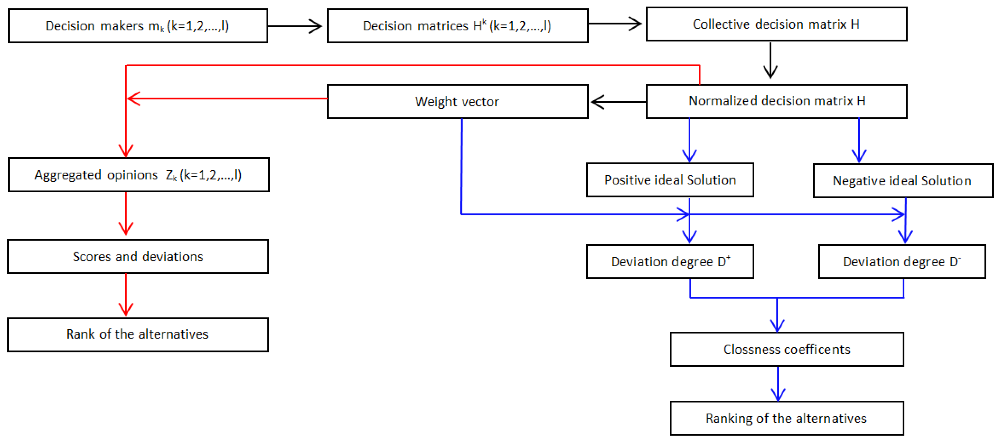
The flow chart of the proposed models is presented in Figure 1.

6. A Case Study

To validate the proposed theory and decision making models, in this section, a practical example taken from [28] is solved. A group of seven peoples $m_l$$\left(l=1,2,3,\dots ,7\right)$ need to invest their savings in a most profitable way. They considered five possibilities: $x_1$ is real estate, $x_2$ is stock market, $x_3$ is T-bills, $x_4$ is national saving scheme, and $x_5$ is insurance company. To determine best option, the following attributes are taken into account: $c_1$ is the risk factor, $c_2$ is the growth, $c_3$ is quick refund, and $c_4$ is complicated documents requirement. Base upon their knowledge and experience, they provide their opinion in terms of following HIFLTSs.

6.1. The Extended TOPSIS Method for the Considered Case

We handle the above problem by applying the extended TOPSIS method.

Step 1: The probabilistic hesitant intuitionistic linguistic decision matrices derived from

Table 1. Decision matrix provided by the DMs 1, 2, 3 $(m_1,m_2,m_3)$.

	c${}_1$	c${}_2$	c${}_3$	c${}_4$
x${}_1$	$〈\left\{s_3,s_4,s_5\right\},\left\{s_1,s_2\right\}〉$	$〈\left\{s_4,s_5\right\},\left\{s_0,s_1\right\}〉$	$〈\left\{s_1,s_2\right\},\left\{s_3,s_4\right\}〉$	$〈\left\{s_1,s_2\right\},\left\{s_3,s_4\right\}〉$
x${}_2$	$〈\left\{s_1,s_2\right\},\left\{s_3,s_4\right\}〉$	$〈\left\{s_3,s_4,s_5\right\},\left\{s_1,s_2\right\}〉$	$〈\left\{s_3,s_4\right\},\left\{s_0,s_1\right\}〉$	$〈\left\{s_4,s_5\right\},\left\{s_1,s_2\right\}〉$
x${}_3$	$〈\left\{s_4,s_5)\right\},\left\{s_0,s_1,s_2\right\}〉$	$〈\left\{s_3,s_4\right\},\left\{s_1,s_2\right\}〉$	$〈\left\{s_5,s_6\right\},\left\{s_0\right\}〉$	$〈\left\{s_1,s_2\right\},\left\{s_2,s_3,s_4\right\}〉$
x${}_4$	$〈\left\{s_5,s_6\right\},\left\{s_0,s_1\right\}〉$	$〈\left\{s_1,s_2\right\},\left\{s_3,s_4\right\}〉$	$〈\left\{s_1,s_2\right\},\left\{s_3,s_4\right\}〉$	$〈\left\{s_3,s_4,s_5\right\},\left\{s_1,s_2\right\}〉$
x${}_5$	$〈\left\{s_6\right\},\left\{s_0\right\}〉$	$〈\left\{s_1,s_2\right\},\left\{s_3,s_4,s_5\right\}〉$	$〈\left\{s_0,s_1\right\},\left\{s_2,s_3\right\}〉$	$〈\left\{s_4,s_5\right\},\left\{s_1,s_2\right\}〉$

,

Table 2. Decision matrix provided by the DMs 4, 5 $(m_4,m_5)$.

	c${}_1$	c${}_2$	c${}_3$	c${}_4$
x${}_1$	$〈\left\{s_1,s_2\right\},\left\{s_3,s_4\right\}〉$	$〈\left\{s_5,s_6\right\},\left\{s_0,s_1\right\}〉$	$〈\left\{s_0,s_1\right\},\left\{s_3,s_4\right\}〉$	$〈\left\{s_3,s_4\right\},\left\{s_1,s_2\right\}〉$
x${}_2$	$〈\left\{s_0,s_1\right\},\left\{s_2,s_3\right\}〉$	$〈\left\{s_1,s_2\right\},\left\{s_2,s_3,s_4\right\}〉$	$〈\left\{s_4,s_5\right\},\left\{s_0,s_1\right\}〉$	$〈\left\{s_5,s_6\right\},\left\{s_0\right\}〉$
x${}_3$	$〈\left\{s_3,s_4\right\},\left\{s_0,s_1\right\}〉$	$〈\left\{s_1,s_2\right\},\left\{s_3,s_4\right\}〉$	$〈\left\{s_4,s_5\right\},\left\{s_1,s_2)\right\}〉$	$〈\left\{s_0,s_1\right\},\left\{s_2,s_3\right\}〉$
x${}_4$	$〈\left\{s_5,s_6\right\},\left\{s_0\right\}〉$	$〈\left\{s_3,s_4\right\},\left\{s_0,s_1,s_2\right\}〉$	$〈\left\{s_1,s_2\right\},\left\{s_2,s_3,s_4\right\}〉$	$〈\left\{s_4,s_5\right\},\left\{s_0\right\}〉$
x${}_5$	$〈\left\{s_4,s_5\right\},\left\{s_1,s_2\right\}〉$	$〈\left\{s_3,s_4\right\},\left\{s_1,s_2,s_3\right\}〉$	$〈\left\{s_1,s_2\right\},\left\{s_3,s_4\right\}〉$	$〈\left\{s_5,s_6\right\},\left\{s_0\right\}〉$

and

Table 3. Decision matrix provided by the DMs 6, 7 $(m_6,m_7)$.

	c${}_1$	c${}_2$	c${}_3$	c${}_4$
x${}_1$	$〈\left\{s_4,s_5\right\},\left\{s_0,s_1\right\}〉$	$〈\left\{s_5,s_6\right\},\left\{s_0\right\}〉$	$〈\left\{s_3,s_4\right\},\left\{s_1,s_2\right\}〉$	$〈\left\{s_0,s_1\right\},\left\{s_3,s_4\right\}〉$
x${}_2$	$〈\left\{s_3,s_4\right\},\left\{s_1,s_2,s_3\right\}〉$	$〈\left\{s_1,s_2\right\},\left\{s_3,s_4\right\}〉$	$〈\left\{s_5,s_6\right\},\left\{s_0\right\}〉$	$〈\left\{s_3,s_4\right\},\left\{s_1,s_2\right\}〉$
x${}_3$	$〈\left\{s_1,s_2\right\},\left\{s_2,s_3,s_4\right\}〉$	$〈\left\{s_5,s_6\right\},\left\{s_0\right\}〉$	$〈\left\{s_4,s_5\right\},\left\{s_0,s_1\right\}〉$	$〈\left\{s_0,s_1\right\},\left\{s_3,s_4\right\}〉$
x${}_4$	$〈\left\{s_4,s_5\right\},\left\{s_1,s_2\right\}〉$	$〈\left\{s_4,s_5\right\},\left\{s_0,s_1\right\}〉$	$〈\left\{s_0,s_1,s_2\right\},\left\{s_2,s_3\right\}〉$	$〈\left\{s_3,s_4,s_5\right\},\left\{s_1,s_2\right\}〉$
x${}_5$	$〈\left\{s_3,s_4\right\},\left\{s_0,s_1,s_2\right\}〉$	$〈\left\{s_1,s_2\right\},\left\{s_2,s_3,s_4\right\}〉$	$〈\left\{s_2,s_3\right\},\left\{s_3,s_4\right\}〉$	$〈\left\{s_6\right\},\left\{s_0\right\}〉$

are shown in

Table 4. Probabilistic hesitant intuitionistic linguistic decision matrix $H_1$ with respect to DMs 1, 2, 3 $\left(m_1,m_2,m_3\right).$

	c${}_1$	c${}_2$
x${}_1$	$〈\left\{\left(s_3\left(0.14\right),s_4\left(0.28\right),s_5\left(0.28\right)\right)\right\},\left\{s_1\left(0.28\right),s_2\left(0.14\right)\right\}〉$	$〈\left\{s_4\left(0.14\right),s_5\left(0.42\right)\right\},\left\{s_0\left(0.42\right),s_1\left(0.28\right)\right\}〉$
x${}_2$	$〈\left\{s_1\left(0.28\right),s_2\left(0.14\right)\right\},\left\{s_3\left(0.42\right),s_4\left(0.14\right)\right\}〉$	$〈\left\{s_3\left(0.14\right),s_4\left(.14\right),s_5\left(0.14\right)\right\},\left\{s_1\left(0.14\right),s_2\left(0.28\right)\right\}〉$
x${}_3$	$〈\left\{s_4\left(0.28\right),s_5\left(0.14\right)\right\},\left\{s_0\left(0.28\right),s_1\left(0.28\right),s_2\left(0.28\right)\right\}〉$	$〈\left\{s_3\left(0.14\right),s_4\left(0.28\right)\right\},\left\{s_1\left(0.14\right),s_2\left(0.14\right)\right\}〉$
x${}_4$	$〈\left\{s_5\left(0.42\right),s_6\left(0.28\right)\right\},\left\{s_0\left(0.28\right),s_1\left(0.28\right)\right\}〉$	$〈\left\{s_1\left(0.14\right),s_2\left(0.14\right)\right\},\left\{s_3\left(0.14\right),s_4\left(0.14\right)\right\}〉$
x${}_5$	$〈\left\{s_6\left(0.14\right)\right\},\left\{s_0\left(0.28\right)\right\}〉$	$〈\left\{s_1\left(0.28\right),s_2\left(0.28\right)\right\},\left\{s_3\left(0.42\right),s_4\left(0.28\right),s_5\left(0.14\right)\right\}〉$
	c${}_{\mathbf{3}}$	c${}_{\mathbf{4}}$
x${}_1$	$〈\left\{s_1\left(0.28\right),s_2\left(0.14\right)\right\},\left\{s_3\left(0.28\right),s_4\left(0.28\right)\right\}〉$	$〈\left\{s_1\left(0.28\right),s_2\left(0.14\right)\right\},\left\{s_3\left(0.28\right),s_4\left(0.28\right)\right\}〉$
x${}_2$	$〈\left\{s_3\left(0.14\right),s_4\left(0.28\right)\right\},\left\{s_0\left(0.42\right),s_1\left(0.28\right)\right\}〉$	$〈\left\{s_4\left(0.14\right),s_5\left(0.28\right)\right\},\left\{s_1\left(0.28\right),s_2\left(0.28\right)\right\}〉$
x${}_3$	$〈\left\{s_5\left(0.42\right),s_6\left(0.14\right)\right\},\left\{s_0\left(0.28\right)\right\}〉$	$〈\left\{s_1\left(0.42\right),s_2\left(0.14\right)\right\},\left\{s_2\left(0.28\right),s_3\left(0.42\right),s_4\left(0.28\right)\right\}〉$
x${}_4$	$〈\left\{s_1\left(0.42\right),s_2\left(.42\right)\right\},\left\{s_3\left(0.42\right),s_4\left(0.28\right)\right\}〉$	$〈\left\{s_3\left(0.28\right),s_4\left(0.42\right),s_5\left(0.42\right)\right\},\left\{s_1\left(0.28\right),s_2\left(0.28\right)\right\}〉$
x${}_5$	$〈\left\{s_0\left(0.14\right),s_1\left(0.28\right)\right\},\left\{s_2\left(0.28\right),s_3\left(0.42\right)\right\}〉$	$〈\left\{s_4\left(0.14\right),s_5\left(0.28\right)\right\},\left\{s_1\left(0.14\right),s_2\left(0.14\right)\right\}〉$

,

Table 5. Probabilistic hesitant intuitionistic linguistic decision matrix $H_2$ with respect to DMs $4,5\left(m_4,m_5\right)$.

	c${}_1$	c${}_2$
x${}_1$	$〈\left\{s_1\left(0.14\right),s_2\left(0.14\right)\right\},\left\{s_3\left(0.14\right),s_4\left(0.14\right)\right\}〉$	$〈\left\{s_5\left(0.42\right),s_6\left(0.28\right)\right\},\left\{s_0\left(0.42\right),s_1\left(0.28\right)\right\}〉$
x${}_2$	$〈\left\{s_0\left(0.14\right),s_1\left(0.28\right)\right\},\left\{s_2\left(0.28\right),s_3\left(0.42\right)\right\}〉$	$〈\left\{s_1\left(0.28\right),s_2\left(0.28\right)\right\},\left\{s_2\left(0.28\right),s_3\left(0.28\right),s_4\left(0.28\right)\right\}〉$
x${}_3$	$〈\left\{s_3\left(0.14\right),s_4\left(.28\right)\right\},\left\{s_0\left(0.28\right),s_1\left(0.28\right)\right\}〉$	$〈\left\{s_1\left(0.14\right),s_2\left(0.14\right)\right\},\left\{s_3\left(0.14\right),s_4\left(0.14\right)\right\}〉$
x${}_4$	$〈\left\{s_5\left(0.42\right),s_6\left(0.28\right)\right\},\left\{s_0\left(0.28\right)\right\}〉$	$〈\left\{s_3\left(0.14\right),s_4\left(0.28\right)\right\},\left\{s_0\left(0.28\right),s_1\left(0.28\right),s_2\left(0.14\right)\right\}〉$
x${}_5$	$〈\left\{s_4\left(0.28\right),s_5\left(0.14\right)\right\},\left\{s_1\left(0.28\right),s_2\left(0.28\right)\right\}〉$	$〈\left\{s_3\left(0.14\right),s_4\left(0.14\right)\right\},\left\{s_1\left(0.14\right),s_2\left(0.28\right),s_3\left(0.42\right)\right\}〉$
	c${}_{\mathbf{3}}$	c${}_{\mathbf{4}}$
x${}_1$	$〈\left\{s_{0.}\left(0.14\right),s_1\left(0.28\right)\right\},\left\{s_3\left(0.28\right),s_4\left(0.28\right)\right\}〉$	$〈\left\{s_3\left(0.14\right),s_4\left(0.14\right)\right\},\left\{s_1\left(0.14\right),s_2\left(0.14\right)\right\}〉$
x${}_2$	$〈\left\{s_4\left(0.28\right),s_5\left(0.28\right)\right\},\left\{s_0\left(0.42\right),s_1\left(0.28\right)\right\}〉$	$〈\left\{s_5\left(0.28\right),s_6\left(0.14\right)\right\},\left\{s_0\left(0.14\right)\right\}〉$
x${}_3$	$〈\left\{s_4\left(0.28\right),s_5\left(0.42\right)\right\},\left\{s_1\left(0.28\right),s_2\left(0.14\right)\right\}〉$	$〈\left\{s_0\left(0.28\right),s_1\left(0.42\right)\right\},\left\{s_2\left(0.28\right),s_3\left(0.42\right)\right\}〉$
x${}_4$	$〈\left\{s_1\left(0.42\right),s_2\left(0.42\right)\right\},\left\{s_2\left(0.28\right),s_3\left(0.42\right),s_4\left(0.28\right)\right\}〉$	$〈\left\{s_4\left(0.42\right),s_5\left(0.42\right)\right\},\left\{s_0\left(0.14\right)\right\}〉$
x${}_5$	$〈\left\{s_1\left(0.28\right),s_2\left(0.14\right)\right\},\left\{s_3\left(0.42\right),s_4\left(0.28\right)\right\}〉$	$〈\left\{s_5\left(0.28\right),s_6\left(0.28\right)\right\},\left\{s_0\left(0.28\right)\right\}〉$

and

Table 6. Probabilistic hesitant intuitionistic linguistic decision matrix $H_3$ with respect to DMs $6,7\left(m_6,m_7\right)$.

	c${}_1$	c${}_2$
x${}_1$	$〈\left\{s_4\left(0.28\right),s_5\left(0.28\right)\right\},\left\{s_0\left(0.14\right),s_1\left(0.28\right)\right\}〉$	$〈\left\{s_5\left(0.42\right),s_6\left(0.28\right)\right\},\left\{s_0\left(0.42\right)\right\}〉$
x${}_2$	$〈\left\{s_3\left(0.14\right),s_4\left(0.14\right)\right\},\left\{s_1\left(0.14\right),s_2\left(0.28\right),s_3\left(0.42\right)\right\}〉$	$〈\left\{s_1\left(0.28\right),s_2\left(0.28\right)\right\},\left\{s_3\left(0.28\right),s_4\left(0.28\right)\right\}〉$
x${}_3$	$〈\left\{s_1\left(0.14\right),s_2\left(0.14\right)\right\},\left\{s_2\left(0.28\right),s_3\left(0.14\right),s_4\left(0.14\right)\right\}〉$	$〈\left\{s_5\left(0.28\right),s_6\left(0.14\right)\right\},\left\{s_0\left(0.14\right)\right\}〉$
x${}_4$	$〈\left\{s_4\left(0.14\right),s_5\left(0.42\right)\right\},\left\{s_1\left(0.28\right),s_2\left(0.14\right)\right\}〉$	$〈\left\{s_4\left(0.28\right),s_5\left(0.14\right)\right\},\left\{s_0\left(0.28\right),s_1\left(0.28\right)\right\}〉$
x${}_5$	$〈\left\{s_3\left(0.14\right),s_4\left(0.28\right)\right\},\left\{s_0\left(0.28\right),s_1\left(0.28\right),s_2\left(0.28\right)\right\}〉$	$〈\left\{s_1\left(0.28\right),s_2\left(0.28\right)\right\},\left\{s_2\left(0.28\right),s_3\left(0.42\right),s_4\left(0.28\right)\right\}〉$
	c${}_{\mathbf{3}}$	c${}_{\mathbf{4}}$
x${}_1$	$〈\left\{s_3\left(0.14\right),s_4\left(0.14\right)\right\},\left\{s_1\left(0.14\right),s_2\left(0.14\right)\right\}〉$	$〈\left\{s_0\left(0.14\right),s_1\left(0.28\right)\right\},\left\{s_3\left(0.28\right),s_4\left(0.28\right)\right\}〉$
x${}_2$	$〈\left\{s_5\left(0.28\right),s_6\left(0.14\right)\right\},\left\{s_0\left(.42\right)\right\}〉$	$〈\left\{s_3\left(0.14\right),s_4\left(0.28\right)\right\},\left\{s_1\left(0.28\right),s_2\left(0.28\right)\right\}〉$
x${}_3$	$〈\left\{s_4\left(0.28\right),s_5\left(0.42\right)\right\},\left\{s_0\left(0.28\right),s_1\left(0.28\right)\right\}〉$	$〈\left\{s_0\left(0.28\right),s_1\left(0.42\right)\right\},\left\{s_3\left(0.42\right),s_4\left(0.28\right)\right\}〉$
x${}_4$	$〈\left\{s_0\left(0.14\right),s_1\left(0.42\right),s_2\left(0.42\right)\right\},\left\{s_2\left(0.28\right),s_3\left(0.42\right)\right\}〉$	$〈\left\{s_3\left(0.28\right),s_4\left(0.42\right),s_5\left(0.42\right)\right\},\left\{s_1\left(0.28\right),s_2\left(0.28\right)\right\}〉$
x${}_5$	$〈\left\{s_2\left(0.14\right),s_3\left(0.14\right)\right\},\left\{s_3\left(0.28\right),s_4\left(0.28\right)\right\}〉$	$〈\left\{s_6\left(0.28\right)\right\},\left\{s_0\left(0.28\right)\right\}〉$

, respectively.

Step 2: The decision matrix H in

Table 7. Decision matrix (H).

	c${}_1$	c${}_2$
x${}_1$	$〈\left\{s_2\left(0.14\right),s_4\left(0.28\right)\right\},\left\{s_1\left(0.28\right),s_3\left(0.14\right)\right\}〉$	$〈\left\{s_6\left(0.28\right),s_5\left(0.42\right)\right\},\left\{s_0\left(0.42\right),s_0\left(0.42\right)\right\}〉$
x${}_2$	$〈\left\{s_1\left(0.28\right),s_3\left(0.14\right)\right\},\left\{s_4\left(0.14\right),s_3\left(0.42\right)\right\}〉$	$〈\left\{s_2\left(0.28\right),s_3\left(0.14\right)\right\},\left\{s_2\left(0.28\right),s_3\left(0.28\right)\right\}〉$
x${}_3$	$〈\left\{s_2\left(0.14\right),s_0\left(0.14\right)\right\},\left\{s_1\left(0.28\right),s_3\left(0.14\right)\right\}〉$	$〈\left\{s_2\left(0.14\right),s_6\left(0.14\right)\right\},\left\{s_0\left(0.14\right),s_3\left(0.14\right)\right\}〉$
x${}_4$	$〈\left\{s_6\left(0.28\right),s_5\left(0.42\right)\right\},\left\{s_0\left(0.28\right),s_1\left(0.28\right)\right\}〉$	$〈\left\{s_2\left(0.14\right),s_5\left(0.14\right)\right\},\left\{s_1\left(0.28\right),s_3\left(0.14\right)\right\}〉$
x${}_5$	$〈\left\{s_6\left(0.14\right),s_6\left(0.14\right)\right\},\left\{s_0\left(0.28\right),s_1\left(0.28\right)\right\}〉$	$〈\left\{s_3\left(0.14\right),s_2\left(0.28\right)\right\},\left\{s_5\left(0.14\right),s_3\left(0.42\right)\right\}〉$
	c${}_{\mathbf{3}}$	c${}_{\mathbf{4}}$
x${}_1$	$〈\left\{s_1\left(0.28\right),s_3\left(0.14\right)\right\},\left\{s_2\left(0.14\right),s_3\left(0.28\right)\right\}〉$	$〈\left\{s_1\left(0.28\right),s_3\left(0.14\right)\right\},\left\{s_2\left(0.14\right),s_3\left(0.28\right)\right\}〉$
x${}_2$	$〈\left\{s_4\left(0.28\right),s_4\left(0.14\right)\right\},\left\{s_0\left(0.42\right),s_0\left(0.42\right)\right\}〉$	$〈\left\{s_1\left(0.28\right),s_3\left(0.14\right)\right\},\left\{s_0\left(0.14\right),s_3\left(0.28\right)\right\}〉$
x${}_3$	$〈\left\{s_4\left(0.28\right),s_5\left(0.42\right)\right\},\left\{s_0\left(0.28\right),s_1\left(0.28\right)\right\}〉$	$〈\left\{s_1\left(0.14\right),s_2\left(0.42\right)\right\},\left\{s_4\left(0.28\right),s_3\left(0.42\right)\right\}〉$
x${}_4$	$〈\left\{s_1\left(0.42\right),s_2\left(0.42\right)\right\},\left\{s_{4.}\left(0.28\right),s_3\left(0.42\right)\right\}〉$	$〈\left\{s_4\left(0.42\right),s_5\left(0.42\right)\right\},\left\{s_0\left(0.14\right),s_2\left(0.28\right)\right\}〉$
x${}_5$	$〈\left\{s_1\left(0.28\right),s_2\left(0.14\right)\right\},\left\{s_{4.}\left(0.28\right),s_3\left(0.42\right)\right\}〉$	$〈\left\{s_5\left(0.28\right),s_6\left(0.28\right)\right\},\left\{s_0\left(0.28\right),s_1\left(0.14\right)\right\}〉$

is constructed by utilizing Table 4, Table 5 and Table 6.

Step 3: The normalized probabilistic hesitant intuitionistic linguistic decision matrix of the group is shown in

Table 8. The normalized probabilistic hesitant intuitionistic linguistic decision matrix.

	c${}_1$
x${}_1$	$〈\left\{s_4\left(0.6666667\right),s_2\left(0.3333333\right)\right\},\left\{s_3\left(0.3333333\right),s_1\left(0.6666667\right)\right\}〉$
x${}_2$	$〈\left\{s_3\left(0.3333333\right),s_1\left(0.6666667\right)\right\},\left\{s_3\left(0.75\right),s_4\left(0.25\right)\right\}〉$
x${}_3$	$〈\left\{s_0\left(0.5\right),s_2\left(0.5\right)\right\},\left\{s_3\left(0.3333333\right),s_1\left(0.6666667\right)\right\}〉$
x${}_4$	$〈\left\{s_5\left(0.6\right),s_6\left(0.4\right)\right\},\left\{s_1\left(0.5\right),s_0\left(0.5\right)\right\}〉$
x${}_5$	$〈\left\{s_6\left(0.5\right),s_6\left(0.5\right)\right\},\left\{s_0\left(0.5\right),s_1\left(0.5\right)\right\}〉$
	c${}_{\mathbf{2}}$
x${}_1$	$〈\left\{s_5\left(0.6\right),s_6\left(0.4\right)\right\},\left\{s_0\left(0.5\right),s_0\left(0.5\right)\right\}〉$
x${}_2$	$〈\left\{s_3\left(0.3333333\right),s_2\left(0.6666667\right)\right\},\left\{s_3\left(0.5\right),s_2\left(0.5\right)\right\}〉$
x${}_3$	$〈\left\{s_6\left(0.5\right),s_2\left(0.5\right)\right\},\left\{s_3\left(0.5\right),s_0\left(0.5\right)\right\}〉$
x${}_4$	$〈\left\{s_5\left(0.5\right),s_2\left(0.5\right)\right\},\left\{s_3\left(0.3333333\right),s_1\left(0.6666667\right)\right\}〉$
x${}_5$	$〈\left\{s_2\left(0.6666667\right),s_3\left(0.3333333\right)\right\},\left\{s_3\left(0.75\right),s_5\left(0.25\right)\right\}〉$
	c${}_{\mathbf{3}}$
x${}_1$	$〈\left\{s_3\left(0.3333333\right),s_1\left(0.6666667\right)\right\},\left\{s_3\left(0.6666667\right),s_2\left(0.3333333\right)\right\}〉$
x${}_2$	$〈\left\{s_4\left(0.6666667\right),s_4\left(0.3333333\right)\right\},\left\{s_0\left(0.5\right),s_0\left(0.5\right)\right\}〉$
x${}_3$	$〈\left\{s_5\left(0.6\right),s_4\left(0.4\right)\right\},\left\{s_5\left(0.6\right),s_4\left(0.4\right)\right\}〉$
x${}_4$	$〈\left\{s_1\left(0.5\right),s_2\left(0.5\right)\right\},\left\{s_3\left(0.6\right),s_{4.}\left(0.4\right)\right\}〉$
x${}_5$	$〈\left\{s_1\left(0.6666667\right),s_2\left(0.3333333\right)\right\},\left\{s_3\left(0.6\right),s_4\left(0.4\right)\right\}〉$
	c${}_{\mathbf{4}}$
x${}_1$	$〈\left\{s_3\left(0.3333333\right),s_1\left(0.6666667\right)\right\},\left\{s_3\left(0.6666667\right),s_2\left(0.3333333\right)\right\}〉$
x${}_2$	$〈\left\{s_3\left(0.3333333\right),s_1\left(0.6666667\right)\right\},\left\{s_3\left(0.6666667\right),s_0\left(0.3333333\right)\right\}〉$
x${}_3$	$〈\left\{s_2\left(0.75\right),s_1\left(0.25\right)\right\},\left\{s_3\left(0.6\right),s_4\left(0.4\right)\right\}〉$
x${}_4$	$〈\left\{s_5\left(0.5\right),s_4\left(0.5\right)\right\},\left\{s_0\left(0.3333333\right),s_2\left(0.6666667\right)\right\}〉$
x${}_5$	$〈\left\{s_6\left(0.5\right),s_5\left(0.5\right)\right\},\left\{s_1\left(0.3333333\right),s_0\left(0.6666667\right)\right\}〉$

.

Step 4: The weight vector is derived from Equation (26) as follows:

$w={\left(0.2715,0.2219,0.2445,0.2621\right)}^t$

Step 5: The PHILTS-PIS “$A^{+}$” and the PHILTS-NIS “$A^{-}$” of each alternative are derived using Equations (27) and (28) as follows:

$A^{+}=\left(〈\left\{3,3\right\},\left\{0,0\right\}〉,〈\left\{3,2.4\right\},\left\{0,0\right\}〉,〈\left\{3,1.6\right\},\left\{0,0\right\}〉,〈\left\{3,2.5\right\},\left\{0,0\right\}〉\right)$

$A^{-}=\left(〈\left\{0,0.661\right\},\left\{2.25,1\right\}〉,〈\left\{1,1\right\},\left\{2.25,1.25\right\}〉,〈\left\{.5,0.66\right\},\left\{2,1.6\right\}〉,〈\left\{1,0.2\right\},\left\{2,1.6\right\}〉\right)$

$D\left(x_1,A^{+}\right)=2.1211,$$D\left(x_2,A^{+}\right)=2.5516,$$D\left(x_3,A^{+}\right)=2.9129,$$D\left(x_4,A^{+}\right)=1.7999,$$D\left(x_5,A^{+}\right)=1.6494$

$D\left(x_1,A^{-}\right)=2.0142,$$D\left(x_2,A^{-}\right)=1.5861,$$D\left(x_3,A^{-}\right)=1.6204,$$D\left(x_4,A^{-}\right)=2.4056,$$D\left(x_5,A^{-}\right)=2.2812$

Step 7: Calculate $D_{min}\left(x_i,A^{+}\right)$ and $D_{max}\left(x_i,A^{-}\right)$ by Equations (31) and (32) :

$D_{min}\left(x_i,A^{+}\right)=1.6494,$$D_{max}\left(x_i,A^{-}\right)=2.4050$

Step 8: Determine the closeness coefficient of each alternative $x_i$ by Equation (33) :

$Cl\left(x_1\right)=-0.4486,$$Cl\left(x_2\right)=-0.8876,$$Cl\left(x_3\right)=-1.0924,$$Cl\left(x_4\right)=-0.0912,$$Cl\left(x_5\right)=-0.0519$

Step 9: Rank the alternatives according to the ranking of $Cl\left(x_i\right)\left(i=1,2,\dots ,5\right)$: $x_5>x_4>x_1>x_2>x_3,$ and thus, $x_5$(insurance company) is the best alternative.

6.2. The Aggregation-Based Method for the Considered Case

We can also apply the aggregation-based method to attain the ranking of alternatives for the case study.

Step 1: Construct the probabilistic hesitant intuitionistic fuzzy decision matrices of the group as listed in Table 4, Table 5 and Table 6, and then aggregated and normalized as shown in Table 7 and Table 8.

Step 2: Utilize Equation (26) to obtain the weight vector

$w={\left(0.2715,0.2219,0.2445,0.2621\right)}^t.$

Step 3: Derive the overall attribute value of each alternative $x_i$ $\left(i=1,2,3,4,5\right)$ by using Equation (35) :

$\widetilde{Z_1}\left(w\right)=〈\left\{s_{1.8962},s_{0.5187}\right\},\left\{s_{1.2847},s_{0.5187}\right\}〉,$

$\widetilde{Z_2}\left(w\right)=〈\left\{s_{1.4074},s_{0.9776}\right\},\left\{s_{1.4679},s_{0.4934}\right\}〉,$

$\widetilde{Z_3}\left(w\right)=\left\{s_{1.7923},s_{1.1256}\right\},\left\{s_{1.8096},s_{0.9915}\right\},$

$\widetilde{Z_4}\left(w\right)=〈\left\{s_{2.1467},s_{1.642}\right\},\left\{s_{0.7977},s_{0.8886}\right\}〉,$

$\widetilde{Z_5}\left(w\right)=〈\left\{s_{2.0596},s_{1.8546}\right\},\left\{s_{1.0267},s_{0.8043}\right\}〉.$

Step 4: Compute the score of each attribute value $\widetilde{Z_i}\left(w\right)$ by Definition 14:

$E\left(\widetilde{Z_1}\left(w\right)\right)=s_{3.1528}$, $E\left(\widetilde{Z_2}\left(w\right)\right)=s_{3.1059}$, $E\left(\widetilde{Z_3}\left(w\right)\right)=s_{3.0584}$, $E\left(\widetilde{Z_4}\left(w\right)\right)=s_{4.0512}$, $E\left(\widetilde{Z_5}\left(w\right)\right)=s_{5.8726}$

Step 5: Compare the overall attribute values of alternatives according to the values of the score function. It is obvious, that $x_5>x_4>x_1>x_2>x_3.$ Thus, again, we get the best alternative $x_5.$

7. Discussions and Comparison

For the purpose of comparison, in this subsection, the case study is again solved by applying the TOPSIS method with traditional HIFLTSs.

Step 1: The decision matrix X in

Table 9. Decision matrix (X).

	c${}_1$	c${}_2$	c${}_3$	c${}_4$
x${}_1$	$\left(\left[s_2,s_4\right],\left[s_1,s_3\right]\right)$	$\left(\left[s_5,s_5\right],\left[s_0,s_0\right]\right)$	$\left(\left[s_1,s_3\right],\left[s_2,s_3\right]\right)$	$\left(\left[s_1,s_3\right],\left[s_2,s_3\right]\right)$
x${}_2$	$\left(\left[s_1,s_3\right],\left[s_3,s_3\right]\right)$	$\left(\left[s_2,s_3\right],\left[s_2,s_3\right]\right)$	$\left(\left[s_4,s_5\right],\left[s_0,s_0\right]\right)$	$\left(\left[s_4,s_5\right],\left[s_0,s_1\right]\right)$
x${}_3$	$\left(\left[s_2,s_4\right],\left[s_1,s_2\right]\right)$	$\left(\left[s_3,s_5\right],\left[s_0,s_3\right]\right)$	$\left(\left[s_5,s_5\right],\left[s_0,s_1\right]\right)$	$\left(\left[s_1,s_1\right],\left[s_3,s_3\right]\right)$
x${}_4$	$\left(\left[s_5,s_5\right],\left[s_0,s_1\right]\right)$	$\left(\left[s_2,s_4\right],\left[s_1,s_3\right]\right)$	$\left(\left[s_1,s_2\right],\left[s_3,s_3\right]\right)$	$\left(\left[s_4,s_5\right],\left[s_1,s_2\right]\right)$
x${}_5$	$\left(\left[s_4,s_6\right],\left[s_0,s_1\right]\right)$	$\left(\left[s_2,s_3\right],\left[s_3,s_3\right]\right)$	$\left(\left[s_1,s_2\right],\left[s_3,s_3\right]\right)$	$\left(\left[s_5,s_6\right],\left[s_0,s_1\right]\right)$

is constructed by utilizing Table 1, Table 2 and Table 3 as follows:

Step 2: Determine the HIFLTS-PIS “$P^{+}$” and the HIFLTS-NIS “$P^{-}$” for cost criteria c${}_1,$c${}_4$ and benefit criteria c${}_2$,c${}_3$ as follows:

$P^{+}=\left[\left(\left[s_0,s_1\right],\left[s_3,s_4\right]\right),\left(\left[s_5,s_6\right],\left[s_0,s_0\right]\right),\left(\left[s_5,s_6\right],\left[s_0,s_0\right]\right),\left(\left[s_0,s_1\right],\left[s_3,s_4\right]\right)\right]$

$P^{-}=\left[\left(\left[s_6,s_6\right],\left[s_0,s_0\right]\right),\left(\left[s_1,s_2\right],\left[s_3,s_5\right]\right),\left(\left[s_0,s_1\right],\left[s_3,s_4\right]\right),\left(\left[s_6,s_6\right],\left[s_0,s_0\right]\right)\right]$

Note: One can see the detail of HIFLTS-PIS “$P^{+}$” and the HIFLTS-NIS “$P^{-}$” in [28].

Step 3: Calculate the positive ideal matrix $D^{+}$ and the negative ideal matrix $D^{-}$ as follows:

$D^{+}=\left[\begin{array}{c}8+1+12+5\\ 4+11+2+14\\ 9+7+2+2\\ 15+9+14+12\\ 15+12+14+16\end{array}\right]=\left[\begin{array}{c}26\\ 31\\ 20\\ 50\\ 57\end{array}\right]$

$D_{11}^{+}=d\left(x_{11},v_1^{+}\right)+d\left(x_{12},v_2^{+}\right)+d\left(x_{13},v_3^{+}\right)+d\left(x_{14},v_4^{+}\right)$ in which $d\left(x_{11},v_1^{+}\right)=d\left(\left(\left[s_2,s_4\right],\left[s_1,s_3\right]\right),\left(\left[s_0,s_1\right],\left[s_3,s_4\right]\right)\right)=|2-0|+|4-1|+|1-3|+|3-4|=8$

Other entries can be found by similar calculation.

$D^{-}=\left[\begin{array}{c}10+15+5+13\\ 14+5+15+4\\ 9+9+15+16\\ 3+7+3+6\\ 3+4+3+2\end{array}\right]=\left[\begin{array}{c}43\\ 38\\ 49\\ 19\\ 12\end{array}\right]$

Step 4: The relative closeness$\left(RC\right)$ of each alternative to the ideal solution can be obtained as follows:

$RC\left(x_1\right)=43/\left(26+43\right)=0.6232$

$RC\left(x_2\right)=38/\left(31+38\right)=0.5507$

The $RC$ of other alternatives can be find by similar calculations.

$RC\left(x_3\right)=0.7101$, $RC\left(x_4\right)=0.2754$, $RC\left(x_5\right)=0.1739$.

Step 5: The ranking of alternatives of alternatives $x_i\left(i=1,2,\dots ,5\right)$ according to the closeness coefficient $RC\left(x_i\right)$ is:

$x_3>x_1>x_2>x_4>x_5.$

• In Table 9, the disadvantages of HIFLTS are apparent because in HIFLTS the probabilities of the linguistic terms is not considered which means that all possible linguistic terms in HIFLTS have same occurrence possibility which is unrealistic, whereas the inspection of Table 7 shows that PHILTS not only contains the linguistic terms, but also considers the probabilities of linguistic terms, and, thus, PHILTS constitutes an extension of HIFLTS.
• The inspection of

  Table 10. Comparison of Results.

  TOPSIS [28]	$x_3>x_1>x_2>x_4>x_5$
  Proposed extend TOPSIS	$x_5>x_4>x_1>x_2>x_3$
  Proposed aggregation model	$x_5>x_4>x_1>x_2>x_3$

  reveals that the extended TOPSIS method and the aggregation-based method give the same best alternative $x_5$. The TOPSIS method with the traditional HIFLTSs gives $x_3$ as the best alternative.
• This difference of best alternative in Table 10 is due to the effect of probabilities of membership and non-membership linguistic terms, which highlight the critical role of probabilities. Thus, our methods are more rational to get the ranking of alternatives and further to find the best alternative.
• Extended TOPSIS method and aggregation-based method for MAGDM with PLTS information explained in [19] are more promising and better than extended TOPSIS method and aggregation-based method for MAGDM with HFLTS information. However, a clear superiority of PHILTS is that it assigns to each element the degree of belongingness and also the degree of non-belongingness along with probability. PLTS only assigns to each element a belongingness degree along with probability. Using PLTSs, various frameworks have been developed by DMs [19,29] but they are still intolerant, since there is no mean of attributing reliability or confidence information to the degree of belongingness.

The comparisons and other aspects are summarized in

Table 11. The advantages and limitations of the proposed methods.

Advantages	Limitations
1. PHILTS generalize the existing PLTS models	1. It is essential to take membership as
since PHILTS take more information from the DMs	well as non-membership probabilistic
into account.	data.
2. PHILTS is not affected by partial vagueness.	2. Its computational index is
3. PHILTS is more in line with people’s language,	high.
leading to much more fruitful decisions.
4. The attribute weights are calculated with
objectivity (without favor).

.

8. Conclusions

Because of the blurring of human thinking, sometimes it becomes difficult for experts to accurately measure the opinions in the area of the usual fuzzy set theory, even in the HIFLTSs and PLTSs. For this purpose, in this article, a new concept called PHILTS was introduced to extend the current HIFLTS and PLTS. To facilitate the calculation of the PHILTSs, a normalization process, basic operations and aggregation operators for PHILTSs are also designed. An extended TOPSIS method and aggregation based method have been proposed to solve decision ranking problems of the group with the multiple conflict criteria in PHILTS. The proposed models are compared with existing model of TOPSIS. The PLTS and HIFLTS are special cases of PHILTS, it grants the freedom to DMs to express their opinions in more dynamic way. Furthermore, the occurrence probabilities of membership and non-membership linguistic term sets greatly affects the decision making, validating the importance of designed theory and models in this manuscript. The probability is one of the best tool to handle uncertainty of future, thus our proposed models are more suitable of decision making related to the possible future scenarios. However, its arithmetic complexity is high.

In the future, all the work which has been done thus far PLTSs and HIFLTSs can be studied for PHILTS and then applied to decision making.

References

- Atanassov, K. Intuitionistic fuzzy sets. Fuzzy Sets Syst. 1986, 20, 87–96. [Google Scholar] [CrossRef]
- Torra, V. Hesitant fuzzy sets. Int. J. Intell. Syst. 2010, 25, 529–539. [Google Scholar] [CrossRef]
- Xu, Z.; Zhou, W. Consensus building with a group of decision makers under the hesitant probabilistic fuzzy environment. Fuzzy Optim. Decis. Mak. 2017, 16, 481–503. [Google Scholar] [CrossRef]
- Bashir, Z.; Rashid, T.; Wątróbski, J.; Sałabun, W.; Malik, A. Hesitant Probabilistic Multiplicative Preference Relations in Group Decision Making. Appl. Sci. 2018, 8, 398. [Google Scholar] [CrossRef]
- Alcantud, J.C.R.; Giarlotta, A. Necessary and possible hesitant fuzzy sets: A novel model for group decision making. Inf. Fusion 2019, 46, 63–76. [Google Scholar] [CrossRef]
- Zadeh, L.A. The concept of a linguistic variable and its applications to approximate reasoning. Inf. Sci. Part I II III 1975, 8–9, 43–80, 199–249, 301–357. [Google Scholar]
- Ju, Y.B.; Yang, S.H. Approaches for multi-attribute group decision making based on intuitionistic trapezoid fuzzy linguistic power aggregation operators. J. Intell. Fuzzy Syst. 2014, 27, 987–1000. [Google Scholar]
- Merigó, J.M.; Casanovas, M.; Martínez, L. Linguistic aggregation operators for linguistic decision making based on the Dempster–Shafer theory of evidence. Int. J. Uncertain. Fuzziness Knowl. Based Syst. 2010, 18, 287–304. [Google Scholar]
- Zhu, H.; Zhao, J.B.; Xu, Y. 2-Dimension linguistic computational model with 2-tuples for multi-attribute group decision making. Knowl. Based Syst. 2016, 103, 132–142. [Google Scholar] [CrossRef]
- Meng, F.Y.; Tang, J. Extended 2-tuple linguistic hybrid aggregation operators and their application to multi-attribute group decision making. Int. J. Comput. Intell. Syst. 2014, 7, 771–784. [Google Scholar] [CrossRef]
- Li, C.C.; Dong, Y. Multi-attribute group decision making methods with proportional 2-tuple linguistic assessments and weights. Int. J. Comput. Intell. Syst. 2014, 7, 758–770. [Google Scholar] [CrossRef] [Green Version]
- Xu, Z.S. Multi-period multi-attribute group decision-making under linguistic assessments. Int. J. Gen. Syst. 2009, 38, 823–850. [Google Scholar] [CrossRef]
- Li, D.F. Multiattribute group decision making method using extended linguistic variables. Int. J. Uncertain. Fuzziness Knowl. Based Syst. 2009, 17, 793–806. [Google Scholar] [CrossRef]
- Agell, N.; Sánchez, M.; Prats, F.; Roselló, L. Ranking multi-attribute alternatives on the basis of linguistic labels in group decisions. Inf. Sci. 2012, 209, 49–60. [Google Scholar] [CrossRef]
- Rodríguez, R.M.; Martínez, L.; Herrera, F. Hesitant fuzzy linguistic term sets for decision making. IEEE Trans. Fuzzy Syst. 2012, 20, 109–119. [Google Scholar]
- Zhu, J.; Li, Y. Hesitant Fuzzy Linguistic Aggregation Operators Based on the Hamacher t-norm and t-conorm. Symmetry 2018, 10, 189. [Google Scholar] [CrossRef]
- Cui, W.; Ye, J. Multiple-Attribute Decision-Making Method Using Similarity Measures of Hesitant Linguistic Neutrosophic Numbers Regarding Least Common Multiple Cardinality. Symmetry 2018, 10, 330. [Google Scholar] [CrossRef]
- Liu, D.; Liu, Y.; Chen, X. The New Similarity Measure and Distance Measure of a Hesitant Fuzzy Linguistic Term Set Based on a Linguistic Scale Function. Symmetry 2018, 10, 367. [Google Scholar] [CrossRef]
- Pang, Q.; Wang, H.; Xu, Z. Probabilistic linguistic term sets in multi-attribute group decision making. Inf. Sci. 2016, 369, 128–143. [Google Scholar] [CrossRef]
- Lin, M.; Xu, Z.; Zhai, Y.; Zhai, T. Multi-attribute group decision-making under probabilistic uncertain linguistic environment. J. Oper. Res. Soc. 2017. [Google Scholar] [CrossRef]
- Atanassov, K. Intuitionistic Fuzzy Sets; Springer: Heidelberg, Germany, 1999. [Google Scholar]
- Bashir, Z.; Rashid, T.; Wątróbski, J.; Sałabun, W.; Ali, J. Intuitionistic-fuzzy goals in zero-sum multi criteria matrix games. Symmetry 2017, 9, 158. [Google Scholar] [CrossRef]
- Beg, I.; Rashid, T. Group Decision making Using Intuitionistic Hesitant Fuzzy Sets. Int. J. Fuzzy Logic Intell. Syst. 2014, 14, 181–187. [Google Scholar] [CrossRef]
- Boran, F.E.; Gen, S.; Kurt, M.; Akay, D. A multi-criteria intuitionistic fuzzy group decision making for supplier selection with TOPSIS method. Expert Syst. Appl. 2009, 36, 11363–11368. [Google Scholar] [CrossRef]
- De, S.K.; Biswas, R.; Roy, A.R. An application of intuitionistic fuzzy sets in medical diagnosis. Fuzzy Sets Syst. 2001, 117, 209–213. [Google Scholar] [CrossRef]
- Li, D.F. Multiattribute decision making models and methods using intuitionistic fuzzy sets. J. Comput. Syst. Sci. 2005, 70, 73–85. [Google Scholar] [CrossRef]
- Liu, P.; Mahmood, T.; Khan, Q. Multi-Attribute Decision-Making Based on Prioritized Aggregation Operator under Hesitant Intuitionistic Fuzzy Linguistic Environment. Symmetry 2017, 9, 270. [Google Scholar] [CrossRef]
- Beg, I.; Rashid, T. Hesitant intuitionistic fuzzy linguistic term sets. Notes Intuit. Fuzzy Sets 2014, 20, 53–64. [Google Scholar]
- Zhang, Y.; Xu, Z.; Wang, H.; Liao, H. Consistency-based risk assessment with probablistic linguistic prefrence relation. Appl. Soft Comput. 2016, 49, 817–833. [Google Scholar] [CrossRef]
- Xu, Z.S.; Xia, M.M. On distance and correlation measures of hesitant fuzzy information. Int. J. Intell. Syst. 2011, 26, 410–425. [Google Scholar] [CrossRef]
- Kim, S.H.; Ahn, B.S. Interactive group decision making procedure under incomplete information. Eur. J. Oper. Res. 1999, 116, 498–507. [Google Scholar] [CrossRef]
- Kim, S.H.; Choi, S.H.; Kim, J.K. An interactive procedure for multiple attribute group decision making with incomplete information: Range-based approach. Eur. J. Oper. Res. 1999, 118, 139–152. [Google Scholar] [CrossRef]
- Park, K.S. Mathematical programming models for characterizing dominance and potential optimality when multicriteria alternative values and weights are simultaneously incomplete. IEEE Trans. Syst. Man Cybern. 2004, 34, 601–614. [Google Scholar] [CrossRef]
- Xu, Z.S. An interactive procedure for linguistic multiple attribute decision making with incomplete weight information. Fuzzy Optim. Decis. Mak. 2007, 6, 17–27. [Google Scholar] [CrossRef]
Figure 1.
Extended TOPSIS and Aggregation-based models.