The Application of a Double CUSUM Algorithm in Industrial Data Stream Anomaly Detection


1
School of Electrical Engineering, Zhengzhou University, Zhengzhou 450001, China
2
The 22th Research Institute of China Electronics Technology Group Corporation, Xinxiang 453003, China
*
Authors to whom correspondence should be addressed.
Symmetry 2018, 10(7), 264; https://doi.org/10.3390/sym10070264
Submission received: 8 June 2018
/
Revised: 19 June 2018
/
Accepted: 2 July 2018
/
Published: 5 July 2018
(This article belongs to the Special Issue Information Technology and Its Applications 2021)
Abstract
:The effect of the application of machine learning on data streams is influenced by concept drift, drift deviation, and noise interference. This paper proposes a data stream anomaly detection algorithm combined with control chart and sliding window methods. This algorithm is named DCUSUM-DS (Double CUSUM Based on Data Stream), because it uses a dual mean value cumulative sum. The DCUSUM-DS algorithm based on nested sliding windows is proposed to satisfy the concept drift problem; it calculates the average value of the data within the window twice, extracts new features, and then calculates accumulated and controlled graphs to avoid misleading by interference points. The new algorithm is simulated using drilling engineering industrial data. Compared with automatic outlier detection for data streams (A-ODDS) and with sliding nest window chart anomaly detection based on data streams (SNWCAD-DS), the DCUSUM-DS can account for concept drift and shield a small amount of interference deviating from the overall data. Although the algorithm complexity increased from 0.1 second to 0.19 second, the classification accuracy receiver operating characteristic (ROC) increased from 0.89 to 0.95. This meets the needs of the oil drilling industry data stream with a sampling frequency of 1 Hz, and it improves the classification accuracy.
1. Introduction
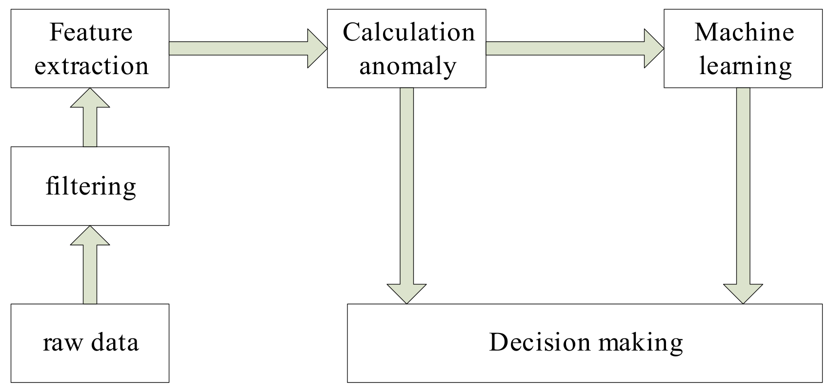
In industry and life, many application systems monitor real-time data. When an abnormal change in data is detected, several abnormal data are combined to make decisions. Such systems include oil drilling early warning systems [1], industrial sensor systems [2], internet data stream [3], medical surveillance systems [4], gas turbine fuel systems [5], the Internet of Things [6], and wind turbines [7]. A general decision system flowchart is shown in Figure 1, as follows:
As shown in Figure 1, machine learning can obtain the decision model by mining the rule of abnormal change of the parameters. When the combined parameters with the same abnormal changes are obtained, the decision model is achieved. We can see that many decision-making systems must know which parameters are abnormal before making decisions, must know the degree of abnormality, and must make corresponding decisions based on these abnormal parameters and the degree of their abnormalities.
The common features of these systems are listed as follows:
- The amount of data is practically infinite, pouring in as time goes on.
- Each piece of data has its own time stamp.
- There is concept drift, and there is no regular data distribution.
- Affected by various conditions, such as the sensor’s operating environment and its installation location, some data are distorted or ineffective and are of low quality.
Real-time decision-making requires the real-time monitoring of operating status; decisions can thus be made in real time. Based on the above, the anomaly detection algorithm applied to data streams requires a high detection accuracy and low complexity, and only one scan and one detection are allowed. The first two features are opposites (regarding accuracy and complexity), as algorithms with high detection accuracy are often more complex. For example, traditional machine learning algorithms aim toward static data classification, but their long calculation time cannot be applied to the data stream at all and therefore cannot satisfy the real-time system. Due to real-time requirements, algorithms with low complexity generally hardly achieve data stream anomaly detection accuracy. Data stream anomaly detection, including conceptual drift detection [8] and conceptual drift anomaly detection [9], can be regarded as a further analysis operation of multi-class machine learning. Based on papers published in international top conferences and international authoritative journals in the field of machine learning, data stream anomaly detection [10] research has increasingly been given academic attention for the past few years. Data streams, which exists extensively in work and life, have provided a wide range of application fields. Due to the characteristics of the data stream analyzed above, data stream machine learning has brought about great challenges. Therefore, data stream anomaly detection has transformed from single methods to cross-integration methods, such as the sliding window model [11,12], control charts [13], evolutionary calculation [14], transfer learning [15], and clustering [16]. Traditional analysis methods, such as feature selection [17], ensemble learning [18], and various pattern classification theories [19], have been transformed into data stream anomaly detection methods through combinations with sliding windows. Sliding windows and ensemble learning have been combined with data stream anomaly classification [20]; sliding windows and evolutionary algorithms have been combined with data stream anomaly detection classification [21]; and singular spectrum analysis and control charts have been combined with a real-time cardiac anomaly detection algorithm [22]. The combination of these algorithms will inevitably lead to an increase in the algorithm complexity, but with the advancement of computer technology, greater computing capability can already support the application of data stream anomaly detection algorithms in reality. The contributions of this article are the following: (1) we use nested sliding windows to enhance the trend analysis of the current point and historical data, (2) we reduce the impact weight of the current point by calculating the mean difference twice, (3) we integrate the above two points using the cumulative sum (CUSUM) algorithm, and (4) we increase the outbound rate parameter and perform real-time data stream detection.
The data stream is affected by concept drift [23]. The concept drift of machine learning represents the phenomenon that the statistical characteristics of the target variable change in an unpredictable manner over time. The data trend in the data stream changes in real time, and the current point data change is the starting point of the real concept drift or the interference point, which is a problem that the data stream machine learning algorithm needs to solve.
As shown in Figure 2, several data deviate from the normal trend at the back end, but no trend deviates continuously and quickly returns to the overall trend. Therefore, these data are disturbance data and should not be considered as abnormal data that enter into the decision model, as it will otherwise lead to late mistaken decisions. The front-end data continuously deviate from the overall trend, so it is regarded as abnormal data. Abnormal point detection and abnormality detection are required, and several abnormal parameters need to be used in the later stage to make decisions. The former abnormal data drop is the real one caused by real internal causes, which is our focus and target of detection, because the change is caused by the internal environment, the abnormal changes of these data are consistent with the goals of our decision-making. It is necessary to correctly classify this data and detect the degree of abnormality. Therefore, reducing the misclassification caused by the interference data, increasing the trend judgment, and improving the accuracy of forecasting are research directions in the field of data stream machine learning.
The difficulty of data stream anomaly detection lies in concept drift. The future distribution of a data stream is unknown. It is difficult to classify only the current data or several neighboring data. If the current data undergo a conceptual drift, subsequent data will continue and can then be regarded as true abnormal data. This type of concept drift may be caused by some kind of intrinsic mechanism. It is data that need special attention and continuous analysis. However, it is normal to return to general trends in the short term. Designing an algorithm that detects when concept drift of a data stream occurs and correctly classifies and shields interference data is difficult, and it is difficult to calculate statistics of data stream distribution. To solve such problems, the clustered data stream classification method [23] and the data stream decomposition method [24] have been proposed. Although the above methods can detect data stream anomalies while satisfying the concept drift of the data stream, there is no analysis of interference data or the real concept drift data. This paper proposes a dual mean value cumulative sum DCUSUM data stream anomaly detection method based on sliding nest window chart anomaly detection based on data streams (SNWCAD-DS). Anomaly detection is achieved using the method of control charts. This method not only can detect the concept drift of the data stream, but also can shield the influence of the interference point. Compared with the traditional data stream machine, this method improves classification accuracy, which can meet the practical needs of field engineering.
This paper first introduces the related work, then introduces the control chart algorithm of two mean calculations, simulates and compares the performance of algorithm, and finally summarizes the contribution of the paper.
2. Related Work
2.1. Sliding Window
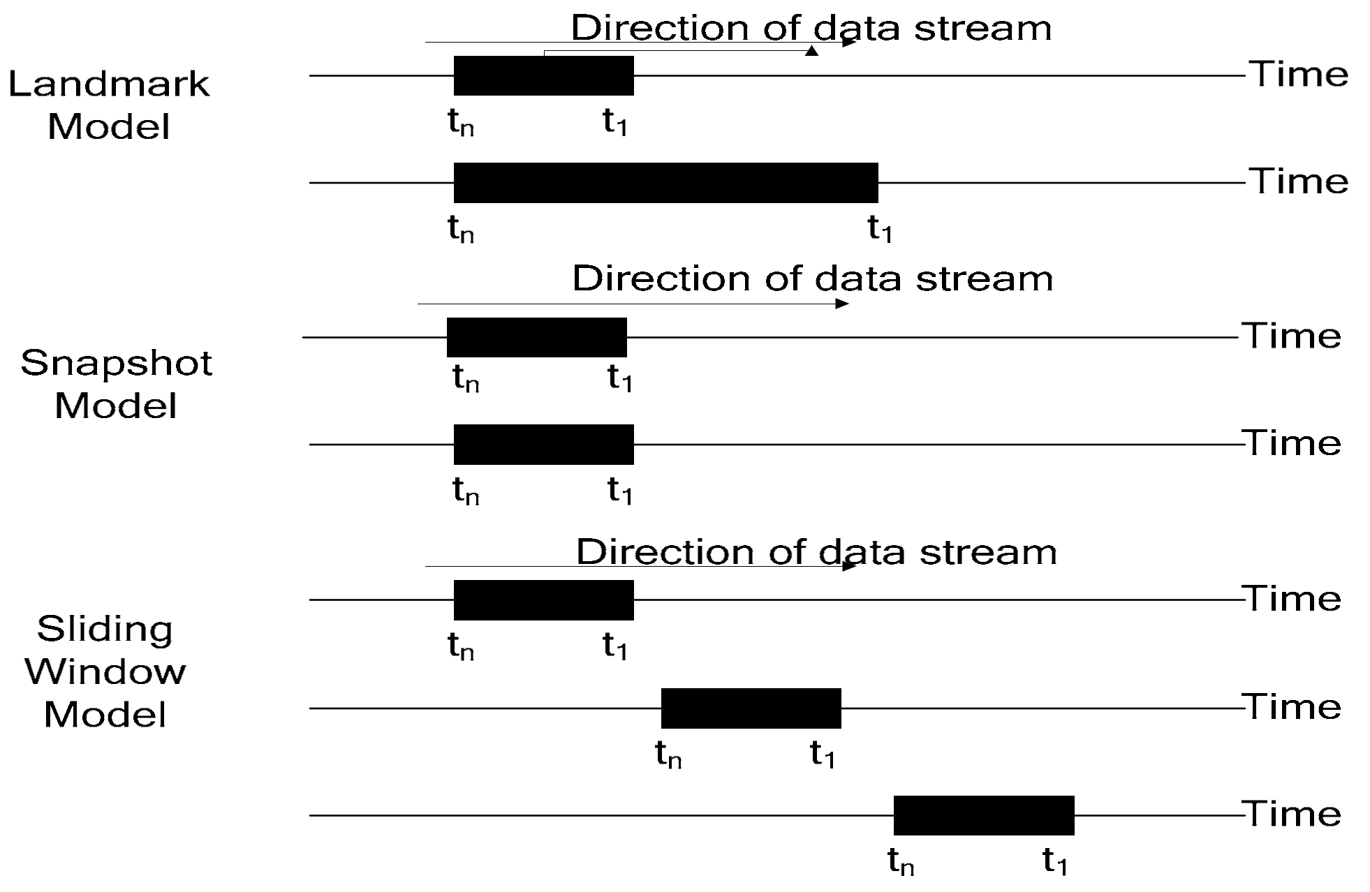
There are three kinds of window methods for the data stream: landmark [25], snapshot [26], and sliding window [2]. Due to its different working principle, the sliding window method is the most widely used.
As shown in Figure 3, the amount of data processed by the landmark model continues to increase gradually, so the algorithm only needs to respond to newly inserted data in a timely manner. The sliding window model has the same processing data range, which is always the current time data and similar fixed-length data. Therefore, when analyzing the sliding window data stream, new data should be continuously monitored, and old data should be deleted. In practical applications, the data in the most recent window from the current moment is often of great significance and research value and is usually the focus of the user’s attention. Therefore, sliding window data stream analysis method is the most widely studied and most practical method.
2.2. Theoretical Background: CUSUM
Accumulation and control map [27] calculates the difference between the current value and the mean value and accumulates these differences. The purpose is to detect the data change under the minimum delay. Based on the above analysis, we must determine the distribution of the analysis data. If there is a data stream sequence x before and after the distribution changes, then and are known. The CUSUM calculation process is as follows:
As shown in Figure 4, before the abnormal point, is always negative, so it is a linear downward trend; however, after the abnormal point appears, becomes positive and begins to show an upward trend.
As shown in Figure 4, CUSUM has a good anomaly detection effect for two simple and known distributions and can be sensitively detected for faint changes.
However, the future data distribution is unknown. Due to the randomness of the data stream, its distribution is also more complicated. Therefore, the CUSUM formula is changed to the following form:
where is the mean value, is the standard deviation, is a tunable parameter of the algorithm, and operator = max (0; S). From the above formula, we can see that the modified formula no longer uses the average value of all data as a reference value, but instead changes the mean value to a certain threshold. This has the advantage of reflecting the current data change more sensitively. The algorithm steps are shown in Algorithm 1 as follows:
| Algorithm 1 CUSUM |
| 1. CUSUM: =0, i={1,2, ,m}, 2. if , 3. and , if 4. Design parameters: bias and threshold 5. Output: alarm time(s) |
This algorithm can detect abnormal rise. The above algorithm shows that is the sum between the parameter and the reference value difference. It will be forced to 0 when the cumulative is always negative. When keeps rising and exceeds the set threshold , it will alarm and accumulate zero. We can see from the algorithm that the setting of threshold and reference value difference is very important. If and are overly small, more false positives and more false negatives will result.
3. DCUSUM-DS Algorithm
When the data stream is affected by the environment and accompanied by interference and noise, the machine learning classification is even worse. The traditional classification method has a certain time delay. In summary, the characteristics of the data stream determine that data stream machine learning cannot be classified by a single method. Combining multiple methods to classify data streams must also take into account the constraints of the algorithm complexity [28,29], which can meet the requirement of real-time online operation.
As shown in Figure 5, it is difficult to classify real time because of concept drift. Therefore, the sliding window strategy is adopted. Secondly, the window of nesting is used to reduce the sensitivity of the current data.
Two mean deviation methods are used to extract the feature quantity, and the misclassification problem caused by a few points deviating from the normal trend is masked. Finally, DCUSUM-DS are adopted. The DCUSUM-DS algorithm is summarized in Algorithm 2 as follows:
| Algorithm 2 DCUSUM-DS |
| 1. DCUSUM-DS: initialize , , T, 2. Compute: , , , 3. 4. Compute: , , , 5. 6. Compute: , , , 7. If 8. Compute: 9. If 10. Compute: 11. Compute: CUSUM() 12. Box(CUSUM()) 13. If 14. Compute: n = n + 1(initialize n = 0) 15. If n > 16. Output: Label 17. If 18. Compute: 19. Compute: 20. CUSUM() 21. Box(CUSUM())If 22. Compute: n = n + 1(initialize n = 0) 23. If n > 24. Output: label |
is the length of the long window. is the length of the short window. T is the threshold value. is the output rate. is the average value of the original value in the short window. is the variance of the original value in the short window. is the mean value of the long window. is the variance of the long window. is the mean of the short window mean value. is the mean of the long window mean value. is the variance of the short window. is the variance of the long window. is the short window average of quadratic variables. is the long window average of quadratic variables. is the quadratic variable variance of the short window. is the quadratic variable variance of the long window. is the label of data. The calculation of the above parameters is a procedure of the derived parameters, which is used to generate the final feature . First, the algorithm uses a sliding window to truncate the data stream, analyzes the current data and historical data changes, and uses a nested window to smooth the current point and to reduce the current point sensitivity. Second, to mask the problem of misjudgment caused by a few consecutive data deviations from normal trends the algorithm uses two mean value methods. The resulting feature quantities are entered into the CUSUM method for analysis. The results are presented in a box diagram to allow for the determination of parameter abnormality. The final result of the algorithm is the classification flag of the parameter. If there is an abnormal parameter, the abnormality of the parameter can be analyzed.
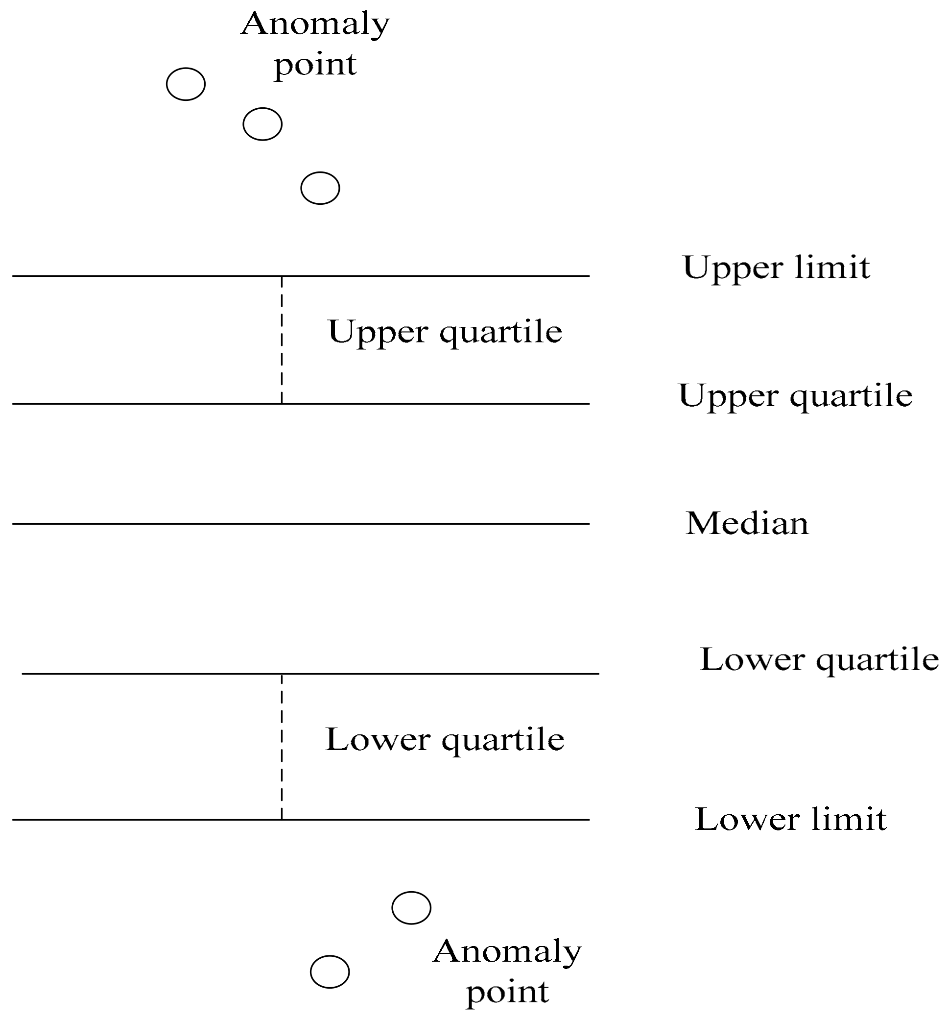
As shown in Figure 6, the box diagram is a method for determining the final result. The upper and lower abnormal boundary values are continuously monitored online, and the data are labeled as abnormal by focusing on the data exceeding the upper limit and lower limit curves. The advantage of this analysis method is that it can increase the judgment margin.
On the basis of satisfying the concept drift, it can adapt to the change of parameters in real time, track the dynamic trend of the data stream, and, also in real time, monitor and classify the data in the sliding window. On the basis of satisfying the data stream, it meets the analysis requirements of sliding window technology.
4. Simulation and Comparison
The data selected in this paper is the drilling data of the Tarim oilfield. The oil drilling data is a typical industrial data stream. There are dozens of sensors at the drilling site, and the parameters, including the derived parameters, are between 100 and 300 parameters. Affected by the sensor installation position, performance, and working environment, data stream data are often interrupted and lost. The sampling frequency of these data streams is generally 1 or 0.2 Hz. The sampling frequency chosen in this paper is 1 Hz. The analysis parameter is the total cell volume. The comparison algorithms are the automatic outlier detection for data streams (A-ODDS) [30,31] and SNWCAD-DS algorithms. The adopted standard is the area under the curve (AUC) and the Jaccard similarity coefficient. The specific object of analysis consists of 1413 total pool volume data, which is firstly tagged with expert experience, and then, supervised classification methods are applied to these tagged data. The accuracy and false positive rate are tested by comparing different algorithms, and the quality of the algorithm is thus determined. The complexity of the algorithm is based on the same data analysis length comparison. The algorithm comparison formula is as follows:
If a positive class tag is predicted to be negative, it is called false negative (FN); if the negative class tag is predicted to be negative, it is called true negative (TN); if the negative class tag is predicted to be positive, it is called false positive (FP); and, if a positive class tag is predicted to be positive, it is called true positive (TP). In addition, the AUC is calculated by changing the threshold, so is considered as a threshold. True positive rate (TPR) is the accuracy rate, and false positive rate (FPR) is the false alarm rate.
Jaccard’s coefficient is expressed as follows:
The higher Jaccard’s coefficient (JC), the higher the similarity. The receiver operating characteristic (ROC) comprises two categories: anomaly data and normal data. In the anomaly data, we not only identify abnormal rises but also identify abnormal declines. Therefore, it considers three categories in total.
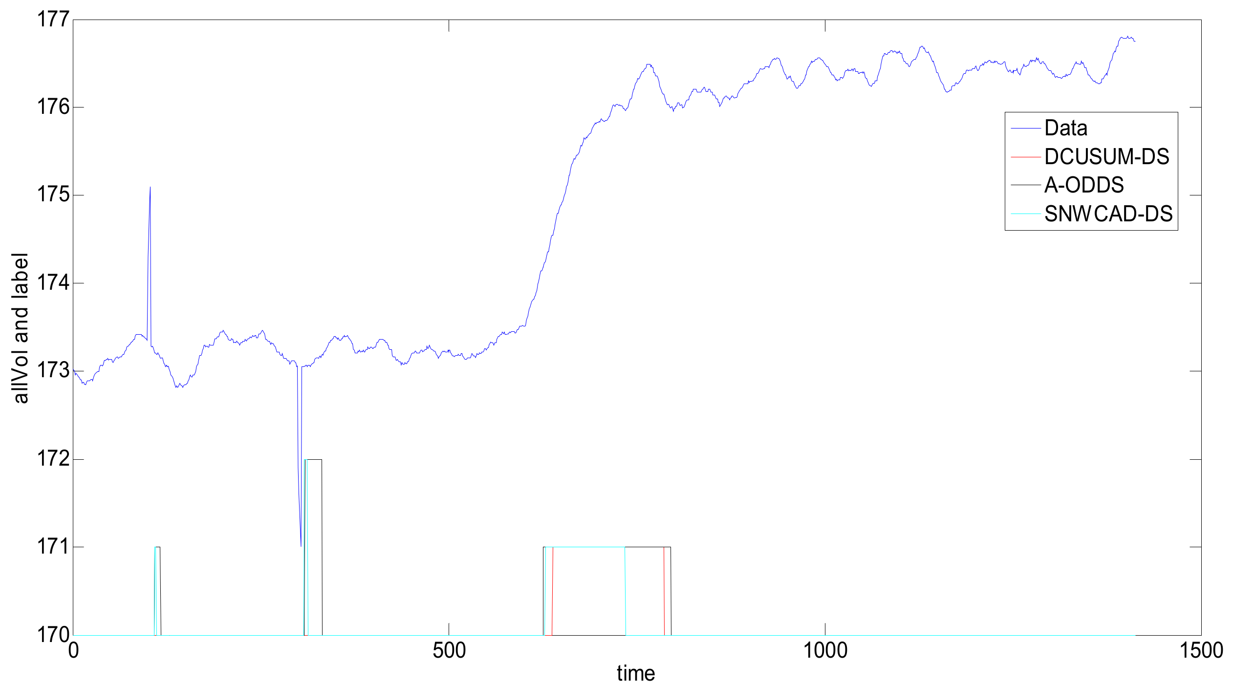
As shown in Figure 7, there are four points that show an upward trend and that deviate from the normal trend at 100, and five points that have a downward trend and that deviate from the normal trend at 300.
The difficulty in data stream anomaly monitoring is that the data stream is infinitely accumulating. When the current point deviating from the normal trend enters the sliding window, it is necessary to refer to not only the data value of the current moment, but also the values of several data that are close and that have also deviated from normal trends in the past few moments. As shown in the above figure, at the interference points at 100 and 300 on the time axis, the traditional data stream machine learning is often misclassified. The interference on the time axis 100 are abnormally rising, and the interference on the time axis 300 are abnormally low; these phenomena are ubiquitous in engineering. In this case, such classification is wrong because, at these two moments, there are no associated accidents or targets. The cause of this data change may be environmental interference or the sensor installation location. The purpose of the newly designed DCUSUM-DS algorithm is to detect the abnormal upward trend of the data stream after 600, to mark 600–700 data points as rising labels, to shield the interference of some points deviations, and to label the interference data as normal.
As shown in Table 1, in order to improve the fairness and credibility of each algorithm’s detection accuracy, the false alarm rate, and the algorithm complexity, the same parameters are set for each algorithm. The long window is uniformly set to 140, the short window is set to 25, the threshold is set to 0.5, and the outbound rate is set to 8. The following simulation, in addition to the data listed in Table 2, uses the parameter settings in Table 1 and compares the advantages and disadvantages of each algorithm by comparing the TPR, FPR, the AUC area, and the algorithm calculation time.
As shown in Figure 8, the abnormal rising flag is 1, and the abnormal falling flag is 2. Through the simulation comparison of the three methods, we can see that the DCUSUM-DS can not only detect the abnormal increase of the data stream at 600–700 points but can also shield the interference of a few data at 100 and 300, achieving the purpose of the design and meeting the actual needs of the site. Although the A-ODDS and SNWCAD-DS algorithms can detect the abnormal increase of data streams at 600–700, 100 and 300 interference data cannot be masked. Therefore, the new proposed algorithm DCUSUM-DS achieves its purpose.
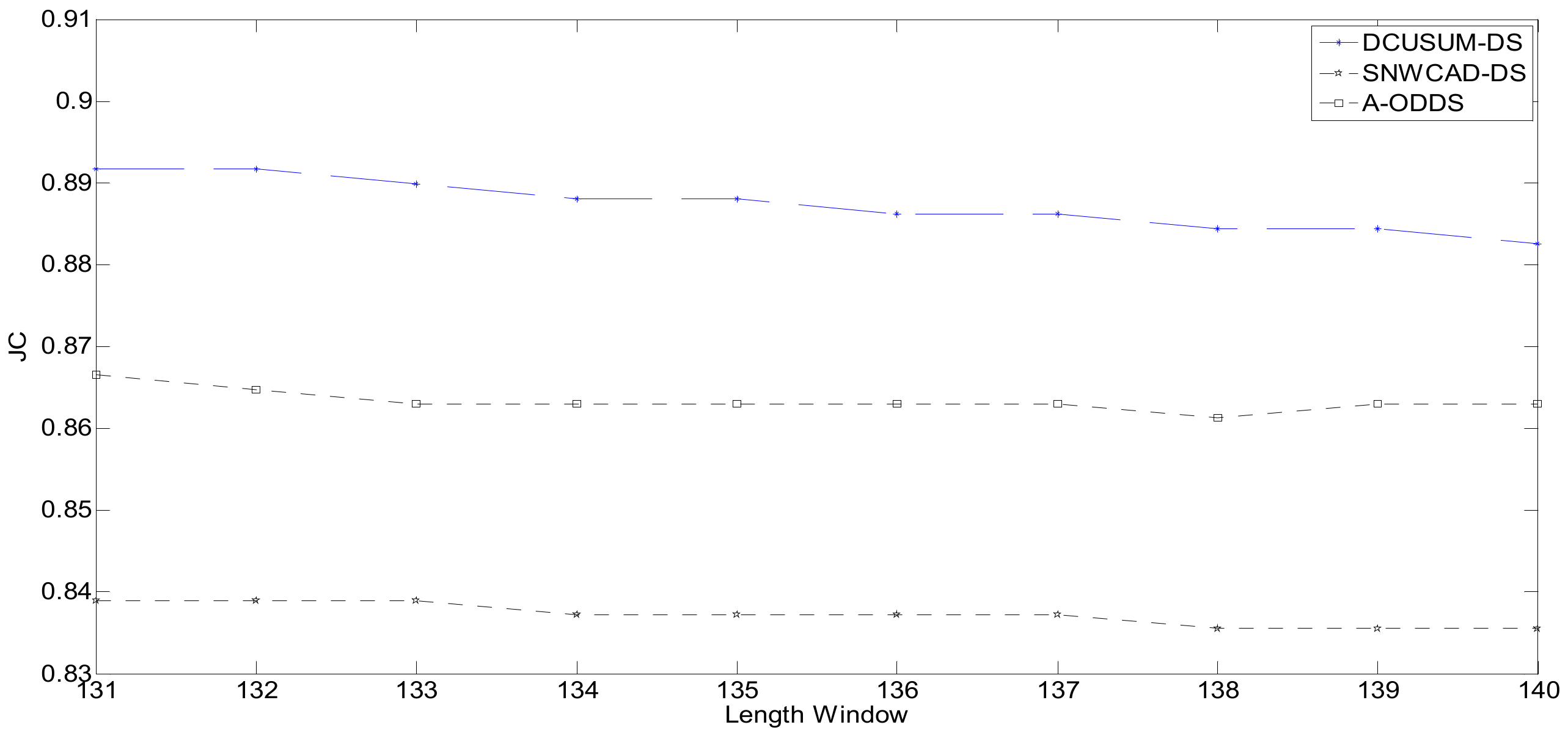
Figure 9 shows the distribution of Jaccard’s coefficient. The abscissa is the length of the long window. The meaning of this expression is to obtain different Jaccard’s coefficients by setting different lengths of the window and to obtain Jaccard’s coefficient through different window lengths to analyze and compare the quality of the algorithm. Jaccard’s coefficient represents a similarity measure of the online stream classification algorithm for data stream machine learning.
The factors affecting Jaccard’s coefficient include not only the correct rate of the classification result, the error rate, and the missing report rate, but also the setting of the window length and the outbound rate. Due to the delay, the higher Jaccard’s coefficient, the higher the accuracy; the lower Jaccard’s coefficient, the lower the accuracy. The operating environment involves the Central Processing Unit (CPU) dual-core 2.1GHz, Win7 Sp1 x86, and memory 2G. The running time is shown in Table 2.
Table 2 is a further interpretation of Figure 9. The table shows the time of each single-step analysis for different lengths of the long window and objectively evaluates the complexity of the algorithm by averaging the time. The calculated operating environment is as follows: Win7 Sp1 x86, a CPU dual-core 2.1 GHz, 2G memory. According to the sampling frequency of 1 Hz, the proposed new algorithm can be calculated within 0.2 s in a 1 s interval, which fully meets the actual operating requirements of the site.
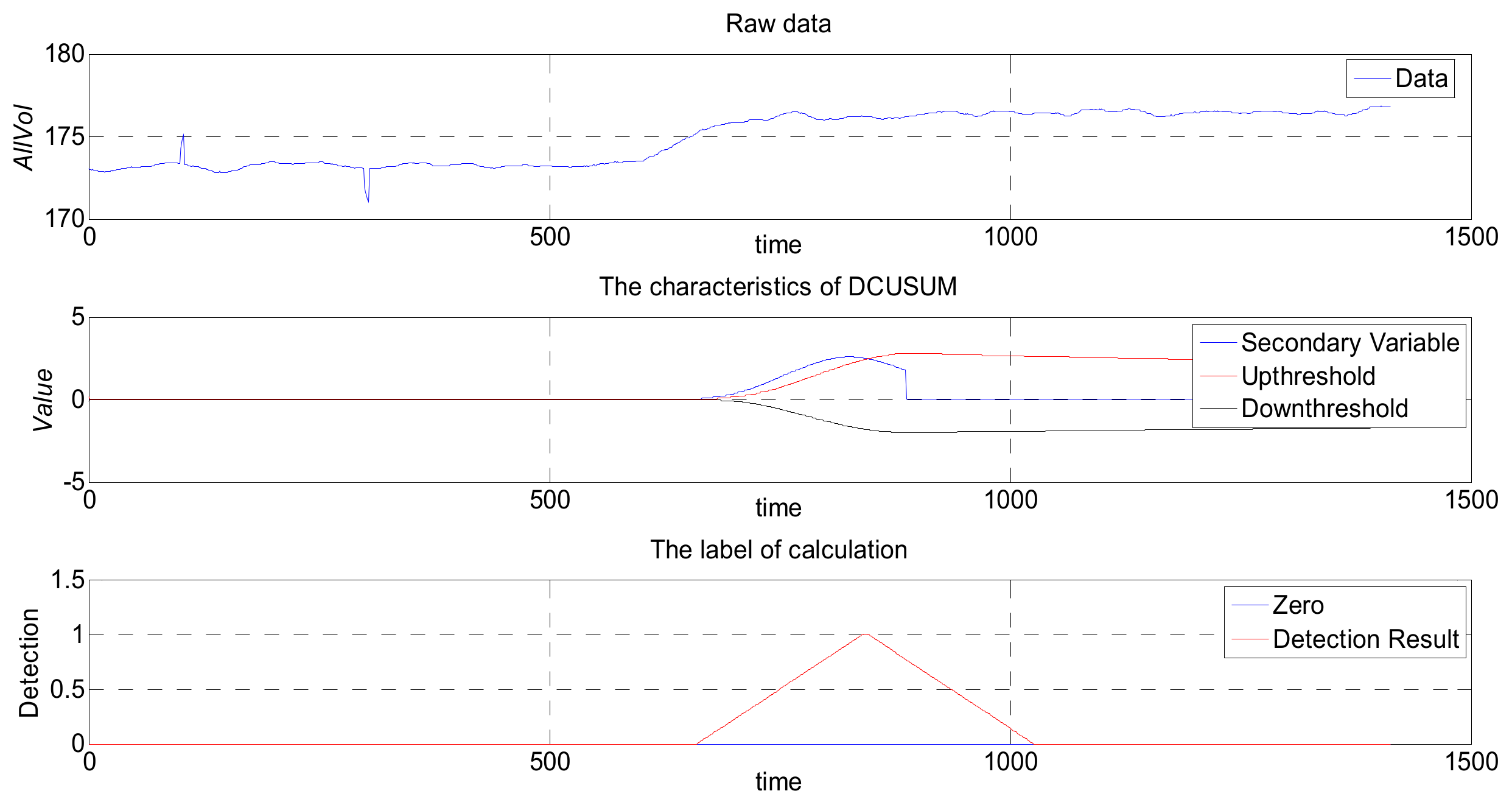
As shown in Figure 10, the data in the normal range are enveloped in the upper and lower threshold lines. When there is an abnormal rise or an abnormal drop, the feature value will exceed the threshold line. The anomaly detection algorithm deals with the current point and several nearby data. After the cumulative number of deviation data exceeds the set demarcation rate, the anomaly detection algorithm reaches the classification criteria. Afterward, the abnormal points that continue this trend are labeled as abnormal data, and the previous abnormal points are labeled as normal data.
Figure 11 maps the original values of the DCUSUM-DS space. The top graph is drawn from the original data, the middle graph is the feature quantity graph after data conversion, and the bottom graph is the tagged data graph. It can be clearly seen from the middle graph that the feature amount obviously exceeds the upper threshold line. The bottom graph clearly shows that the original data have a significant anomaly, while the other two interference points are not displayed, which is consistent with the original intention of the algorithm design.
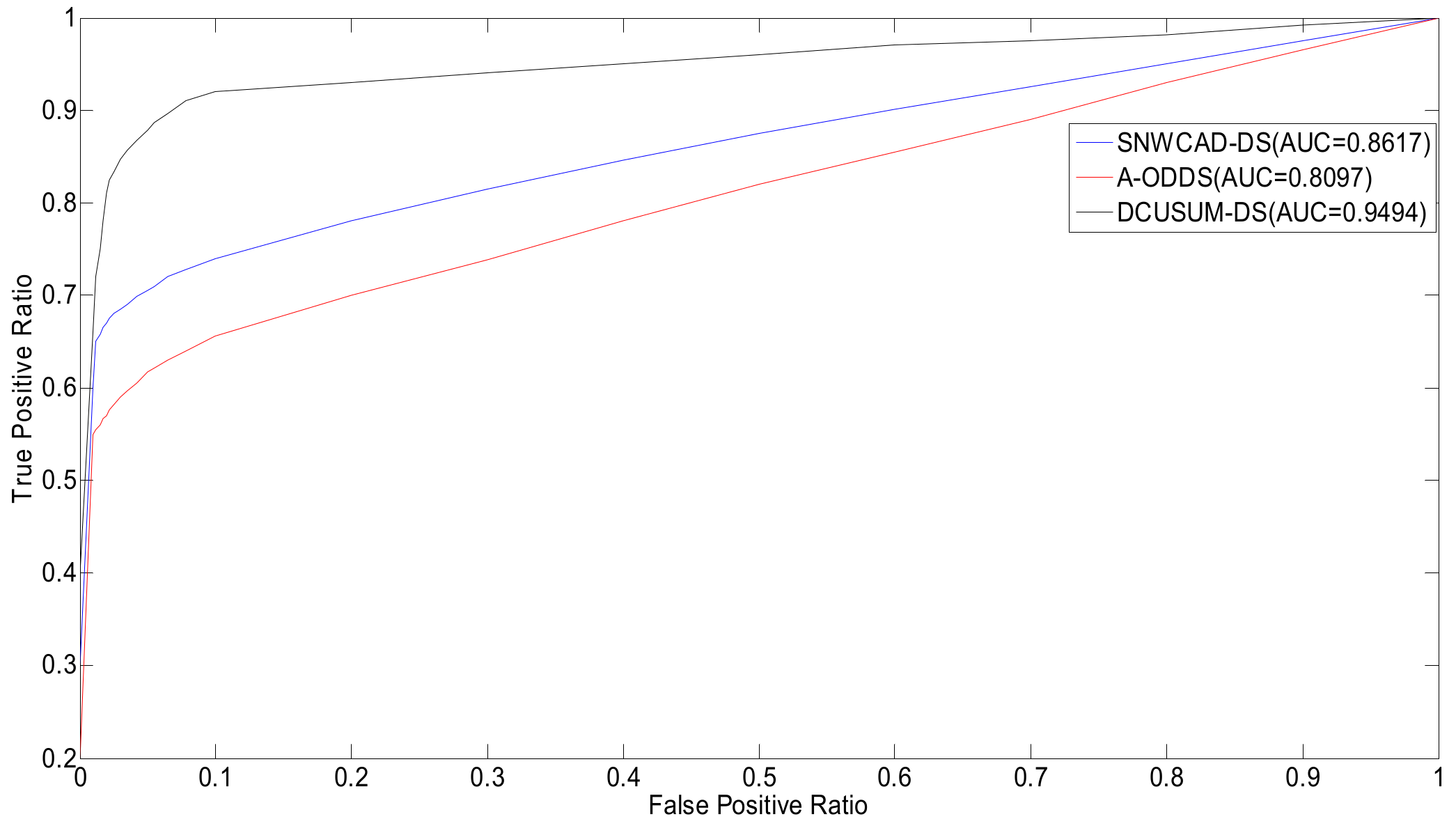
Figure 12 indicates that the proposed new algorithm DCUSUM can increase the TPR and reduce the FPR, compared with SNWCAD-DS and A-ODDS.
Through analysis of Figure 9, Figure 12, and Table 2, we can conclude that the proposed new algorithm DCUSUM-DS improves the accuracy of online classification and reduces the misclassification rate. The influence of the interference data can be masked, real abnormal data can be detected, and the interference data can be filtered out. Computational complexity does not significantly increase, and the algorithm fully meets the relevant working requirements. The laboratory simulation and field application show that the algorithm solves the machine classification problems that arise from poor data quality in industrial data streams, thus improving machine learning classification.
5. Summary
This paper proposes the DCUSUM algorithm to determine the effect of interference data on the classification of industrial data streams. This algorithm is further processed on the basis of the SNWCAD-DS algorithm to improve the classification of the industrial data stream affected by interference data. The contributions of this work can be concluded as follows: (1) DCUSUM-DS can block misclassification problems caused by points that deviate from normal trends and can improve the problem of low detection efficiency caused by the classification of traditional data; (2) Compared with A-ODDS and SNWCAD-DS, DCUSUM-DS can improve detection accuracy; and (3) The computational complexity of DCUSUM-DS meets the practical needs of field engineering and meets all relevant engineering requirements.
In the future, research on each parameter in the algorithm, such as the length of the sliding window, needs to be carried out. Furthermore, the robustness and applicability of the algorithm need to be verified.
Author Contributions
G.L. and C.Y. conceived of and designed the experiments; G.L. performed the experiments and analyzed the data; and J.W. and J.L. provided guidance and recommendations for this research. G.L. contributed to the contents and writing of this manuscript.
Funding
The National Natural Science Foundation of China (61473266 and 61673404), the Research Award Fund for Outstanding Young Teachers in Henan Provincial Institutions of Higher Education of China (2014GGJS-004), and the Program for Science & Technology Innovation Talents in Universities of Henan Province in China (16HASTIT041) for financial support.
Conflicts of Interest
The authors declare no conflicts of interest.
References
- Li, G.; Zhang, H.; Wang, J.; Zhu, X.D.; Yue, C.T. A review: Pre-warning system of oil-drilling engineering. J. Zhengzhou Univ. (Eng. Sci.) 2017, 38, 70–73. [Google Scholar]
- Li, G.; Wang, J.; Liang, J.; Yue, C. Application of sliding nest window control chart in data stream anomaly detection. Symmetry 2018, 10, 113. [Google Scholar] [CrossRef]
- Siddique, K.; Akhtar, Z.; Lee, H.G.; Kim, W.; Kim, Y. Toward Bulk Synchronous Parallel-Based Machine Learning Techniques for Anomaly Detection in High-Speed Big Data Networks. Symmetry 2017, 9, 197. [Google Scholar] [CrossRef]
- Zabihi, M.; Rad, A.B.; Kiranyaz, S.; Gabbouj, M.; Katsaggelos, A.K. Heart Sound Anomaly and Quality Detection using Ensemble of Neural Networks without Segmentation. In Proceedings of the 2016 Computing in Cardiology Conference (CinC), Vancouver, BC, Canada, 11–14 September 2016; pp. 613–616. [Google Scholar]
- Li, F.; Wang, H.; Zhou, G.; Yu, D.; Li, J.; Gao, H. Anomaly Detection in Gas Turbine Fuel Systems Using a Sequential Symbolic Method. Energies 2017, 10, 724. [Google Scholar] [CrossRef]
- Lan, K.; Fong, S.; Song, W.; Vasilakos, A.V.; Millham, R.C. Self-Adaptive Pre-Processing Methodology for Big Data Stream Mining in Internet of Things Environmental Sensor Monitoring. Symmetry 2017, 9, 244. [Google Scholar] [CrossRef]
- Gil, A.; Sanz-Bobi, M.A.; Rodríguez-López, M.A. Behavior Anomaly Indicators Based on Reference Patterns—Application to the Gearbox and Electrical Generator of a Wind Turbine. Energies 2018, 11, 87. [Google Scholar] [CrossRef]
- Costa, F.G.D.; Duarte, F.S.L.G.; Vallim, R.M.M.; de Mello, R.F. Multidimensional Surrogate stability to Detect Data Stream Concept Drift. Expert Syst. Appl. 2017, 87, 15–29. [Google Scholar] [CrossRef]
- Ramírez-Gallego, S.; Krawczyk, B.; García, S.; Woźniak, M.; Herrera, F. A Survey on Data Preprocessing for Data Stream Mining: Current Status and Future Directions. Neurocomputing 2017, 239, 39–57. [Google Scholar] [CrossRef]
- Jankov, D.; Sikdar, S.; Mukherjee, R.; Teymourian, K.; Jermaine, C. Real-time High Performance Anomaly Detection over Data Streams: Grand Challenge. In Proceedings of the 11th ACM International Conference on Distributed and Event-Based Systems, Barcelona, Spain, 19–23 June 2017; pp. 292–297. [Google Scholar]
- Simão, M.A.; Neto, P.; Gibaru, O. Unsupervised Gesture Segmentation by Motion Detection of a Real-Time Data Stream. IEEE Trans. Ind. Inf. 2017, 13, 473–481. [Google Scholar] [CrossRef]
- Zhang, L.; Lin, J.; Karim, R. Sliding Window-based Fault Detection from High-dimensional Data Streams. IEEE Trans. Syst. Man Cybern. Syst. 2017, 47, 289–303. [Google Scholar] [CrossRef]
- Tran, K.P.; Castagliola, P.; Celano, G. Monitoring the Ratio of Population Means of a Bivariate Normal Distribution Using CUSUM type Control Charts. Stat. Pap. 2018, 59, 387–413. [Google Scholar] [CrossRef]
- Rafaelof, M.; Mustak, H.; Rootman, D.B. Anomalous Sphenoid Diploe Vein: Case Report Highlighting the Value of Careful CT Evaluation Prior to Decompression Surgery. Ophthalmic Plast. Reconstr. Surg. 2018, 34, 74–75. [Google Scholar] [CrossRef] [PubMed]
- Liang, P.; Yang, H.D.; Chen, W.S.; Xiao, S.Y.; Lan, Z.Z. Transfer Learning for Aluminium Extrusion Electricity Consumption Anomaly Detection Via Deep Neural Networks. Int. J. Comput. Integr. Manuf. 2018, 31, 396–405. [Google Scholar] [CrossRef]
- Aytekin, C.; Ni, X.; Cricri, F.; Aksu, E. Clustering and Unsupervised Anomaly Detection with L2 Normalized Deep Auto-Encoder Representations. arXiv, 2018; arXiv:1802.00187. [Google Scholar]
- Khan, S.; Gani, A.; Wahab, A.W.A.; Singh, P.K. Feature selection of Denial-of-Service attacks using entropy and granular computing. Arab. J. Sci. Eng. 2018, 43, 499–508. [Google Scholar] [CrossRef]
- Li, G.; Wang, J.; Liang, J.; Yue, C.; Fan, Y.; Song, D.; Lv, Z. Study on drilling engineering prewarning based on random forests. J. Oil Gas Technol. 2017, 39, 193–198. [Google Scholar] [CrossRef]
- Youn, I.H.; Youn, J.H.; Lee, J.M.; Kim, C.S. Anomaly event Detection for sit-to-stand Transition Recognition to improve Mariner Physical activity Classification during a Sea Voyage. Biomed. Res. 2018, 29, 444–447. [Google Scholar] [CrossRef]
- Sun, Y.; Tang, K.; Minku, L.L.; Wang, S.; Yao, X. Online Ensemble Learning of Data Streams with Gradually Evolved classes. IEEE Trans. Knowl. Data Eng. 2016, 28, 1532–1545. [Google Scholar] [CrossRef]
- Jung, I.S.; Berges, M.; Garrett, J.H.; Poczos, B. Exploration and evaluation of AR, MPCA and KL anomaly detection techniques to embankment dam piezometer data. Adv. Eng. Inf. 2015, 29, 902–917. [Google Scholar] [CrossRef] [Green Version]
- Lang, M. A Low-Complexity Model-Free Approach for Real-Time Cardiac Anomaly Detection Based on Singular Spectrum Analysis and Nonparametric Control Charts. Technologies 2017, 15, 26. [Google Scholar]
- Widmer, G.; Kubat, M. Learning in the presence of concept drift and hidden contexts. Mach. Learn. 1996, 23, 69–101. [Google Scholar] [CrossRef] [Green Version]
- Ahn, K.; Cormode, G.; Guha, S.; McGregor, A.; Wirth, A. Correlation Clustering in Data Streams. In Proceedings of the International Conference on Machine Learning, Lille, France, 6–11 July 2015; pp. 2237–2246. [Google Scholar]
- Chen, Q.; Chen, L.; Lian, X.; Liu, Y.; Yu, J.X. Indexable PLA for Efficient Similarity Search. In Proceedings of the 33rd International Conference on Very Large Data Bases, Vienna, Austria, 23–27 September 2007; pp. 435–446. [Google Scholar]
- Liu, X.; Guan, J.; Hu, P. Mining frequent closed itemsets from a landmark window over online data streams. Comput. Math. Appl. 2009, 57, 927–936. [Google Scholar] [CrossRef] [Green Version]
- Babcock, B.; Babu, S.; Datar, M.; Motwani, R.; Widom, J. Models and issues in data stream systems. In Proceedings of the Twenty-First ACM SIGMOD-SIGACT-SIGART Symposium on Principles of Database Systems, Madison, WI, USA, 3–5 June 2002; pp. 1–16. [Google Scholar]
- Huang, Y.; Tang, J.; Cheng, Y.; Li, H.; Campbell, K.A.; Han, Z. Real-time Detection of False Data Injection in smart Grid Networks: An adaptive CUSUM Method and Analysis. IEEE Syst. J. 2016, 10, 532–543. [Google Scholar] [CrossRef]
- Cordeschi, N.; Shojafar, M.; Amendola, D.; Baccarelli, E. Energy-saving QoS resource management of virtualized networked data centers for Big Data Stream Computing. In Big Data: Concepts, Methodologies, Tools, and Applications; IGI Global: Hershey, PA, USA, 2016; pp. 848–886. [Google Scholar]
- Baccarelli, E.; Cordeschi, N.; Mei, A.; Panella, M.; Shojafar, M.; Stefa, J. Energy-efficient dynamic traffic offloading and reconfiguration of networked data centers for big data stream mobile computing: Review, challenges, and a case study. IEEE Netw. 2016, 30, 54–61. [Google Scholar] [CrossRef]
- Sadik, S.; Le, G. An adaptive Outlier Detection Technique for Data Streams. In Proceedings of the International Conference on Scientific and Statistical Database Management, Portland, OR, USA, 20–22 July 2011; pp. 596–597. [Google Scholar]
Figure 1.
Decision process of the data stream.

Figure 2.
Schematic diagram of the pending problem.
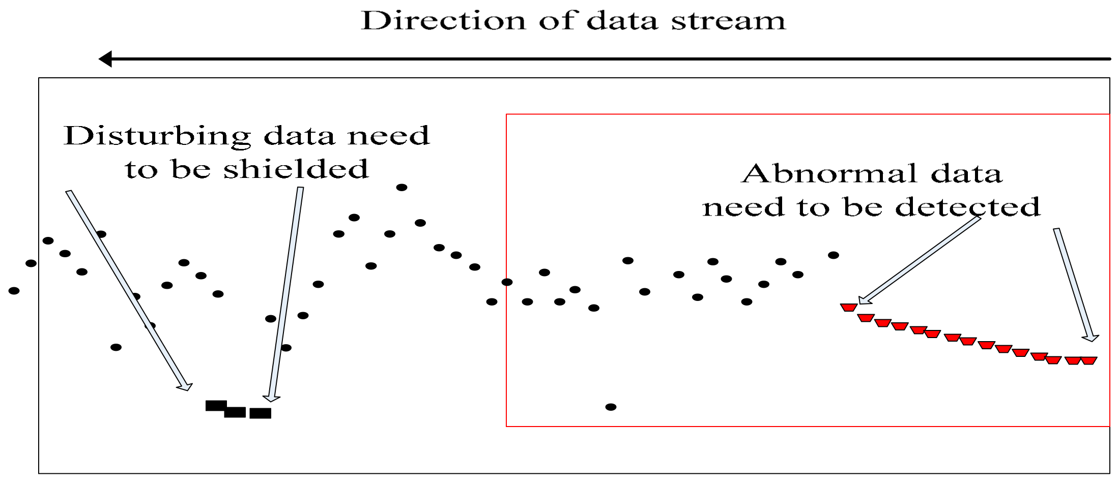
Figure 3.
Different kinds of window methods.

Figure 4.
Schematic diagram of the working principle of cumulative sum (CUSUM).
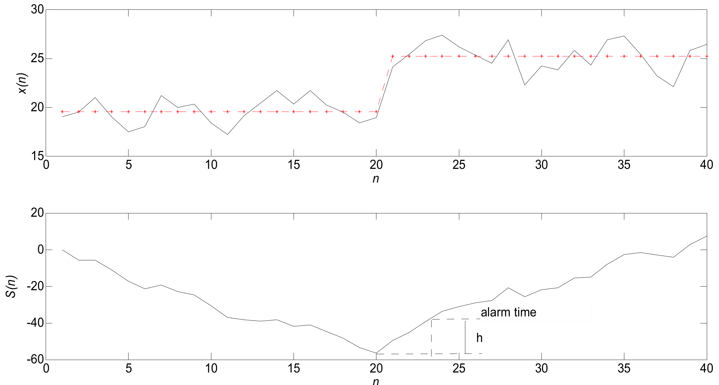
Figure 5.
Algorithm flowchart of DCUSUM-DS.
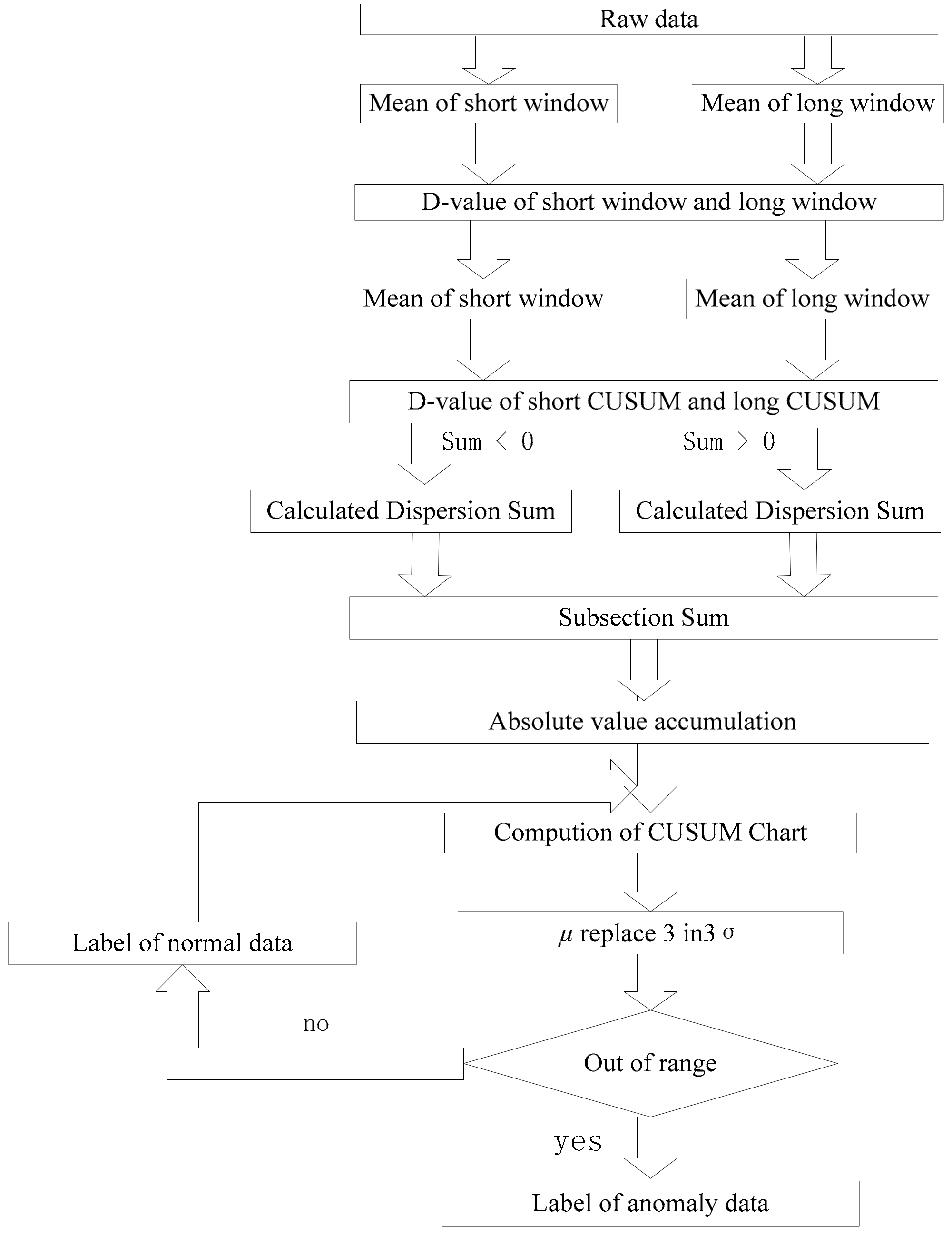
Figure 6.
Parameters of the box plot.

Figure 7.
Drilling engineering torque data.
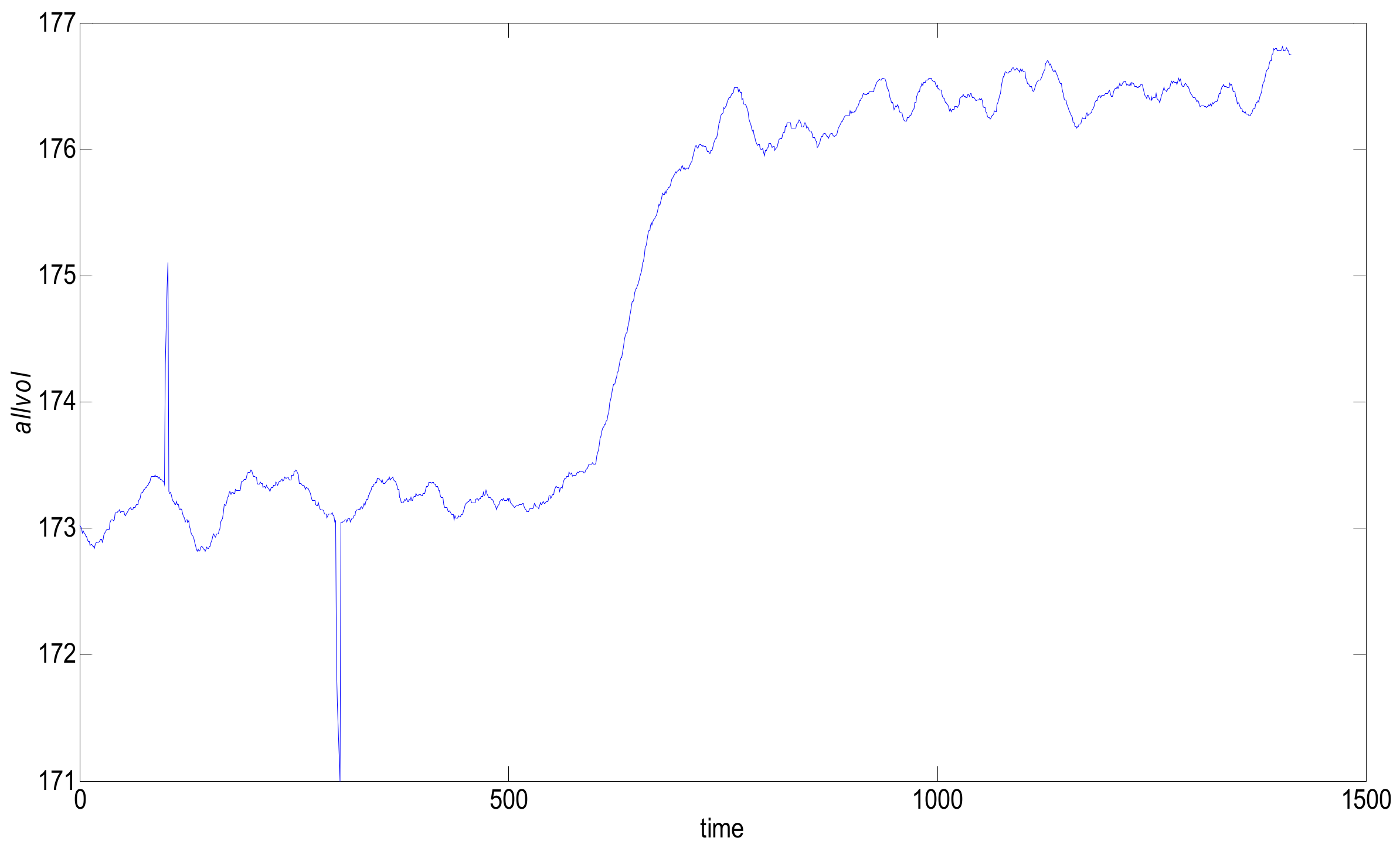
Figure 8.
Comparison of classification results of various data stream machine learning algorithms.

Figure 9.
Jaccard’s coefficient of each algorithm.

Figure 10.
Data analysis diagram of DCUSUM.

Figure 11.
Feature space mapping of DCUSUM.

Figure 12.
Comparison of receiver operating characteristic (ROC) and area under the curve (AUC) of various data stream machine learning algorithms.
Figure 12.
Comparison of receiver operating characteristic (ROC) and area under the curve (AUC) of various data stream machine learning algorithms.


Table 1.
Algorithm setting table.
| Algorithm | Length of Short Window | Length of Long Window | Threshold | Out Rate |
|---|---|---|---|---|
| DCUSUM-DS | 25 | 140 | 0.5 | 8 |
| SNWCAD-DS | 25 | 140 | 0.5 | 8 |
| A-ODDS | 25 | 140 | 0.5 | / |
Table 2.
Computational complexity comparison.
| Setting of Long Window | DCUSUM-DS | A-ODDS | SNWCAD-DS |
|---|---|---|---|
| 131 | 0.1812 | 0.0867 | 0.0912 |
| 132 | 0.1821 | 0.0871 | 0.0919 |
| 133 | 0.1823 | 0.0875 | 0.0924 |
| 134 | 0.1826 | 0.0879 | 0.0932 |
| 135 | 0.1833 | 0.0931 | 0.1041 |
| 136 | 0.1839 | 0.0939 | 0.1085 |
| 137 | 0.1841 | 0.0944 | 0.1167 |
| 138 | 0.1846 | 0.0952 | 0.1174 |
| 139 | 0.1853 | 0.0959 | 0.1181 |
| 140 | 0.1859 | 0.0963 | 0.1190 |
| Average | 0.18353 | 0.0918 | 0.10525 |
© 2018 by the authors. Licensee MDPI, Basel, Switzerland. This article is an open access article distributed under the terms and conditions of the Creative Commons Attribution (CC BY) license (http://creativecommons.org/licenses/by/4.0/).
Share and Cite
MDPI and ACS Style
Li, G.; Wang, J.; Liang, J.; Yue, C. The Application of a Double CUSUM Algorithm in Industrial Data Stream Anomaly Detection. Symmetry 2018, 10, 264. https://doi.org/10.3390/sym10070264
AMA Style
Li G, Wang J, Liang J, Yue C. The Application of a Double CUSUM Algorithm in Industrial Data Stream Anomaly Detection. Symmetry. 2018; 10(7):264. https://doi.org/10.3390/sym10070264
Chicago/Turabian StyleLi, Guang, Jie Wang, Jing Liang, and Caitong Yue. 2018. "The Application of a Double CUSUM Algorithm in Industrial Data Stream Anomaly Detection" Symmetry 10, no. 7: 264. https://doi.org/10.3390/sym10070264
Note that from the first issue of 2016, this journal uses article numbers instead of page numbers. See further details here.