Iterative Group Decomposition for Refining Microaggregation Solutions


1
Faculty of Management Science, Nakhon Ratchasima Rajabhat University, Nakhon Ratchasima 30000, Thailand
2
Department of Information Management, Yuan Ze University, Taoyuan 32003, Taiwan
3
Innovation Center for Big Data and Digital Convergence, Yuan Ze University, Taoyuan 32003, Taiwan
*
Author to whom correspondence should be addressed.
Symmetry 2018, 10(7), 262; https://doi.org/10.3390/sym10070262
Submission received: 28 May 2018
/
Revised: 17 June 2018
/
Accepted: 2 July 2018
/
Published: 4 July 2018
(This article belongs to the Special Issue Information Technology and Its Applications 2021)
Abstract
:Microaggregation refers to partitioning n given records into groups of at least k records each to minimize the sum of the within-group squared error. Because microaggregation is non-deterministic polynomial-time hard for multivariate data, most existing approaches are heuristic based and derive a solution within a reasonable timeframe. We propose an algorithm for refining the solutions generated using the existing microaggregation approaches. The proposed algorithm refines a solution by iteratively either decomposing or shrinking the groups in the solution. Experimental results demonstrated that the proposed algorithm effectively reduces the information loss of a solution.
1. Introduction
Protection of publicly released microdata from individual identification is a primary societal concern. Therefore, statistical disclosure control (SDC) is often applied to microdata before releasing the data publicly [1,2]. Microaggregation is an SDC method, which functions by partitioning a dataset into groups of at least k records each and replacing the records in each group with the centroid of the group. The resulting dataset satisfies the “k-anonymity constraint,” thus protecting data privacy [3]. However, replacing a record with its group centroid results in information loss, and the amount of information loss is commonly used to evaluate the effectiveness of a microaggregation method.
A constrained clustering problem underlies microaggregation, in which the objective is to minimize information loss and the constraint is to restrict the size of each group of records to not fewer than k. This problem can be solved in polynomial time for univariate data [4]; however, it has been proved non-deterministic polynomial-time hard for multivariate data [5]. Therefore, most existing approaches for multivariate data are heuristic based and derive a solution within a reasonable timeframe; consequently, no single microaggregation method outperforms other methods for all datasets and k values.
Numerous microaggregation methods have been proposed, e.g., the Maximum Distance to Average Vector (MDAV) [6], Diameter-Based Fixed-Size (DBFS) [7], Centroid-Based Fixed-Size (CBFS) [7], Two Fixed Reference Points (TFRP) [8], Multivariate Hansen–Mukherjee (MHM) [9], Density-Based Algorithm [10], Successive Group Minimization Selection (GSMS) [11], and Fast Data-oriented Microaggregation [12]. They generate a solution that satisfies the k-anonymity constraint and minimizes the information loss for a given dataset and an integer k. A few recent studies have focused on refining the solutions generated using existing microaggregation methods [13,14,15,16]. The most widely used method for refining a microaggregation solution is to determine whether decomposing each group of records in the solution by adding its records to other groups can reduce the information loss of the solution. This method, referred to as TFRP2 in this paper, is originally used in the second phase of the TFRP method [8] and has been subsequently adopted by many microaggregation approaches [10,11].
Because the above microaggregation approaches are based on simple heuristics and do not always yield satisfactory solutions, there is room to improve the results of these existing approaches. Our aim here is to develop an algorithm for refining the results of the existing approaches. The developed algorithm should help the existing approaches to reduce the information loss further.
The remainder of this paper is organized as follows. Section 2 defines the microaggregation problem. Section 3 reviews relevant studies on microaggregation approaches. Section 4 presents the proposed algorithm for refining a microaggregation solution. The experimental results are discussed in Section 5. Finally, conclusions are presented in Section 6.
2. Microaggregation Problem
Consider a dataset D of n points (records), xi, i∈{1,…,n}, in the d-dimensional space. For a given positive integer k ≤ n, the microaggregation problem is to derive a partition P of D, such that |p| ≥ k for each group p∈P and SSE(P) is minimized. Here, SSE(P) denotes the sum of the within-group squared error of all groups in P and is calculated as follows:
The information loss incurred by the partition P is denoted as IL(P) and is calculated as follows:
Because SST(D) is fixed for a given dataset D, regardless of how D is partitioned, minimizing SSE(P) is equivalent to minimizing . Furthermore, if a group contains 2k or more points, it can be split into two or more groups, each with k or more points, to reduce information loss. Thus, in an optimal partition, each group contains at most 2k − 1 points [17].
This study proposed an algorithm for refining the solutions generated using the existing microaggregation methods. The algorithm reduces the information loss of a solution by either decomposing or shrinking a group in the solution. Experimental results obtained using the standard benchmark datasets show that the proposed algorithm effectively improves the solutions generated using state-of-the-art microaggregation approaches.
3. Related Work
3.1. Microaggregation Approaches
Many microaggregation approaches are based on a fixed-size heuristics in which groups of size k are iteratively built around the selected records [6,7,8,10,11]. These approaches mainly differ in two aspects: selection of the first record for each group and formation of a group of size k from the selected record.
Let T denote the remaining unpartitioned records in D. Initially, T = D. Common methods to choose from T for the first record of a new group are as follows: the record (denoted as r) furthest from the centroid of T (e.g., MDAV [6] and CBFS [7]), the record furthest from r (e.g., MDAV [6]), the two records in T most distant from each other (e.g., DBFS [7]), and the two records furthest from the two fixed reference points of D (e.g., TFRP [8]), where the reference points are separately determined from the maximal and minimal values over all attributes in D.
Once the first record of a group is determined, one of the following two methods is commonly adopted to grow the group to size k. The first method (referred to as Nearest Neighbors and denoted as NN) is to form a group with the selected record and its k − 1 nearest neighbors in T [6,8,10,11]. The other (referred as Nearest to Center and denoted as NC) is to iteratively update the centroid of the group and add the record in T that is nearest to the centroid of the group until the size of the group reaches k [7]. The first method is faster, whereas the second is inclined towards minimizing the SSE of the generated group.
GSMS [11], a fixed-size approach, adopts a different approach to iteratively build groups of size k. Instead of choosing a record and then forming a group, it forms a candidate group for each record in T by using the record and its k − 1 nearest records. Subsequently, the candidate group p with the smallest SSE(p) + SSE(T/p) is selected, where T/p denotes the difference of T and p. A priority queue is maintained for each record in T to update all candidate groups rapidly. However, such an arrangement could result in high space complexity.
To speed up the fixed-size approaches, one can either use an efficient way to pick the first record of each group [18,19,20] or reduce the size of the dataset to be processed [21]. In Refs. [18,19,20], the authors first sorted all records by an auxiliary attribute. To build a new group, they used the first unassigned record in this ordering as the first record of the new group, and then grew the new group to size k by adding the first record’s k − 1 nearest neighbors. In Ref. [21], the authors first selected several attributes that have a high mutual information measure with other attributes. Then, they applied MDAV on the projection of the dataset on those selected attributes. Finally, the partition results were extended to all attributes to calculate each group’s centroid.
In addition to fixed-size heuristics, many microaggregation approaches were derived using methods not originally designed for the multivariate microaggregation problem. For example, MDAV–MHM [9] first adopted heuristics (e.g., MDAV) to order the multivariate records and then used Hansen–Mukherjee method (a microaggregation approach for univariate data [4]) to partition the data according to this ordering. Other examples include Ref. [7] and Ref. [22], which extended the minimal spanning tree partitioning algorithm [23], and Ref. [17], which extended Ward’s agglomerative hierarchical clustering algorithm [24] to the microaggregation problem.
In this work, we focused on the k-anonymity constraint. However, many extensions of the k-anonymity appeared in the literature, e.g., l-diversity [25], t-closeness [26] and (k, ϵ, l)-anonymity [27]. Ref. [28] proposed a microaggregation method to steer the microaggregation process such that the desired privacy constraints were satisfied.
3.2. Refining Approaches
Most approaches for refining a microaggregation solution involved iteratively generating new solutions and searching for possible improvements [13,14,15,16]. Clustering algorithms, such as k-means and h-means, were adopted in [13] to modify a microaggregation solution. This approach used a pattern search algorithm to search for the appropriate value of a parameter.
Iterative MHM, proposed in Ref. [14], built groups of a microaggregation solution according to constrained clustering and linear programming relaxation and then fine-tuned the results using an integrated iterative approach. Its solution was built on the microaggregation solution generated using the MDAV method, and the number of groups in the solution was determined in the same manner as in MDAV-MHM [9].
An iterative local search approach [15] was proposed to refine a microaggregation solution. During the local search, the microaggregation solution was improved by swapping a record between two groups and shifting a record from one group to another. Furthermore, to explore the results using a different number of groups, the number of groups in a solution was updated randomly within an optimal range in each iteration. In addition, the “dissolve” operation (same as the TFRP2 method described in Section 1) and the “distill” operation (i.e., forming a new group by removing records from groups with more than k records) were used to adjust the number of groups in the solution.
Similar to Ref. [15], another iterative local search approach proposed in [16] used swapping and shifting of the records between two groups to refine a microaggregation solution. This method expanded the search space by allowing more than one swapping or shifting in each iteration of the local search.
4. Proposed Algorithm
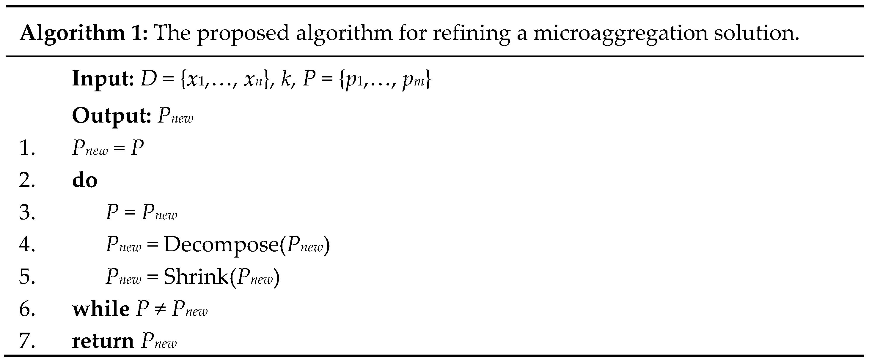
Figure 1 shows the pseudocode of the proposed algorithm for refining a microaggregation solution. The input to the algorithm is a partition P of a dataset D generated using a fixed-size microaggregation approach, such as CBFS, MDAV, TFRP, and GSMS. Because a fixed-size microaggregation approach repeatedly generates groups of size k, it maximizes the number of groups in its solution P. By using this property, our proposed algorithm focuses only on reducing the number of groups rather than randomly increasing and decreasing the number of groups, as in Ref. [15].
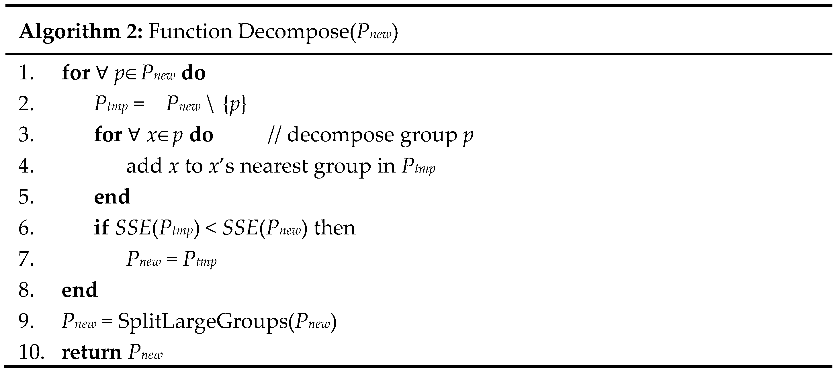
The proposed algorithm repeats two basic operations until both operations cannot yield a new and enhanced partition. The first operation, Decompose (line 4; Figure 1), fully decomposes each group to other groups if the resulting partition reduces the SSE (Figure 2). This operation is similar to the TFRP2 method described in Section 1. For each group p, this operation checks whether moving each record in p to its nearest group reduces the SSE of the solution.
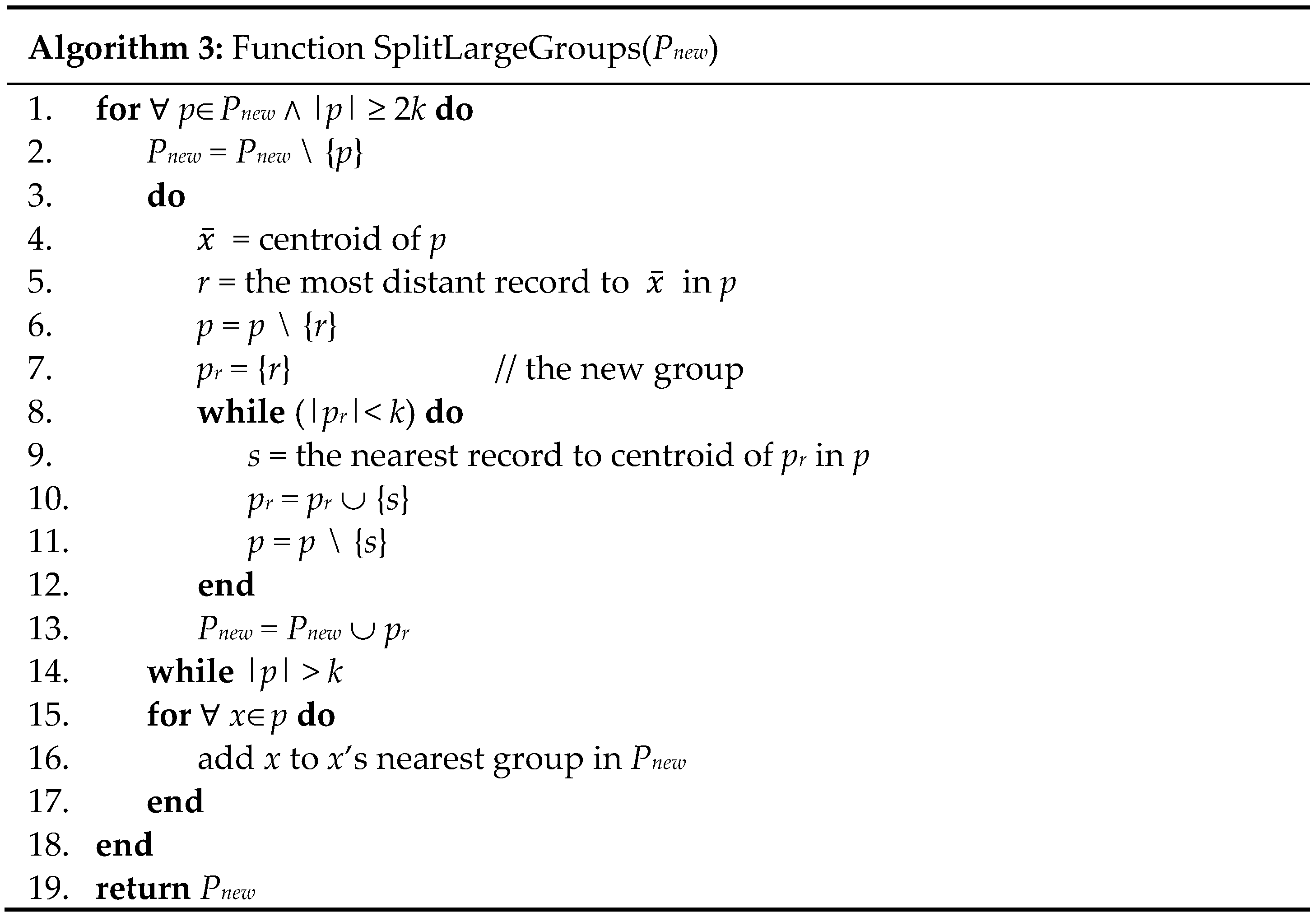
Because the Decompose operation could result in groups with 2k or more records, at its completion (line 9; Figure 2), this operation calls the SplitLargeGroups function to split any group with 2k or more records into several new groups such that the number of records in each new group is between k and 2k − 1. The SplitLargeGroups function (Figure 3) follows the CBFS method [7]. For any group p with 2k or more records, this function finds the record r∈p most distant from the centroid of p and forms a new group pr = {r} (lines 4–7; Figure 3). It then repeatedly adds to pr the record in p nearest to the centroid of pr until |pr| = k (lines 8–12; Figure 3). This process is repeated to generate new groups until |p| ≤ k (lines 3–14; Figure 3). The remaining records in p are added to their nearest groups (lines 15–17; Figure 3).
The second operation, Shrink (line 5; Figure 1), shrinks any group with more than k records (Figure 4). For any group p with more than k records, this operation searches for and moves the record xmin∈p such that moving xmin to another group reduces the SSE the most (lines 3–14; Figure 4). This process is repeated until p has only k records remaining or the resulting partition cannot further reduce the SSE (lines 2–15; Figure 4). Similar to the Decompose operation, the Shrink operation results in groups with 2k or more records and calls the SplitLargeGroups function to split these over-sized groups (line 17; Figure 4).
Notably, at most, groups are present in a solution. Because lines 1–8 in Figure 2 and lines 1–16 in Figure 4 require searching for the nearest group of each record, their time complexity is O (n2/k). The time complexity of the SplitLargeGroups function is O (k2 × n/k). Thus, an iteration of the Decompose and Shrink operations (lines 3–5; Figure 1) entails O (n2/k + k2 × n/k) = O (n2) time computation cost.
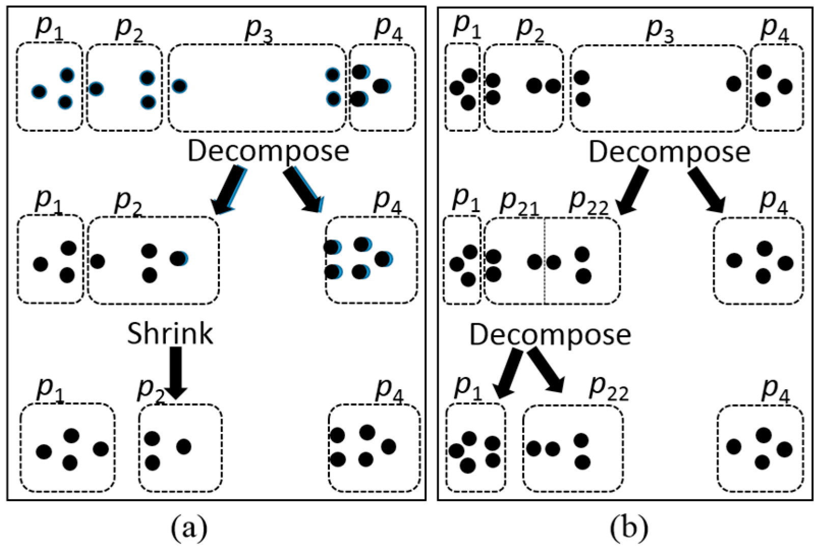
The proposed algorithm differs from previous work in two folds. First, the Shrink operation explores more opportunities for reducing SSE. Figure 5a gives an example. The upper part of Figure 5a shows the partition of 12 records (represented by small circles) generated by MDAV for k = 3. First, the Decompose operation decomposes group p3 and merges its content into groups p2 and p4, as shown in the middle part of Figure 5a. At this moment, the Decompose operation cannot further reduce the SSE of the partition result. However, the Shrink operation can reduce the SSE by moving a record from group p2 to group p1, as shown in the bottom part of Figure 5a.
Second, previous work performs the Decompose operation only once and ignores the fact that, after the Decompose operation, the grouping of records may have been changed and consequently new opportunities of reducing the SSE may appear [8,10,11]. Thus, the proposed algorithm repeatedly performs both Decompose and Shrink operations to explore such possibilities until it cannot improve the SSE any further. Figure 5b gives an example. The upper part of Figure 5b shows the partition of 13 records generated by MDAV for k = 3. At first, the Decompose operation can only reduce the SSE by decomposing group p3 and merging its content into groups p2 and p4. Because group p2 now has 2k or more records, it is split into two groups, p21 and p22, as shown in the middle part of Figure 5b. The emergence of the group p21 provides an opportunity to further reduce the SSE by decomposing group p21 and merging its content into groups p1 and p22, as shown in the bottom part of Figure 5b.
5. Experiment
5.1. Datasets
Three datasets commonly used for testing microaggregation performance were adopted in this experiment [9]: Tarragona (834 records in a 13-dimensional space), Census (1080 records in a 13-dimensional space), and EIA (4092 records with 11 numerical attributes). The original EIA dataset contained 15 attributes, out of which 13 were numeric. We discarded the two numeric attributes (YEAR and MONTH) and used the remaining 11 numeric attributes. Although there is no consensus on which attributes should be used, the aforementioned settings are the most widely adopted [7,8,9,11,13,14,29]. However, differences exist; for example, Ref. [15] used only 10 attributes from both the Census and EIA datasets. When comparing the experimental results from previous studies, one should check whether the same set of attributes was used in the experiments.
Consistent with most studies, before microaggregation, each attribute in each dataset is normalized to have zero mean and unit variance. This normalization step ensures that no single attribute has a disproportionate effect on the microagregation results. In Ref. [30], the theoretical bounds of information loss for these three datasets were derived. Without applying this normalization step, the information loss might be lower than the theoretical bound derived in Ref. [30] (e.g., Ref. [19]).
5.2. Experimental Settings
As described in Section 4, the proposed algorithm refines the solution generated using a fixed-size microaggregation approach. Seven fixed-size microaggregation approaches were adopted in this study: CBFS-NN, CBFS-NC, MDAV-NN, MDAV-NC, TFRP-NN, TFRP-NC and GSMS-NN. The prefix (i.e., CBFS, TFRP, MDAV, or GSMS, described in Section 3.1) indicates the heuristic used to select the first record of each group, and the suffix (i.e., NN or NC, described in Section 3.1) indicates the method used to grow the selected record to a group of k records. NN refers to forming a group using the selected record and its k − 1 nearest neighbors, and NC refers to forming a group by iteratively updating the centroid of the group and adding the record nearest to the centroid until the size of the group reaches k. MDAV-NN, CBFS-NC, TFRP-NN, and GSMS-NN are the same as MDAV [6], CBFS [7], TFRP [8], and GSMS [11] in the literature, respectively. Furthermore, we did not extend GSMS to GSMS-NC because maintaining the candidate groups in GSMS by using the NC method was too costly. Recalled from Section 3.1, the original GSMS [11] (referred to as GSMS-NN in this paper) needs to maintain a candidate group for each record which contains the record and its k-1 nearest unassigned neighbors. In each iteration, GSMS chooses one candidate group as a part of the final partition and updates the content of the other candidate groups to exclude those records in the selected candidate group. Because repeatedly updating the content of these candidate groups is time-consuming, GSMS maintains a priority queue for each record r that sorts all of the records by their distances to r. Thus, the original GSMS essentially uses the NN method to form each group. If GSMS adopts the NC method to form each group, then the priority queue technique is no longer feasible because the NC method is based on the distances to the groups’ centroids, not to a fixed record r as in the NN method. That is, each time a group’s centroid changes, the corresponding priority queue must be rebuilt, making GSMS-NC an inefficient alternative.
We applied the proposed algorithm to refine the solution generated by each of the seven fixed-size microaggregation approaches. The resulting methods are referred to as CBFS-NN3, CBFS-NC3, MDAV-NN3, MDAV-NC3, TFRP-NN3, TFRP-NC3, and GSMS-NN3. Moreover, as a performance baseline, we applied TFRP2 to refine the solution generated using each of the seven fixed-size microaggregation approaches. Specifically, TFRP2 was implemented by executing the Decompose function (Figure 2) once. We referred to the resulting methods as CBFS-NN2, CBFS-NC2, MDAV-NN2, MDAV-NC2, TFRP-NN2, TFRP-NC2, and GSMS-NN2. Notably, TFRP-NN2 and GSMS-NN2 are the same as TFRP2 [8] and GSMS-T2 [11], respectively, in the literature. Table 1 summarizes all of the tested methods.
5.3. Experimental Results
Table 2, Table 3 and Table 4 show the information loss using each method in Table 1 for different values of k in the Tarragona, Census, and EIA datasets, respectively. For brevity, we refer to those methods without applying any refinement heuristic as the Unrefined methods (i.e., all method names without a suffix “2” or “3” in the first column of Table 1), and those methods applying the TFRP2 heuristic to refine a solution as the TFRP2 methods (i.e., all method names with a suffix “2”). Although the TFRP2 methods always achieved a lower information loss than their corresponding Unrefined methods did on the Census and EIA datasets, our methods (i.e., all method names with a suffix “3”) could yield an even lower information loss than the TFRP2 methods did on these two datasets (Table 3 and Table 4).
The italicized entries in Table 2 indicate that, for the Tarragona dataset, the TFRP2 methods could not improve the solutions provided by the Unrefined methods only in five cases (i.e., CBFS-NN, CBFS-NC and GSMS-NN at k = 3, and MDAV-NN at k = 5 and 10). However, our methods could not improve the Unrefined methods only in three cases (i.e., CBFS-NN, CBFS-NC and GSMS-NN at k = 3). Therefore, our methods are more effective than the TFRP2 methods in refining the solutions of the Unrefined methods. The best result for each k value is shown in bold in Table 2, Table 3 and Table 4.
In Table 5, our best results from Table 2, Table 3 and Table 4 are compared with the best results of the almost quadratic time microaggregation algorithms from [11]. In all cases, less information loss was observed using our methods. Furthermore, for the Census dataset with k = 10 and for the EIA dataset with k = 5 or 10, the best solutions obtained by our methods in Table 5 are the most superior in the literature [11,13].
Table 6 indicates the cases in which our methods yielded a lower information loss than those in [11]. Among the seven methods, both CBFS-NC3 and GSMS-NN3 outperformed the results from [11] for six of the nine cases. Table 5 confirms that CBFS-NC3 and GSMS-NN3 also yielded the best results for two and three of the nine cases, respectively.
6. Conclusions
In this paper, we proposed an algorithm to effectively refine the solution generated using a fixed-size microaggregation approach. Although the fixed-size approaches (i.e., methods without a suffix “2” or “3”) do not always generate an ideal solution, the experimental results in Table 2, Table 3 and Table 4 concluded that the refinement methods (i.e., methods with a suffix “2” or “3”) help with improving the information loss of the results of the fixed-size approaches. Moreover, our proposed refinement methods (i.e., methods with a suffix “3”) can further reduce the information loss of the TFRP2 refinement methods (i.e., methods with a suffix “2”) and yield an information loss lower than those reported in the literature [11].
The TFRP2 refinement heuristic checks each group for the opportunity of reducing the information loss via decomposing the group. Our proposed algorithm (Figure 1) can discover more opportunities such as this than the TFRP2 refinement heuristic does because the proposed algorithm can not only decompose but also shrink a group. Moreover, the TFRP2 refinement heuristic checks each group only once, but our proposed algorithm checks each group more than once. Because one refinement step could result in another refinement step that did not exist initially, our proposed algorithm is more effective in reducing the information loss than the TFRP2 refinement heuristic does.
The proposed algorithm is essentially a local search method within the feasible domain of the solution space. In other words, we refined a solution while enforcing the k-anonymity constraint (i.e., each group in a solution contains no fewer than k records). However, the local search method could still be trapped in the local optima. A possible solution is to allow the local search method to temporarily step out of the feasible domain. Another possible solution is to allow the information loss to increase within a local search step but at a low probability, similar to the simulated annealing algorithms. The extension of the local search method warrants further research.
Author Contributions
Conceptualization, L.K. and J.-L.L.; Data curation, Z.-Q.P.; Funding acquisition, J.-L.L.; Methodology, J.-L.L.; Software, L.K.; Supervision, J.-L.L.; Validation, L.K.; Visualization, A.S.S.; Writing—Original draft, J.-L.L.; Writing—Review and editing, L.K. Overall contribution: L.K. (50%), J.-L.L. (40%), Z.-Q.P. (5%), and A.S.S. (5%).
Funding
This research is supported by the Ministry of Science and Technology (MOST), Taiwan, under Grant MOST 106-2221-E-155-038.
Conflicts of Interest
The authors declare no conflict of interest.
References
- Domingo-Ferrer, J.; Torra, V. Privacy in data mining. Data Min. Knowl. Discov. 2005, 11, 117–119. [Google Scholar] [CrossRef]
- Willenborg, L.; Waal, T.D. Data Analytic Impact of SDC Techniques on Microdata. In Elements of Statistical Disclosure Control; Springer: New York, NY, USA, 2000. [Google Scholar]
- Sweeney, L. k-anonymity: A model for protecting privacy. Int. J. Uncertain. Fuzziness Knowl. Based Syst. 2002, 10, 557–570. [Google Scholar] [CrossRef]
- Hansen, S.L.; Mukherjee, S. A polynomial algorithm for optimal univariate microaggregation. IEEE Trans. Knowl. Data Eng. 2003, 15, 1043–1044. [Google Scholar] [CrossRef] [Green Version]
- Oganian, A.; Domingo-Ferrer, J. On the complexity of optimal microaggregation for statistical disclosure control. Stat. J. U. N. Econ. Comm. Eur. 2001, 18, 345–353. [Google Scholar]
- Domingo-Ferrer, J.; Torra, V. Ordinal, continuous and heterogeneous k-anonymity through microaggregation. Data Min. Knowl. Discov. 2005, 11, 195–212. [Google Scholar] [CrossRef]
- Laszlo, M.; Mukherjee, S. Minimum spanning tree partitioning algorithm for microaggregation. IEEE Trans. Knowl. Data Eng. 2005, 17, 902–911. [Google Scholar] [CrossRef] [Green Version]
- Chang, C.C.; Li, Y.C.; Huang, W.H. TFRP: An efficient microaggregation algorithm for statistical disclosure control. J. Syst. Softw. 2007, 80, 1866–1878. [Google Scholar] [CrossRef]
- Domingo-Ferrer, J.; Martinez-Balleste, A.; Mateo-Sanz, J.M.; Sebe, F. Efficient multivariate data-oriented microaggregation. Int. J. Large Data Bases 2006, 15, 355–369. [Google Scholar] [CrossRef]
- Lin, J.L.; Wen, T.H.; Hsieh, J.C.; Chang, P.C. Density-based microaggregation for statistical disclosure control. Expert Syst. Appl. 2010, 37, 3256–3263. [Google Scholar] [CrossRef]
- Panagiotakis, C.; Tziritas, G. Successive group selection for microaggregation. IEEE Trans. Knowl. Data Eng. 2013, 25, 1191–1195. [Google Scholar] [CrossRef]
- Mortazavi, R.; Jalili, S. Fast data-oriented microaggregation algorithm for large numerical datasets. Knowl. Based Syst. 2014, 67, 195–205. [Google Scholar] [CrossRef]
- Aloise, D.; Araújo, A. A derivative-free algorithm for refining numerical microaggregation solutions. Int. Trans. Oper. Res. 2015, 22, 693–712. [Google Scholar] [CrossRef]
- Mortazavi, R.; Jalili, S.; Gohargazi, H. Multivariate microaggregation by iterative optimization. Appl. Intell. 2013, 39, 529–544. [Google Scholar] [CrossRef]
- Laszlo, M.; Mukherjee, S. Iterated local search for microaggregation. J. Syst. Softw. 2015, 100, 15–26. [Google Scholar] [CrossRef]
- Mortazavi, R.; Jalili, S. A novel local search method for microaggregation. ISC Int. J. Inf. Secur. 2015, 7, 15–26. [Google Scholar]
- Domingo-Ferrer, J.; Mateo-Sanz, J.M. Practical data-oriented microaggregation for statistical disclosure control. IEEE Trans. Knowl. Data Eng. 2002, 14, 189–201. [Google Scholar] [CrossRef]
- Kabir, M.E.; Mahmood, A.N.; Wang, H.; Mustafa, A. Microaggregation sorting framework for K-anonymity statistical disclosure control in cloud computing. IEEE Trans. Cloud Comput. 2015. Available online: http://doi.ieeecomputersociety.org/10.1109/TCC.2015.2469649 (accessed on 1 June 2018). [CrossRef]
- Kabir, M.E.; Wang, H.; Zhang, Y. A pairwise-systematic microaggregation for statistical disclosure control. In Proceedings of the IEEE 10th International Conference on Data Mining (ICDM), Sydney, NSW, Australia, 13–17 December 2010; pp. 266–273. [Google Scholar]
- Kabir, M.E.; Wang, H. Systematic clustering-based microaggregation for statistical disclosure control. In Proceedings of the 2010 Fourth International Conference on Network and System Security, Melbourne, VIC, Australia, 1–3 September 2010; pp. 435–441. [Google Scholar]
- Sun, X.; Wang, H.; Li, J.; Zhang, Y. An approximate microaggregation approach for microdata protection. Expert Syst. Appl. 2012, 39, 2211–2219. [Google Scholar] [CrossRef] [Green Version]
- Panagiotakis, C.; Tziritas, G. A minimum spanning tree equipartition algorithm for microaggregation. J. Appl. Stat. 2015, 42, 846–865. [Google Scholar] [CrossRef]
- Zahn, C.T. Graph-theoretical methods for detecting and describing gestalt clusters. IEEE Trans. Comput. 1971, C-20, 68–86. [Google Scholar] [CrossRef]
- Ward, J.H. Hierarchical grouping to optimize an objective function. J. Am. Stat. Assoc. 1963, 58, 236–244. [Google Scholar] [CrossRef]
- Machanavajjhala, A.; Kifer, D.; Gehrke, J.; Venkitasubramaniam, M. l-diversity: Privacy beyond k-anonymity. ACM Trans. Knowl. Discov. Data 2007, 1, 3. [Google Scholar] [CrossRef]
- Li, N.; Li, T.; Venkatasubramanian, S. t-closeness: Privacy beyond k-anonymity and l-diversity. In Proceedings of the 2007 IEEE 23rd International Conference on Data Engineering, Istanbul, Turkey, 15–20 April 2007; pp. 106–115. [Google Scholar]
- Sun, X.; Wang, H.; Li, J.; Zhang, Y. Satisfying privacy requirements before data anonymization. Comput. J. 2012, 55, 422–437. [Google Scholar] [CrossRef]
- Domingo-Ferrer, J.; Soria-Comas, J. Steered microaggregation: A unified primitive for anonymization of data sets and data streams. In Proceedings of the 2017 IEEE International Conference on Data Mining Workshops (ICDMW), New Orleans, LA, USA, 18–21 November 2017; pp. 995–1002. [Google Scholar]
- Domingo-Ferrer, J.; Sebe, F.; Solanas, A. A polynomial-time approximation to optimal multivariate microaggregation. Comput. Math. Appl. 2008, 55, 714–732. [Google Scholar] [CrossRef]
- Aloise, D.; Hansen, P.; Rocha, C.; Santi, É. Column generation bounds for numerical microaggregation. J. Glob. Optim. 2014, 60, 165–182. [Google Scholar] [CrossRef]
Figure 1.
Proposed algorithm.

Figure 2.
Decompose function.

Figure 3.
SplitLargeGroups function.

Figure 4.
Shrink function.
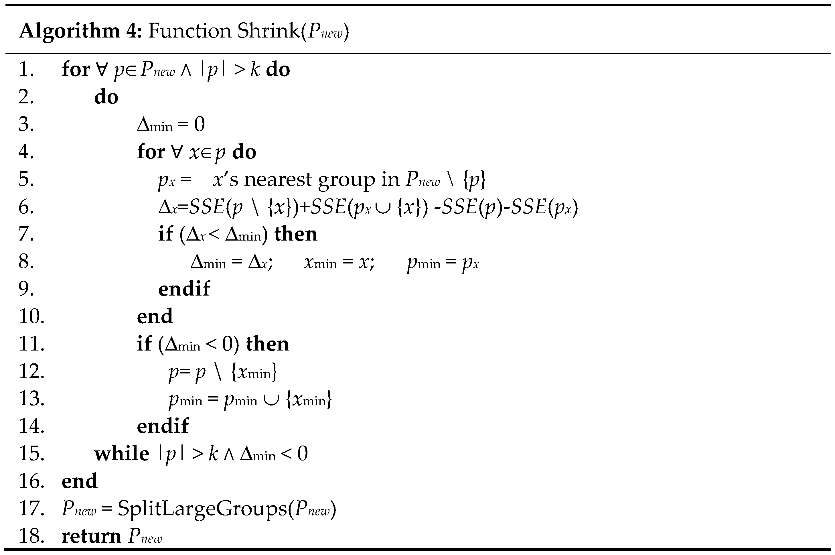
Figure 5.
Two examples. (a) A Shrink operation after a Decompose operation reduces the information loss; (b) A Decompose operation after another Decompose operation reduces the information loss.
Figure 5.
Two examples. (a) A Shrink operation after a Decompose operation reduces the information loss; (b) A Decompose operation after another Decompose operation reduces the information loss.


Table 1.
Tested methods.
| Tested Method | Heuristic for Selecting the 1st Record of Each Group | Heuristic for Growing a Group to Size k | Method for Refining a Solution |
|---|---|---|---|
| CBFS-NN | CBFS | Nearest Neighbors to 1st record | None |
| CBFS-NN2 | CBFS | Nearest Neighbors to 1st record | TFRP2 |
| CBFS-NN3 | CBFS | Nearest Neighbors to 1st record | Our method in Figure 1 |
| CBFS-NC | CBFS | Nearest to group’s Centroid | None |
| CBFS-NC2 | CBFS | Nearest to group’s Centroid | TFRP2 |
| CBFS-NC3 | CBFS | Nearest to group’s Centroid | Our method in Figure 1 |
| MDAV-NN | MDAV | Nearest Neighbors to 1st record | None |
| MDAV-NN2 | MDAV | Nearest Neighbors to 1st record | TFRP2 |
| MDAV-NN3 | MDAV | Nearest Neighbors to 1st record | Our method in Figure 1 |
| MDAV-NC | MDAV | Nearest to group’s Centroid | None |
| MDAV-NC2 | MDAV | Nearest to group’s Centroid | TFRP2 |
| MDAV-NC3 | MDAV | Nearest to group’s Centroid | Our method in Figure 1 |
| TFRP-NN | TFRP | Nearest Neighbors to 1st record | None |
| TFRP-NN2 | TFRP | Nearest Neighbors to 1st record | TFRP2 |
| TFRP-NN3 | TFRP | Nearest Neighbors to 1st record | Our method in Figure 1 |
| TFRP-NC | TFRP | Nearest to group’s Centroid | None |
| TFRP-NC2 | TFRP | Nearest to group’s Centroid | TFRP2 |
| TFRP-NC3 | TFRP | Nearest to group’s Centroid | Our method in Figure 1 |
| GSMS-NN | GSMS | Nearest Neighbors to 1st record | None |
| GSMS-NN2 | GSMS | Nearest Neighbors to 1st record | TFRP2 |
| GSMS-NN3 | GSMS | Nearest Neighbors to 1st record | Our method in Figure 1 |
Table 2.
The information loss (%) in the Tarragona dataset.
| Method/k | 3 | 4 | 5 | 10 | 20 | 30 |
|---|---|---|---|---|---|---|
| CBFS-NN | 16.966 | 19.730 | 22.819 | 33.215 | 42.955 | 49.489 |
| CBFS-NN2 | 16.966 | 19.227 | 22.588 | 33.211 | 42.944 | 49.481 |
| CBFS-NN3 | 16.966 | 18.651 | 22.268 | 33.173 | 42.872 | 49.404 |
| CBFS-NC | 15.617 | 19.230 | 22.609 | 37.105 | 47.685 | 56.042 |
| CBFS-NC2 | 15.617 | 19.210 | 22.150 | 36.892 | 46.415 | 53.212 |
| CBFS-NC3 | 15.617 | 19.172 | 21.434 | 36.290 | 41.848 | 47.231 |
| MDAV-NN | 16.9326 | 19.546 | 22.4613 | 33.192 | 43.195 | 49.483 |
| MDAV-NN2 | 16.9324 | 19.029 | 22.4613 | 33.192 | 43.099 | 49.460 |
| MDAV-NN3 | 16.9320 | 18.434 | 22.4612 | 33.184 | 42.771 | 49.261 |
| MDAV-NC | 15.631 | 19.176 | 22.712 | 36.992 | 47.705 | 56.370 |
| MDAV-NC2 | 15.617 | 19.140 | 22.284 | 36.955 | 46.167 | 52.705 |
| MDAV-NC3 | 15.598 | 19.068 | 21.409 | 36.389 | 41.122 | 47.297 |
| TFRP-NN | 17.112 | 19.995 | 23.412 | 33.557 | 43.416 | 50.187 |
| TFRP-NN2 | 17.070 | 19.715 | 23.136 | 33.405 | 43.343 | 49.965 |
| TFRP-NN3 | 16.954 | 19.275 | 22.408 | 32.866 | 42.652 | 48.512 |
| TFRP-NC | 17.629 | 19.511 | 23.222 | 35.645 | 47.654 | 55.604 |
| TFRP-NC2 | 16.702 | 19.374 | 23.171 | 35.400 | 46.317 | 53.050 |
| TFRP-NC3 | 16.021 | 19.233 | 22.839 | 34.909 | 41.358 | 47.034 |
| GSMS-NN | 16.610 | 19.050 | 21.948 | 33.234 | 43.023 | 49.433 |
| GSMS-NN2 | 16.610 | 19.046 | 21.723 | 33.230 | 43.008 | 49.429 |
| GSMS-NN3 | 16.610 | 19.039 | 21.311 | 33.208 | 42.932 | 49.395 |
Table 3.
The information loss (%) in the Census dataset.
| Method/k | 3 | 4 | 5 | 10 | 20 | 30 |
|---|---|---|---|---|---|---|
| CBFS-NN | 5.654 | 7.441 | 8.884 | 14.001 | 19.469 | 23.881 |
| CBFS-NN2 | 5.648 | 7.439 | 8.848 | 13.902 | 19.384 | 23.651 |
| CBFS-NN3 | 5.644 | 7.406 | 8.554 | 12.809 | 17.938 | 21.509 |
| CBFS-NC | 5.348 | 7.173 | 8.685 | 14.341 | 21.390 | 26.505 |
| CBFS-NC2 | 5.337 | 7.165 | 8.656 | 14.117 | 20.470 | 24.848 |
| CBFS-NC3 | 5.325 | 7.139 | 8.575 | 12.672 | 17.365 | 20.326 |
| MDAV-NN | 5.692 | 7.495 | 9.088 | 14.156 | 19.578 | 23.407 |
| MDAV-NN2 | 5.683 | 7.434 | 9.054 | 14.017 | 19.492 | 23.289 |
| MDAV-NN3 | 5.660 | 7.218 | 8.950 | 12.809 | 18.129 | 21.201 |
| MDAV-NC | 5.343 | 7.290 | 8.945 | 14.361 | 21.364 | 25.123 |
| MDAV-NC2 | 5.335 | 7.265 | 8.898 | 14.043 | 20.091 | 23.686 |
| MDAV-NC3 | 5.334 | 7.222 | 8.698 | 12.648 | 17.481 | 20.647 |
| TFRP-NN | 5.864 | 7.965 | 9.252 | 14.369 | 20.167 | 23.607 |
| TFRP-NN2 | 5.805 | 7.831 | 9.039 | 14.042 | 19.817 | 23.063 |
| TFRP-NN3 | 5.735 | 7.428 | 8.408 | 13.024 | 18.211 | 21.112 |
| TFRP-NC | 5.645 | 7.636 | 9.301 | 14.834 | 21.719 | 26.725 |
| TFRP-NC2 | 5.546 | 7.496 | 9.037 | 14.265 | 20.555 | 25.031 |
| TFRP-NC3 | 5.466 | 7.382 | 8.796 | 12.963 | 17.973 | 20.892 |
| GSMS-NN | 5.564 | 7.254 | 8.686 | 13.549 | 18.792 | 22.432 |
| GSMS-NN2 | 5.545 | 7.251 | 8.597 | 13.452 | 18.451 | 22.354 |
| GSMS-NN3 | 5.535 | 7.240 | 8.367 | 13.085 | 17.230 | 21.089 |
Table 4.
The information loss (%) in the EIA dataset.
| Method/k | 3 | 4 | 5 | 10 | 20 | 30 |
|---|---|---|---|---|---|---|
| CBFS-NN | 0.478 | 0.671 | 1.740 | 3.512 | 7.053 | 10.919 |
| CBFS-NN2 | 0.416 | 0.614 | 0.960 | 2.644 | 6.981 | 10.854 |
| CBFS-NN3 | 0.402 | 0.587 | 0.803 | 2.036 | 6.823 | 10.605 |
| CBFS-NC | 0.470 | 0.672 | 1.533 | 3.276 | 7.628 | 10.084 |
| CBFS-NC2 | 0.426 | 0.612 | 0.891 | 2.552 | 7.410 | 10.046 |
| CBFS-NC3 | 0.415 | 0.574 | 0.762 | 2.282 | 7.110 | 10.038 |
| MDAV-NN | 0.483 | 0.671 | 1.667 | 3.840 | 7.095 | 10.273 |
| MDAV-NN2 | 0.417 | 0.614 | 0.969 | 2.931 | 7.010 | 10.192 |
| MDAV-NN3 | 0.401 | 0.587 | 0.802 | 2.022 | 6.806 | 9.873 |
| MDAV-NC | 0.471 | 0.677 | 1.459 | 3.058 | 7.641 | 9.984 |
| MDAV-NC2 | 0.428 | 0.612 | 0.962 | 2.744 | 7.427 | 9.946 |
| MDAV-NC3 | 0.415 | 0.573 | 0.795 | 2.298 | 7.109 | 9.937 |
| TFRP-NN | 0.513 | 0.680 | 1.768 | 3.543 | 7.087 | 11.116 |
| TFRP-NN2 | 0.419 | 0.613 | 0.969 | 2.669 | 6.977 | 10.993 |
| TFRP-NN3 | 0.405 | 0.585 | 0.8 | 2.04 | 6.771 | 10.491 |
| TFRP-NC | 0.465 | 0.674 | 1.670 | 3.288 | 7.663 | 11.286 |
| TFRP-NC2 | 0.420 | 0.607 | 0.887 | 2.545 | 7.443 | 10.684 |
| TFRP-NC3 | 0.410 | 0.574 | 0.779 | 2.289 | 7.116 | 10.324 |
| GSMS-NN | 0.469 | 0.669 | 1.713 | 3.313 | 6.958 | 11.384 |
| GSMS-NN2 | 0.407 | 0.610 | 0.890 | 2.569 | 6.859 | 10.704 |
| GSMS-NN3 | 0.394 | 0.59 | 0.796 | 2.101 | 6.647 | 9.314 |
Table 5.
Best information loss (IL) from Ref. [11] and from our methods.
Table 5.
Best information loss (IL) from Ref. [11] and from our methods.
| Dataset | k | Best from [11] | Our Best | ||
|---|---|---|---|---|---|
| IL*100 | Method | IL*100 | Method | ||
| Tarragona | 3 | 16.36 | GSMS-T2 | 15.598 | MDAV-NC3 |
| Tarragona | 5 | 21.72 | GSMS-T2 | 21.311 | GSMS-NC3 |
| Tarragona | 10 | 33.18 | MD-MHM | 32.866 | TFRP-NN3 |
| Census | 3 | 5.53 | GSMS-T2 | 5.325 | CBFS-NC3 |
| Census | 5 | 8.58 | GSMS-T2 | 8.367 | GSMS-NN3 |
| Census | 10 | 13.42 | GSMS-T2 | 12.648 | MDAV-NC3 |
| EIA | 3 | 0.401 | GSMS-T2 | 0.394 | GSMS-NN3 |
| EIA | 5 | 0.87 | GSMS-T2 | 0.762 | CBFS-NC3 |
| EIA | 10 | 2.17 | μ-Approx | 2.022 | MDAV-NN3 |
Table 6.
The cases that our methods yield lower information loss than the best results from Ref. [11].
Table 6.
The cases that our methods yield lower information loss than the best results from Ref. [11].
| Method | Tarragona | Census | EIA | ||||||
|---|---|---|---|---|---|---|---|---|---|
| k = 3 | k = 5 | k = 10 | k = 3 | k = 5 | k = 10 | k = 3 | k = 5 | k = 10 | |
| CBFS-NN3 | V | V | V | V | V | ||||
| CBFS-NC3 | V | V | V | V | V | V | |||
| MDAV-NN3 | V | V | V | ||||||
| MDAV-NC3 | V | V | V | V | V | ||||
| TFRP-NN3 | V | V | V | V | V | ||||
| TFRP-NC3 | V | V | V | V | |||||
| GSMS-NN3 | V | V | V | V | V | V | |||
© 2018 by the authors. Licensee MDPI, Basel, Switzerland. This article is an open access article distributed under the terms and conditions of the Creative Commons Attribution (CC BY) license (http://creativecommons.org/licenses/by/4.0/).
Share and Cite
MDPI and ACS Style
Khomnotai, L.; Lin, J.-L.; Peng, Z.-Q.; Santra, A.S. Iterative Group Decomposition for Refining Microaggregation Solutions. Symmetry 2018, 10, 262. https://doi.org/10.3390/sym10070262
AMA Style
Khomnotai L, Lin J-L, Peng Z-Q, Santra AS. Iterative Group Decomposition for Refining Microaggregation Solutions. Symmetry. 2018; 10(7):262. https://doi.org/10.3390/sym10070262
Chicago/Turabian StyleKhomnotai, Laksamee, Jun-Lin Lin, Zhi-Qiang Peng, and Arpita Samanta Santra. 2018. "Iterative Group Decomposition for Refining Microaggregation Solutions" Symmetry 10, no. 7: 262. https://doi.org/10.3390/sym10070262
Note that from the first issue of 2016, this journal uses article numbers instead of page numbers. See further details here.