3.1. Bi-Mode Embedding
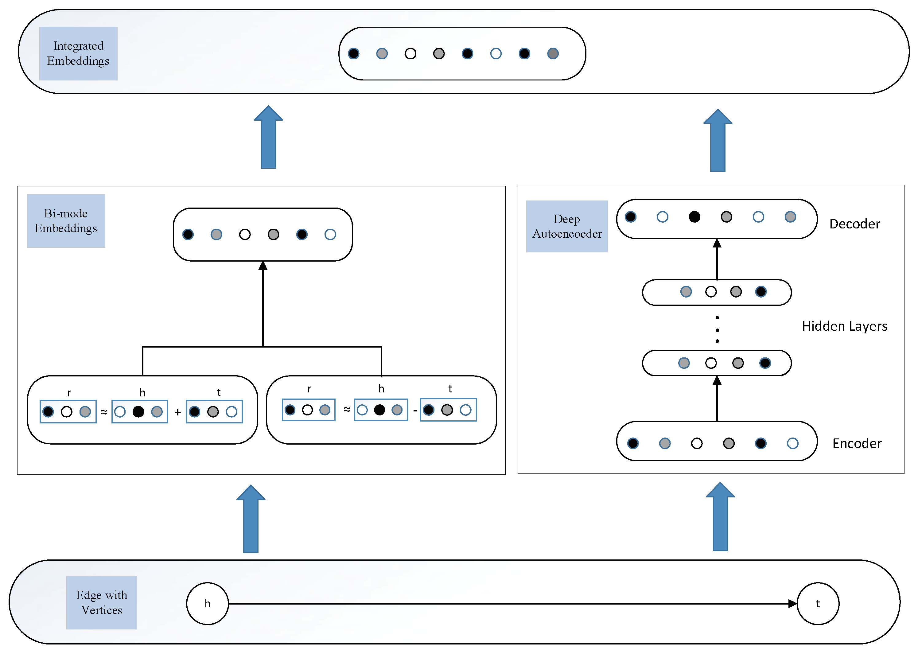
Inspired by knowledge representation, which can extract relation features efficiently, we borrow concepts such as triplets in KG to help realize the bi-mode embedding. We will firstly introduce the common notations. A triplet is denoted as , where h denotes a head entity, r denotes a relation, and t denotes a tail entity, where head entities and tail entities are actually vertices in a network, and relations are actually edges. The bold letter , , represent the embeddings of . To discriminate the add-mode and subtract-mode, we denote their embeddings as , , and , , , respectively. The entity and relations take values in , where n is the dimension of entity and relation embeddings spaces. Next, we will introduce the detailed mechanism of add-mode and subtract-mode.
Add-Mode Embedding: The basic idea of add-mode embedding is that a relation is the abstraction of all the features of entity pairs. That is, some most common features will burst and individual features will correspondingly fade by consolidating all the features of entity pairs.
For each triplet , a head entity h and a tail entity t constitute an entity pair together, denoted as . Given an entity pair , there could be plenty of relations fitting the pair; on the other hand, one relation could also match a large number of entity pairs. Therefore, if we incorporate all the shared features of these entity pairs, this could be used to represent the unique features possessed by relation r, which is unlikely represented by other entity pairs without having relation r. That is, , mathematically.
Motivated by the above theory, we propose an add-mode embedding model that demonstrates that all the shared features of head entities and tail entities should be close to the features of relation
r. In other words, when a triplet
exists, it is expected that
From this,
should be the closest relation of
; otherwise
should be far away from
. Moreover, under an energy-based framework, the energy of a triplet is equal to the distance between
and
, which could be measured by either
or
norms. Thus, the objective function can be represented as follows:
Subtract-Mode Embedding: Add-mode embedding can express the entity-shared features of relations, but neglects the entity-specific features. Recall the example that Trump is the president of America, and Putin is the president of Russia. Add-mode embedding could easily capture the representation features between Trump (resp. Putin) and America (resp. Russia). Nevertheless, if we intentionally pair Trump with Russia, add-mode embedding may falsely figure that the corrupted entity pair as correct, as the shared features between Trump and Russia may be fairly close to the features of relation Presidentof. We attribute this to the fact that add-mode embedding only focuses on shared features while it underestimates the significance of the individual features of entities.
To cover the shortage of add-mode embedding, we further adopt the subtract-mode embedding so as to capture the entity-specific features. For a triplet
, the embedding
of relation
r describes the discrepancies between
h and
t by calculating the differences between their embeddings. That is,
, mathematically. In this case, it is expected that
is close to
, meanwhile it is far away from other entities. Similarly, the objective function can be represented as follows:
Consequently, we can obtain the overall objective function of bi-mode embedding via integrating the two complementary methods together:
To learn such embeddings, for each triplet
and its corrupted sample
, we minimize the following margin-based ranking loss function over the training set,
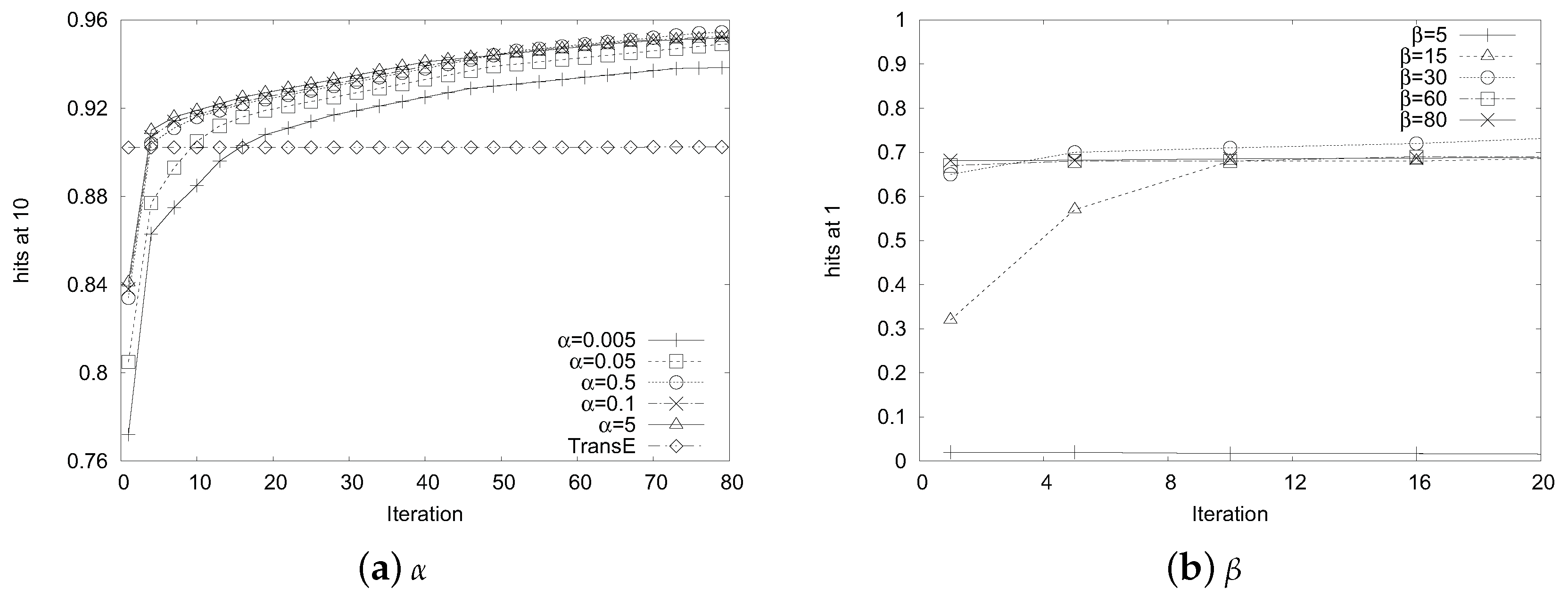
where
is a margin hyperparameter and the loss function above encourages the discrimination between positive triplets and corrupted triplets.
is a negative sample that is obtained by randomly replacing the original head or tail entity (resp. relation) with another disconnected entity (resp. relation).
3.2. Deep Autoencoder
Here, we introduce the detailed mechanism of a deep autoencoder to illustrate its ability to capture the structural information of edges. Firstly, for ease of understanding, we propose a bold concept in that we regard edges as nodes and vertices as links to build a new network. However, such changes will not influence the overall structure of the original network, so we see this concept as quite acceptable.
Given a modified network
, where
N denotes the nodes that are actually edges and
L denotes the links that are actually vertices, we can obtain its adjacency matrix
of nodes.
S contains
m instances denoted as
. For each instance
,
if and only if node
and node
have a connected link. Hence,
expresses the neighborhood structure of the node
and
S encodes the neighborhood structure of each node, thus obtaining the global structure of the network. Next, we introduce how we incorporate the adjacency matrix
into the traditional deep autoencoder [
7].
The deep autoencoder comprises two parts—i.e., the encoder part and the decoder part. The encoder consists of multiple nonlinear functions mapping the input data to the representation space. The decoder also consists of multiple nonlinear functions that map the representations from representation space to reconstruction space. Given the input
, the hidden representations for each layer are presented as follows:
denotes the activation function and we apply the
sigmoid function in this paper. After obtaining
, we can correspondingly obtain the output
by reversing the calculation process of the encoder. The autoencoder aims to minimize the reconstruction error of the output and the input. The loss function is shown as follows:
Authors in [
7] proved that although minimizing the reconstruction loss does not explicitly preserve the similarity between samples, its reconstruction criterion can smoothly capture the data manifolds, thus preserving the similarity between samples. Therefore, considering our case wherein we use the adjacency matrix
as the input to the autoencoder (i.e.,
), since
encodes the neighborhood structure of node
, the reconstruction calculation will make the nodes that have similar neighborhood structure have similar representations as well.
However, we cannot directly apply this reconstruction function to our problem due to the sparsity of the input matrix. That is, the number of zero elements in
is much larger than that of non-zero elements, which means that the autoencoder tends to reconstruct the zero elements instead of non-zero ones. This is not what we expect. Hence, we impose more penalty to the reconstruction error of the non-zero element than that of zero elements. The modified objective function is shown as follows:
where ⊙ denotes the Hadamard dot, i.e., element-wise multiplication,
. If
,
; otherwise,
, where
is the hyperparameter to balance the weight of non-zero elements in autoencoder. Now, by utilizing the modified deep autoencoder with the input adjacency matrix
, the nodes that have similar structures will be mapped closely in the representation space, which is guaranteed by the reconstruction criterion. Namely, a deep autoencoder could capture the structural information of the network by the reconstructing process on nodes (in our case, edges).


