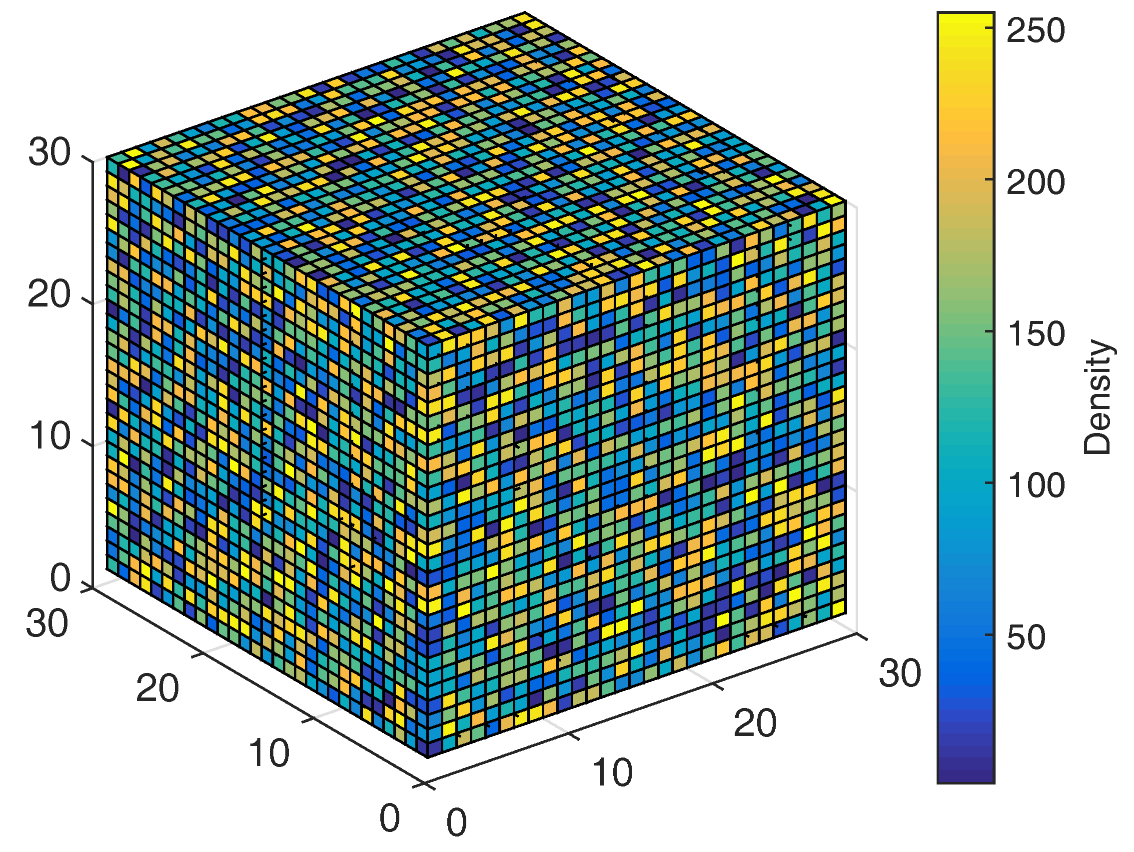
Figure 1.
The uniform noise in the color scale plot shows the irregular density of water droplets in a cloud hypertexture. In the MATLAB four dimensional plot, it is possible to observe the nature of atmospheric vapour in the color values in the cube.
Figure 1.
The uniform noise in the color scale plot shows the irregular density of water droplets in a cloud hypertexture. In the MATLAB four dimensional plot, it is possible to observe the nature of atmospheric vapour in the color values in the cube.
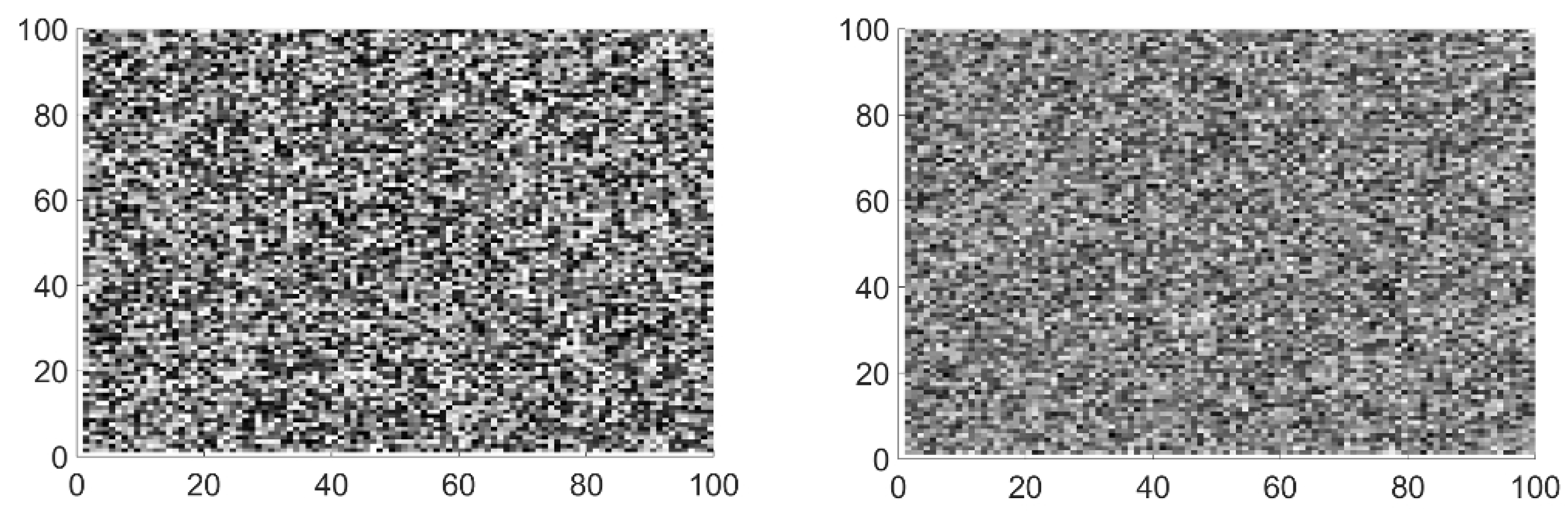
Figure 2.
Bi-dimensional representation of uniform noise (left) and fractal Brownian motion (fBm) noise (right). The base noise on the left is sharper while the fBm is softer due to the octave accumulation.
Figure 2.
Bi-dimensional representation of uniform noise (left) and fractal Brownian motion (fBm) noise (right). The base noise on the left is sharper while the fBm is softer due to the octave accumulation.
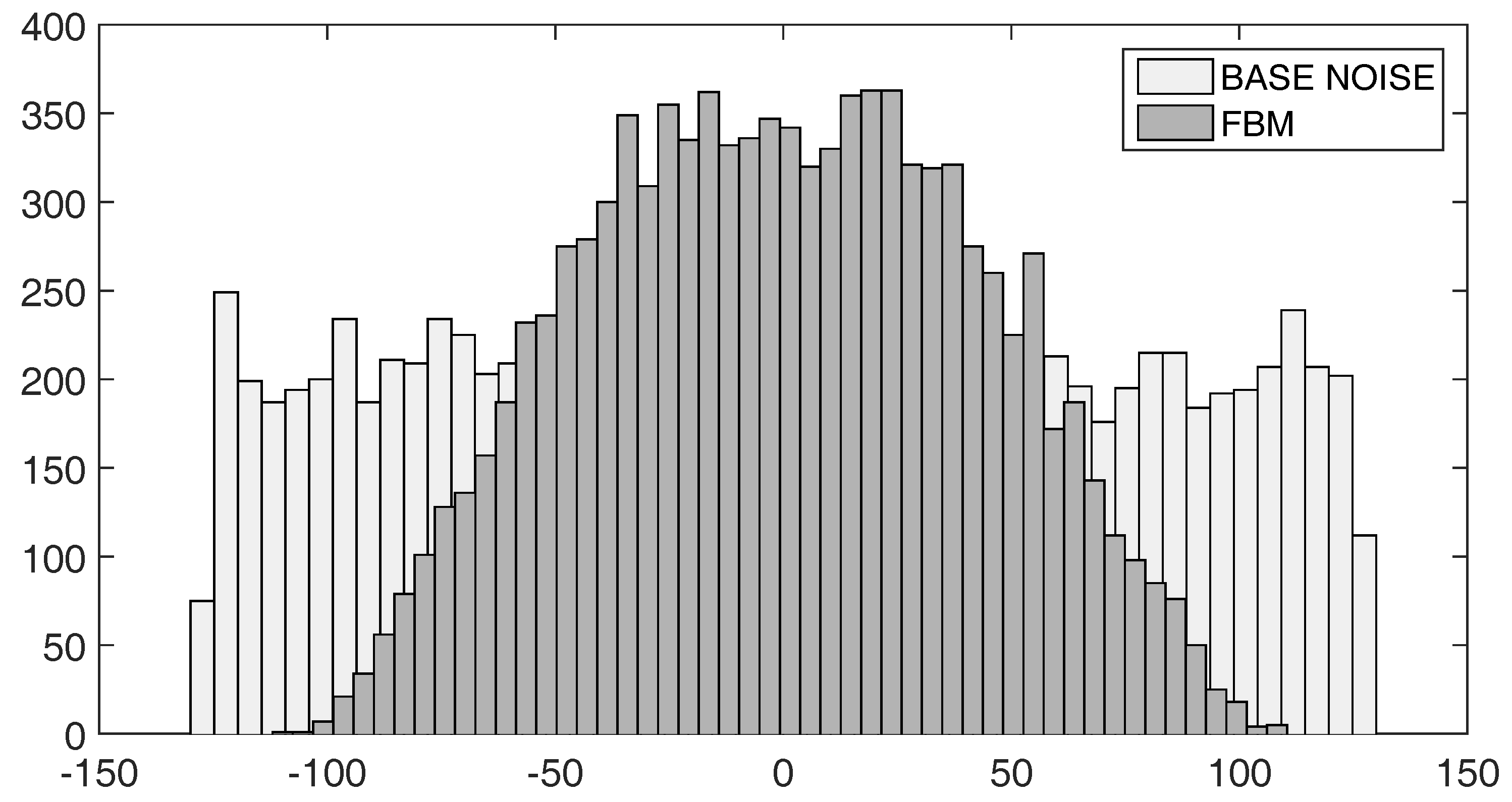
Figure 3.
Histogram of uniform noise (light gray) and fBm noise (dark gray). The fBm noise has a Gaussian-like distribution.
Figure 3.
Histogram of uniform noise (light gray) and fBm noise (dark gray). The fBm noise has a Gaussian-like distribution.
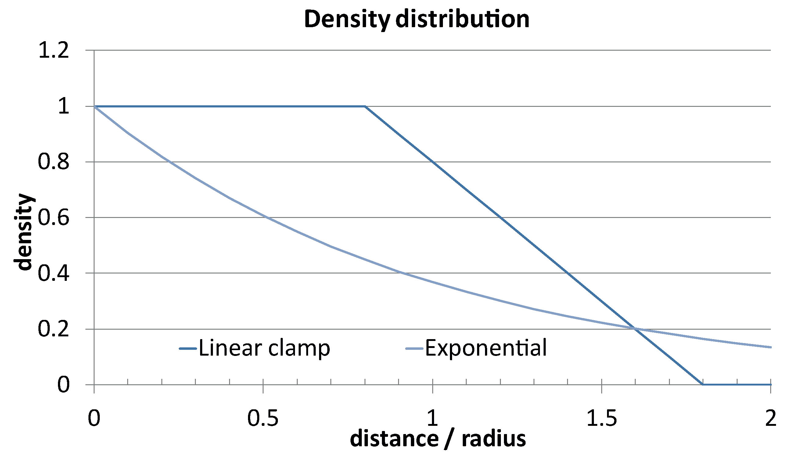
Figure 4.
Distance/density relationship. The greater the distance between the ray and the sphere center, the lower the density of water vapour. The exponential approach gives natural realism by softening the cloud borders.
Figure 4.
Distance/density relationship. The greater the distance between the ray and the sphere center, the lower the density of water vapour. The exponential approach gives natural realism by softening the cloud borders.
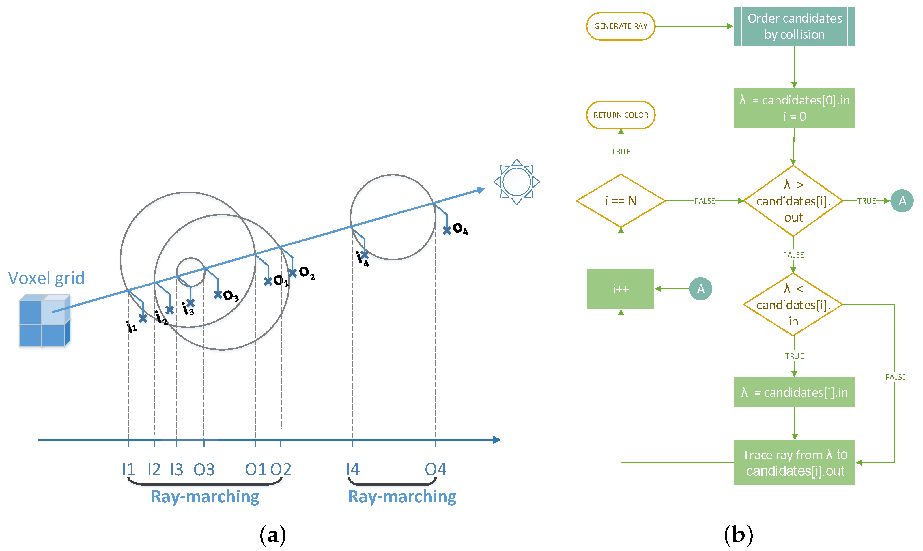
Figure 5.
Graphical and procedural explanation of the no duplicate tracing algorithm. (a) A basic model that illustrates the zones to sweep. In this case only I1 to O2 and I4 to O4 are traced following the ray; (b) A flow chart illustrating the the no duplicate tracing algorithm (Algorithm 2).
Figure 5.
Graphical and procedural explanation of the no duplicate tracing algorithm. (a) A basic model that illustrates the zones to sweep. In this case only I1 to O2 and I4 to O4 are traced following the ray; (b) A flow chart illustrating the the no duplicate tracing algorithm (Algorithm 2).
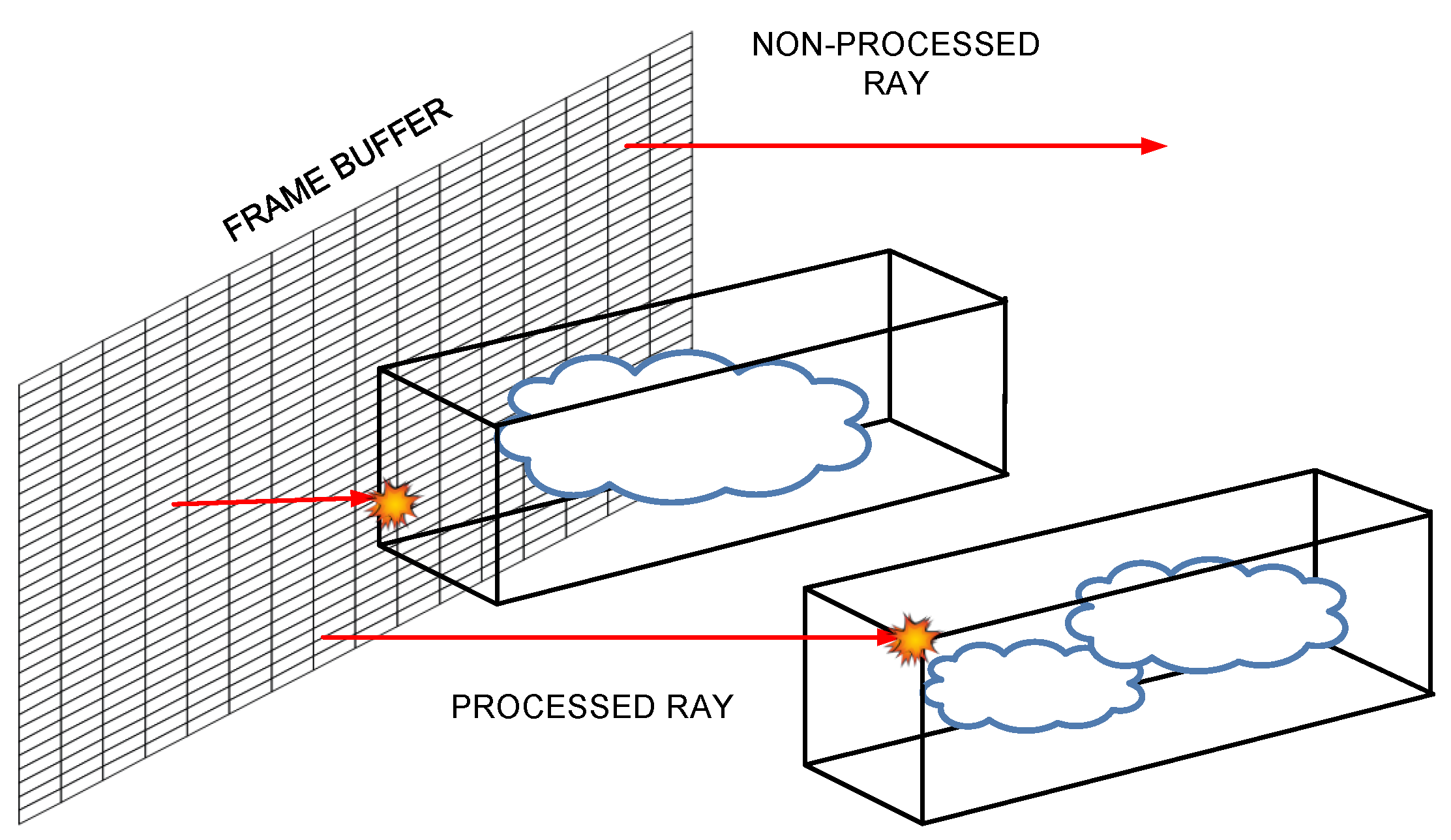
Figure 6.
Bounding box delimitation of clouds. Smits’ algorithm is useful for optimizing ray-marching by calculating the segment of the Euclidean straight line along which rendering must be performed according to the value.
Figure 6.
Bounding box delimitation of clouds. Smits’ algorithm is useful for optimizing ray-marching by calculating the segment of the Euclidean straight line along which rendering must be performed according to the value.
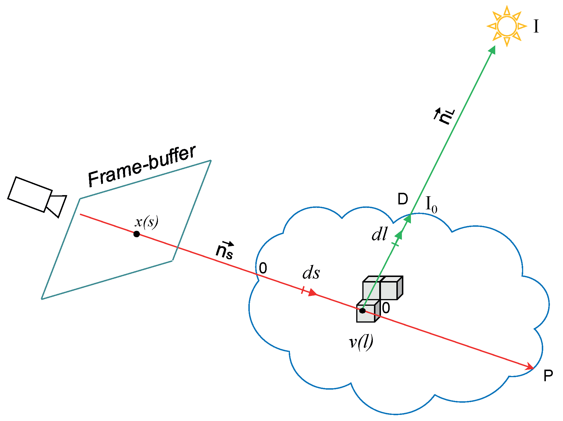
Figure 7.
A two-pass algorithm for lighting along ray l and rendering along ray s. and are the direction vectors of the ray-marching and the light respectively. and are the processing dimensions of line integral in the cloud for ray-marching and light respectively. is frame-buffer pixel and is a point into a voxel.
Figure 8.
A three-dimensional Gaussian distribution. Some cloud shapes resemble a 3D Gaussian normal distribution, specifically the cumuliform ones. The cause is the altitude at which the condensation is produced. Since the condensation level may be conceived as a flat and horizontal surface, the clouds formed at this level have a flat bottom side, as cited by Häckel’s book [
34].
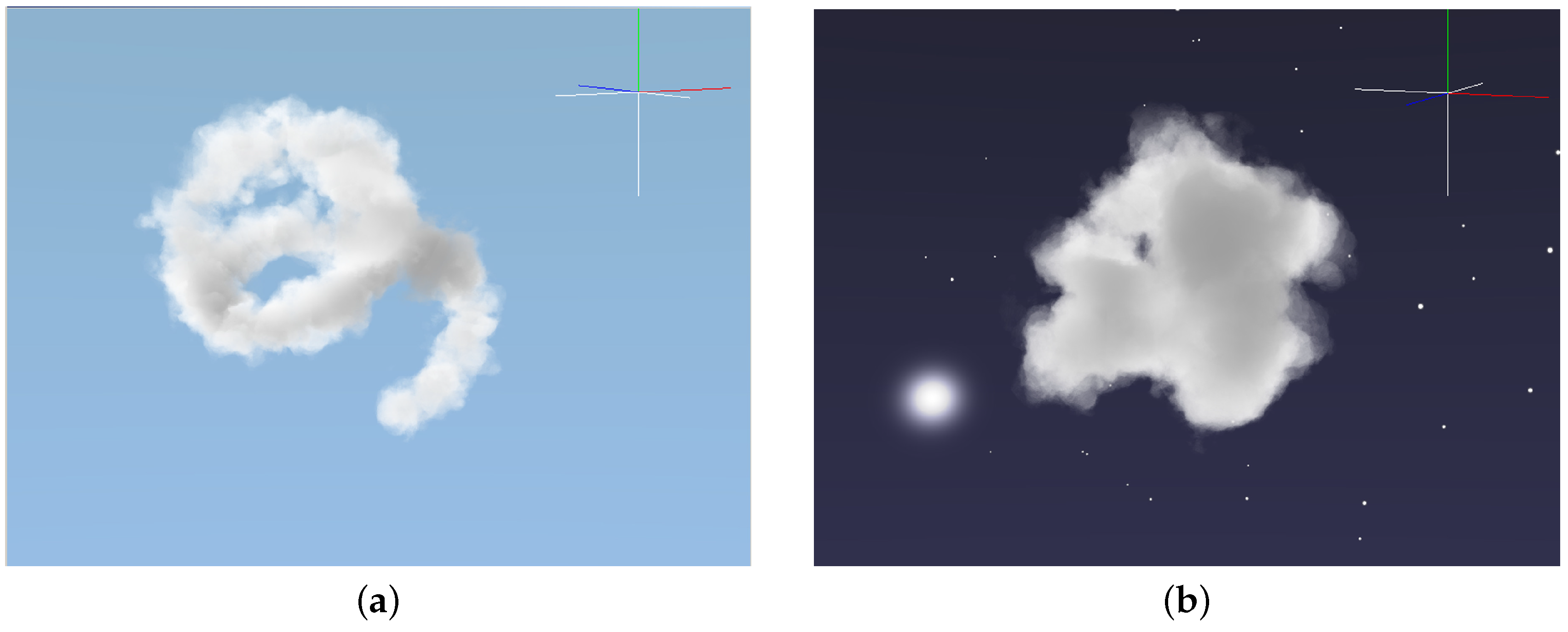
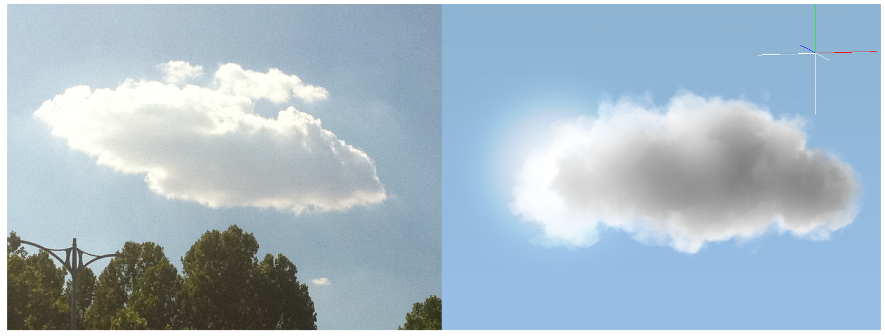
Figure 9.
Example of clouds with Gaussian distribution. A real photograph (left) and our generated cumulus (right) using 35 pseudo-spheroids in total.
Figure 9.
Example of clouds with Gaussian distribution. A real photograph (left) and our generated cumulus (right) using 35 pseudo-spheroids in total.
Figure 10.
A crepuscular landscape with three Gaussian cumuli executing the volumetric scattering and voxel shading with cloud interaction and occlusion.
Figure 10.
A crepuscular landscape with three Gaussian cumuli executing the volumetric scattering and voxel shading with cloud interaction and occlusion.
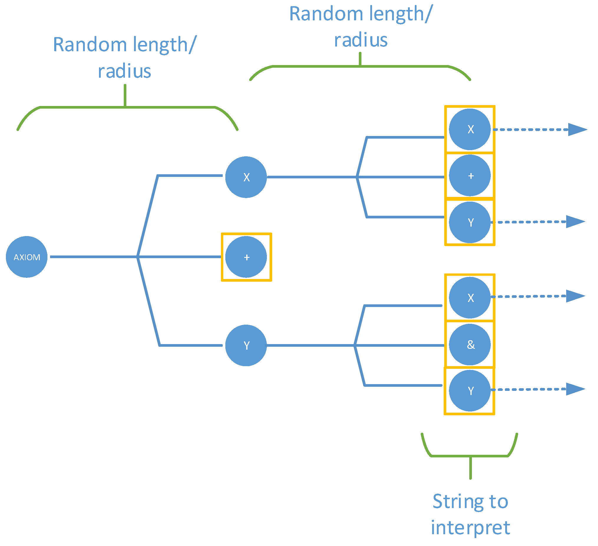
Figure 11.
After each recursive call, the interpreter generates a new proportional random radius and length for the primitives. This produces more natural and impressive cumuliforms.
Figure 11.
After each recursive call, the interpreter generates a new proportional random radius and length for the primitives. This produces more natural and impressive cumuliforms.
Figure 12.
Generated clouds from the previous L-system grammar derivation. (a) Iterations = 7, = 10°. The lower the angle , the thinner and more strange the cloud shape becomes, hence the cloud looks like a 3D spiral. This is caused by the recursive turning operators in the grammar productions that respond to the director rotation angle and the uniform random sphere radius; (b) Using exactly the same grammar and iterations with a larger angle, for instance [50°, 100°], the resulting grammar derivation generates dense cumulus formations.
Figure 13.
Different cumulus formations using a Gaussian distribution and optimized metaballs. Just six spheres were used to render the samples by randomizing the sphere radius.
Figure 13.
Different cumulus formations using a Gaussian distribution and optimized metaballs. Just six spheres were used to render the samples by randomizing the sphere radius.
Figure 14.
(a) Ellipsoid scaling process. The proposed algorithm multiplies each triangle vertex () by a factor that typically falls in the range (0.1, 2], once the barycenter (B) is calculated. Afterwards, the shader algorithm uses the maximum distance from the barycenter to the scaled triangle vertex to estimate the density in the ellipsoid/ray collision equations; (b) After rotation. As seen in the image above, showing the original ellipsoid in black and the resulting one in green, the previous equations allow overlapping of the direction vectors. Hence, according to the direction of the larger triangle vertex, the algorithms produce the resulting rotation.
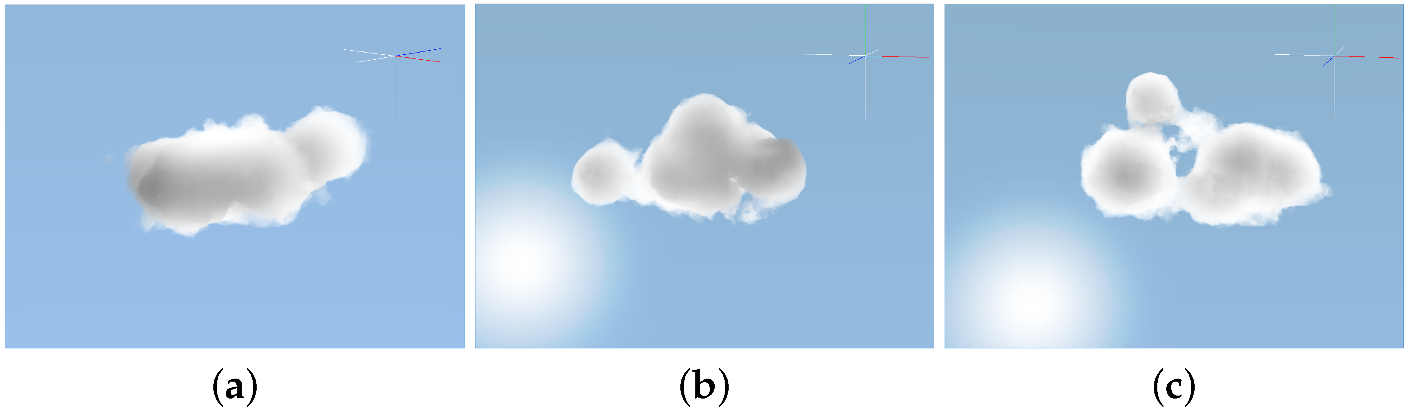
Figure 15.
Example of 3D meshes converted to cumuliform clouds resembling known shapes. (a) A hand mesh transformed into a soft 3D cloud. The final result is successfully optimized for real-time GPU algorithm animation and rendering; (b) A rabbit mesh with 370 triangles. 80% decimation has been performed on this mesh, reducing the number of triangles from 1850 to 370 to achieve a suitable real-time performance.
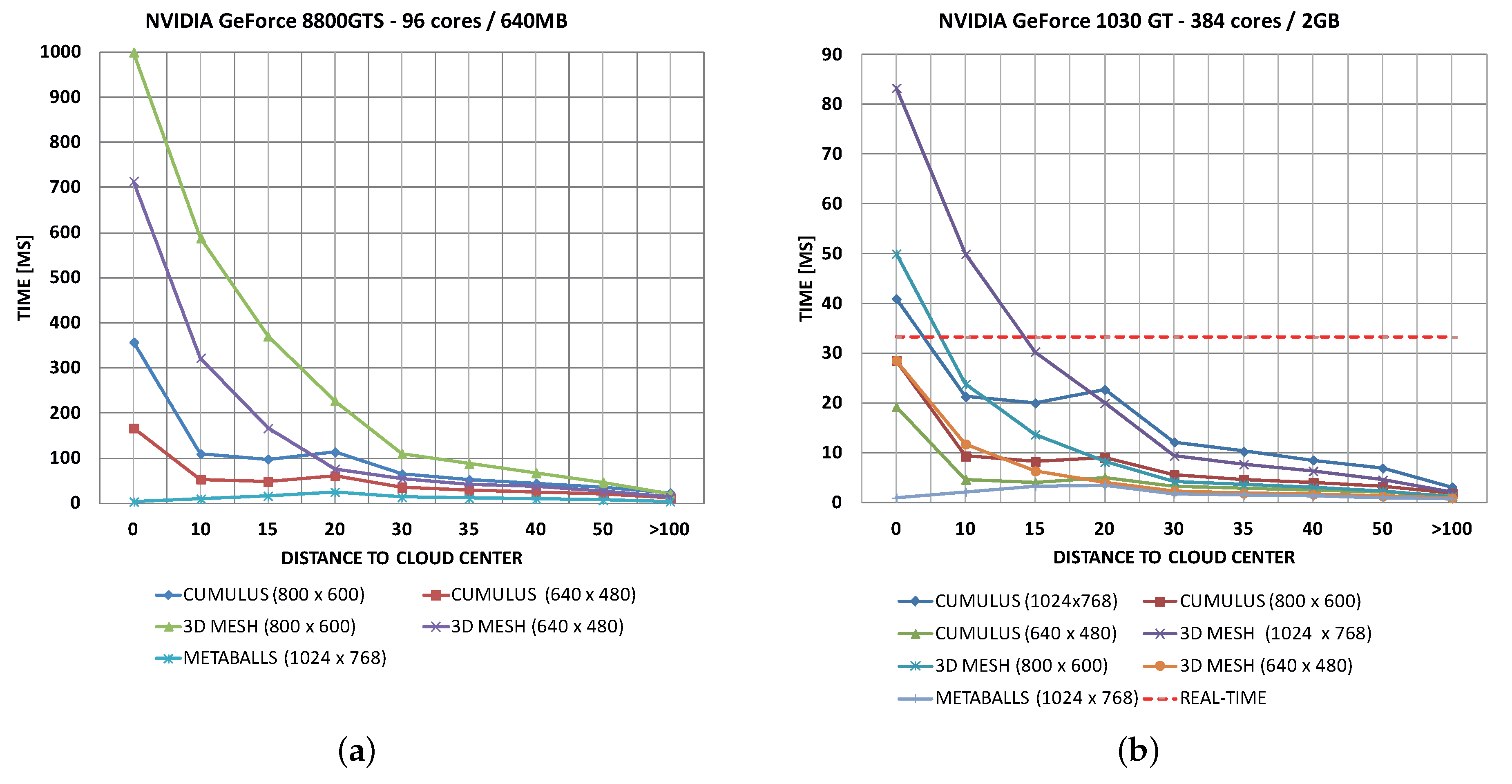
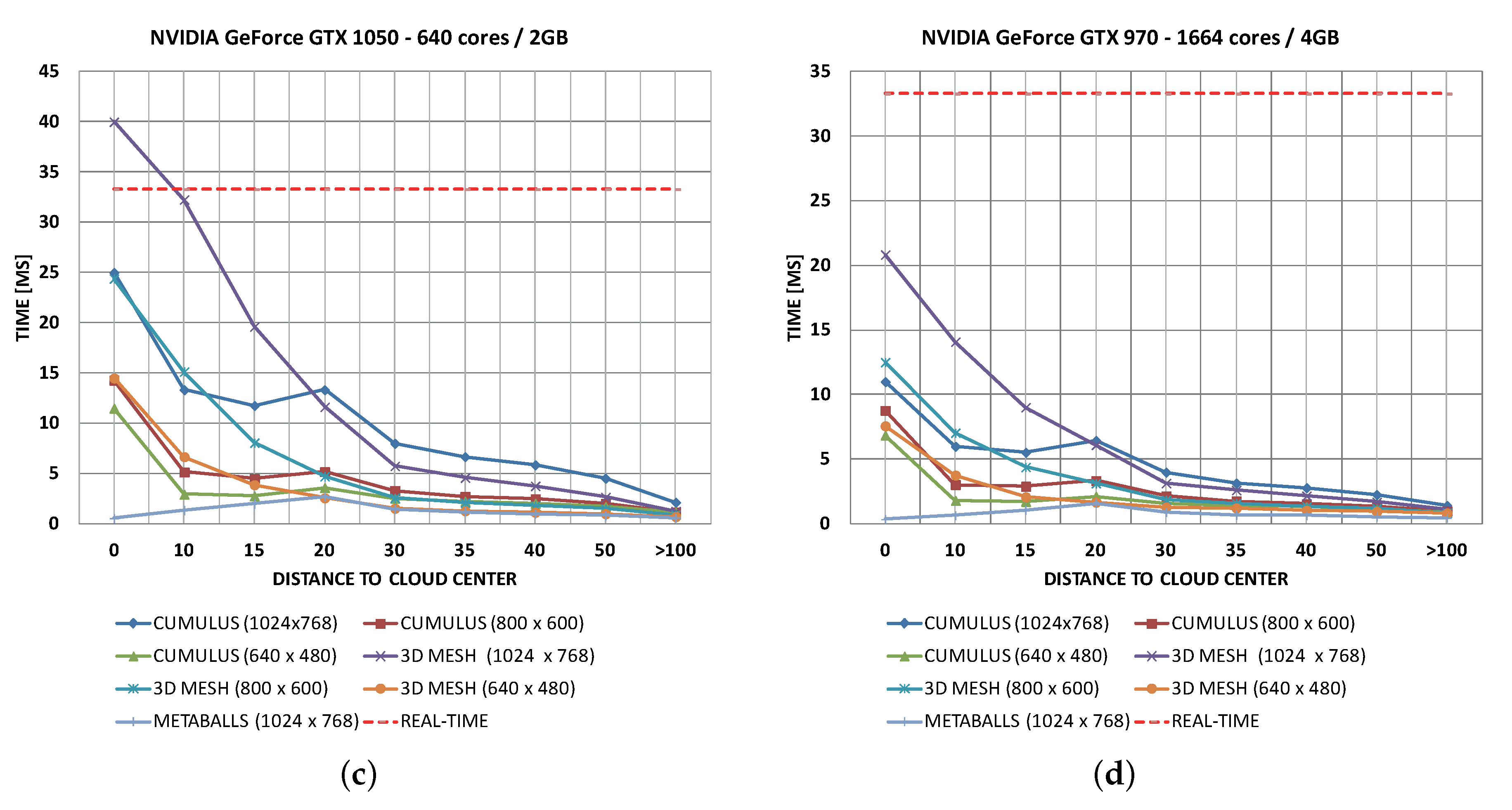
Figure 16.
The performance of the algorithms on different graphic cards. (
a) With the GeForce 8800 GTS, the performance at 800 × 600 pixels overcomes the limit of the hyper-realistic method shown in Reference [
40]; (
b) With the GeForce 1030 GT, the performance is optimum in most cases, except when the level of detail (LOD) equation is manually bypassed to force higher quality; (
c) Performance in a GeForce GTX 1050 is optimum in 99% of cases; (
d) Based on empirical tests in a GeForce GTX 970, the proposed model achieves a geometric frame rate increment in all algorithms. Results are very promising for the both cumulus and 3D mesh tracing algorithms in all resolutions, including full-HD.
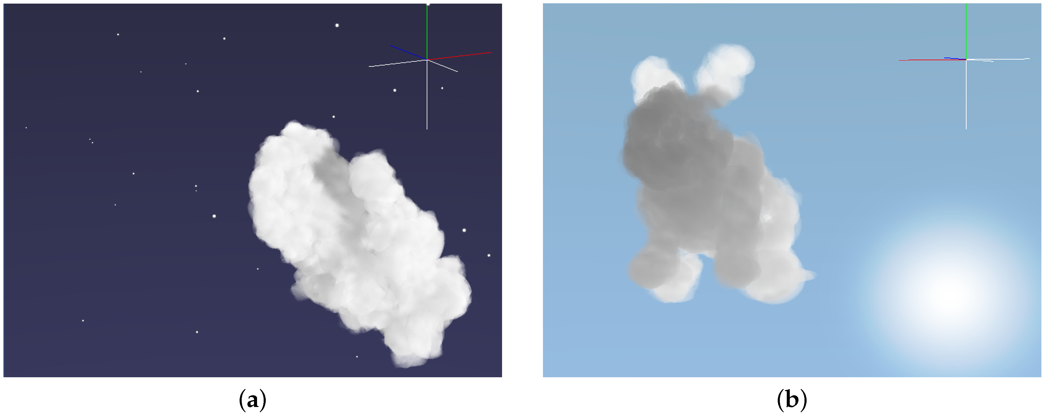
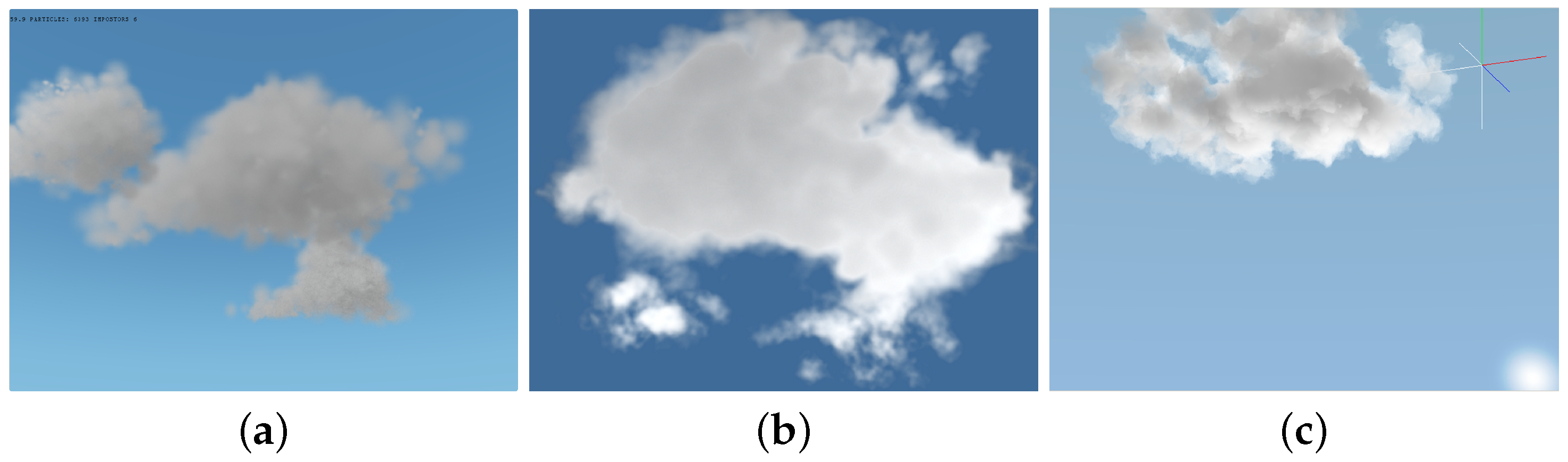
Figure 17.
Differences between our model and other works. (
a) A generated cloud using the particle systems of Harris [
13], and Huang et al. [
1]. The contour of the cloud and the overall realism lack accuracy. (
b) The cloud modeling method of Montenegro et al. [
41] that combines procedural and implicit models. (
c) Our ontological volumetric cloud rendering method with lighting. The procedural noise improves cloud edges and fuzzy volume effects.
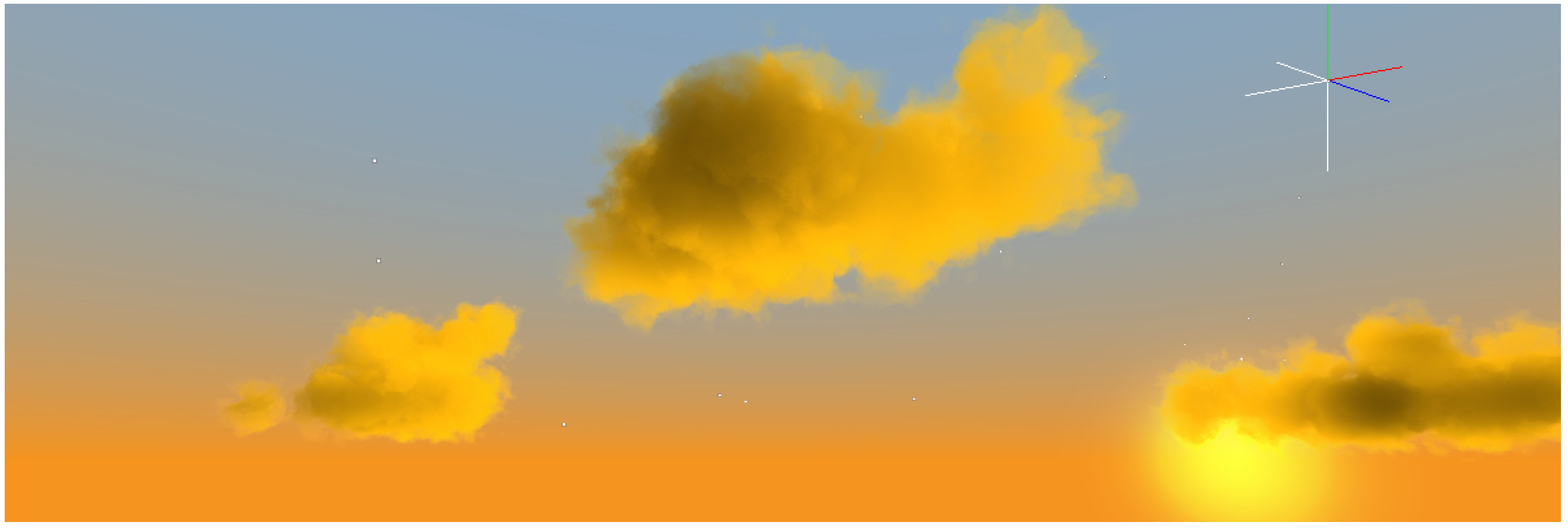
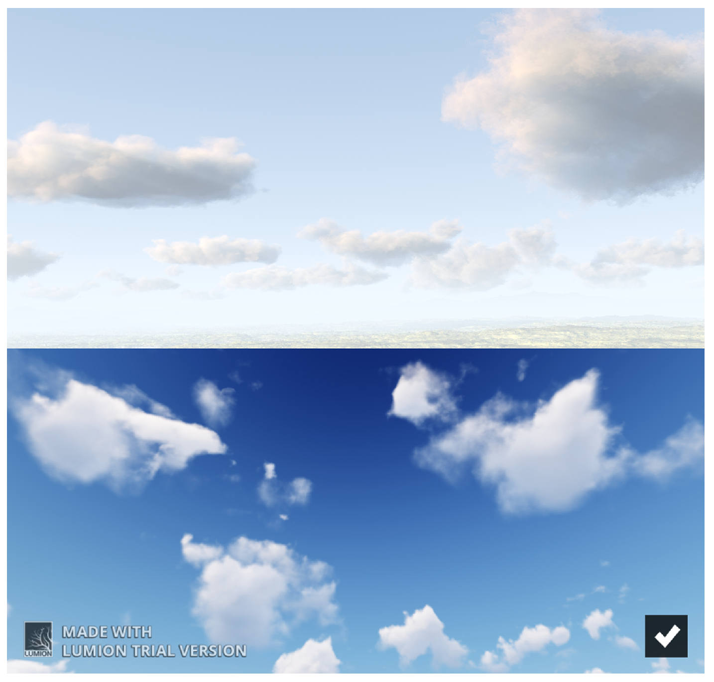
Figure 18.
Photo-realistic clouds with all physical characteristics. The image above was generated with POV-Ray in 1 h, 18 min using 100% of the CPU cores at 1024 × 768 pixel resolution. The image below was generated with Lumion 7.5 taking around 1 s for the skydome texture. These are antithetical model examples that differ from the real-time system explained in this paper.
Table 1.
Pros and cons of each method.
Table 1.
Pros and cons of each method.
| Texturized Primitives | Particle Systems | Geometry Distortion | Volumetric Rendering |
|---|
| Procedural | ✔ | ✗ | ✗ | ✔ |
| Animation | ✗ | ✔ | ✔ | ✔ |
| Traverse | ✗ | ✔ | ✗ | ✔ |
| Interactive | ✔ | ✔ | ✔ | ✔ |
| Turn around | ✗ | ✔ | ✔ | ✔ |
| All kind of clouds | ✔ | ✗ | ✗ | ✔ |
| Realism | ✔ | ✗ | ✔ | ✔ |
| Performance | ✔ | ✔ | ✔ | ✗ |
| State-of-the-art | ✔ | ✗ | ✗ | ✔ |
Table 2.
Typical parameters for our Gaussian equations where , t and are scale constants.
Table 2.
Typical parameters for our Gaussian equations where , t and are scale constants.
| Axis | | | Clamped |
|---|
| X | | | [] |
| Y | | | [,] |
| Z | | | [-] |
Table 3.
The table below shows the minimum distance from the cloud at which full high-definition (HD), 1920 × 1080 pixels, rendering reaches 30 frames-per-second (FPS, minimum real-time). This distance is suitable for scenarios where getting close to the surface of the cloud is required.
Table 3.
The table below shows the minimum distance from the cloud at which full high-definition (HD), 1920 × 1080 pixels, rendering reaches 30 frames-per-second (FPS, minimum real-time). This distance is suitable for scenarios where getting close to the surface of the cloud is required.
| Card/OpenGL Euclidean Distance | Cumulus | 3D Model |
|---|
| GT 1030 | | |
| GTX 1050 | | |
| GTX 970 | | |
Table 4.
Average frequency of other particle and volumetric systems compared with our method.
Table 4.
Average frequency of other particle and volumetric systems compared with our method.
| Huang et al. | Montenegro et al. | Kang et al. | Yusov | Bi et al. | Our method |
|---|
| FPS | 99.5 | 30 | 60 | 105 (GTX 680) | 50 | >150 (GTX 1050 non-Ti) |


