Multi-Source Stego Detection with Low-Dimensional Textural Feature and Clustering Ensembles


1
College of Computer Science and Technology, Shanghai University of Electric Power, Shanghai 200090, China
2
Computer Science Department, University of Victoria, Victoria, BC V8W 3P6, Canada
3
School of Communication and Information Engineering, Shanghai University, Shanghai 200444, China
*
Author to whom correspondence should be addressed.
Symmetry 2018, 10(5), 128; https://doi.org/10.3390/sym10050128
Submission received: 1 March 2018
/
Revised: 9 April 2018
/
Accepted: 17 April 2018
/
Published: 24 April 2018
(This article belongs to the Special Issue Information Technology and Its Applications 2021)
Abstract
:This work tackles a recent challenge in digital image processing: how to identify the steganographic images from a steganographer, who is unknown among multiple innocent actors. The method does not need a large number of samples to train classification model, and thus it is significantly different from the traditional steganalysis. The proposed scheme consists of textural features and clustering ensembles. Local ternary patterns (LTP) are employed to design low-dimensional textural features which are considered to be more sensitive to steganographic changes in texture regions of image. Furthermore, we use the extracted low-dimensional textural features to train a number of hierarchical clustering results, which are integrated as an ensemble based on the majority voting strategy. Finally, the ensemble is used to make optimal decision for suspected image. Extensive experiments show that the proposed scheme is effective and efficient and outperforms the state-of-the-art steganalysis methods with an average gain from to .
1. Introduction
Steganalysis, as a countermeasure for steganography, aims to detect the presence of hidden data in a digital media, such as digital images, video or audio files. Since steganography hides data into the image elements (pixels or DCT (Discrete Cosine Transform) coefficients), the distribution of image modes usually change slightly after steganography. In most steganalytic techniques [1,2,3,4], one can extract sensitive feature sets (low-dimensional [5,6] or high-dimensional [7,8,9,10,11]) from large datasets of digital images, which include original and steganographic images. These features are used to train a classifier that can separate a suspected image as cover (original image) or stego (steganographic image).
In traditional steganalytic techniques, however, the problem of detecting hidden data is usually restricted in scenarios where only a single actor (or equivalently a user) is considered, i.e., to detect whether or not objects from the same user are cover or stego. We call this problem as the stego detection problem. In many real-world scenarios, particularly in social media networks, such as Flickr [12] and Instagram [13], that include millions of users sharing images, solutions to stego detection becomes infeasible since we do not know the culprit users beforehand [14,15,16]. As such, we need to detect which users are suspicious of using steganography to deliver hidden information. This new problem is termed as the steganographer detection problem and has been recently studied in [14,15,16,17].
Aiming at the stego detection problem, three different steganalytic schemes based on supervised learning have been presented. In the first scheme, steganalyzers are assumed to be able to estimate the payload length [18,19,20] for some simple steganographic methods, such as JSteg [21] and least significant bits replacement (LSBR) [22]. These schemes usually achieve an overall good performance. However, they rely on a local autoregressive image model and usually assume that the algorithm has been known before hand. In the second scheme, more sophisticated features are extracted from cover or stego images to obtain accurate detection [6,8,9,10]. In this scenario, efficient detectors employ a lot of samples to train classification model and make a binary judgement for testing sample. This type of methods can effectively defeat the state-of-the-art steganographic methods, such as EA (Edge-Adaptive) algorithm [23], HUGO (Highly Undetectable steGO) [24], WOW (Wavelet Obtained Weights) [25], and Spatial UNIversal WAvelet Relative Distortion (S-UNIWARD) [26]. Nevertheless, the performance of this type of methods is sensitive to model mismatch. Hence, one needs lots of images from the same source to correctly train the classifier. Unfortunately, such data might be impossible to access in social networks. In the third scheme, steganalizers employ statistical distribution of image mode (DCT coefficients or pixels) to build a model, which is used to design detector by statistical hypothesis testing [27,28,29]. In this scheme, however, statistical distribution parameters need to be learned by a large number of samples and an improper cover image model may result in overall poor detection performance.
Aiming at the steganographer detection problem, researchers try to employ unsupervised learning methods to solve this problem. Unsupervised learning is used to train a classifier which can separate “outliers” as steganographer from multiple innocent ones [14,15,16,17]. It has been shown that all the three schemes for the stego detection problem do not work well for steganographer detection [16], and only Ker’s method [14,15,16] and Li’s method [17] are applicable. Unfortunately, existing solutions to the steganographer detection problem can only identify a potential steganographer but cannot pin down to the steganographic images from the steganographer. This is because these solutions explore the statistical features extracted from all images of an actor and detect the outlier actors as potential steganographers.
One natural question arises: could we adopt a two-step procedure to effectively identify the steganographic images when the source images are from many users? The two-step procedure first uses steganographer detection [14,15,16,17] to find potential steganographers and then applies existing stego detection methods to discover steganographic images.
Unfortunately, the answer is negative due to the following two pitfalls in the above two-step procedure. First, existing stego detection methods usually employ massive samples from the same source to train a generalized model, which is used to classify a suspected image as cover or stego. Unfortunately, such massive training images from the same source (or user) are not easy to find in real-world social media networks. Second, even if the generalized model can be obtained, it does not always match well for unknown image database from other sources, and thus may lead to high false positive and incorrect accusation.
This paper is thus motivated to tackle the following challenge: stego detection in the context of real-world social media networks where image sources could be from many users. We term this new problem as multi-source stego detection problem, which poses a special challenge to digital image processing due to the above reasons. We tackle this problem with (1) low-dimensional textural features and (2) clustering ensemble applied to multi-source steganographic targets. In the former, we develop the local ternary patterns to design high-dimensional textural feature set, whose dimension is subsequently reduced to an appropriate level according to feature correlation. In the latter, for a group of suspected images, multiple sub-image sets are set up by a cropping procedure. Each sub-image set returns a decision (identifying suspected image) with hierarchical clustering. Subsequently, an ensemble is built by a majority voting strategy. The proposed scheme does not need a lot of training samples to train the generalized model, so, it is significantly different from existing solutions to the stego detection problem and can address successfully the problem of detecting steganographic images when the source images are potentially from many users. Comprehensive performance tests are performed with a lot of real-world images from a series of cameras and experimental results demonstrate that with the help of low-dimensional textural feature set and clustering ensemble, our proposed approach shows a significant advantage over the traditional steganalysis methods in the context of multi-source stego detection.
The rest of this paper is organized as follows. Section 2 reviews existing unsupervised steganalysis methods applied for steganographer detection. In Section 3, we provide detailed procedures of forming low-dimensional textural features with local texture pattern and then introduce the method of constructing hierarchical clustering and ensemble strategy. Subsequently, comprehensive experiments are performed to evaluate the performance of proposed scheme. The corresponding experimental results and discussions are presented in Section 4. Finally, Section 5 concludes the paper.
2. Related Work
2.1. Local Pattern Feature
Adaptive steganographic schemes usually enforce embedding changes in texture regions of an image. Steganalysis features using local binary pattern (LBP) have been adopted in [10]. LBP operator selects a local neighborhood around each pixel. It thresholds these neighborhood pixels at the value of the central pixel and uses the resulting binary-valued region as a local image descriptor. LBP is originally defined for neighborhoods, and then gives 8 bit integer based on the 8 pixels around the central pixel. Thus, a histogram of 256 bins is formed as the texture descriptor, which includes important information about spatial structure of image texture.
Nevertheless, due to the exact threshold for the value of the central pixel, LBP features are not sensitive to the steganographic changes, especially in the texture regions of image. Inspired by LBP features, researchers developed local textural features (LTF) to design steganalysis features [4] and then reduce the dimensionality of feature set by employing double principal component analysis (DPCA). However, since this scheme contains two dimensionality reduction procedures, the time complexity significantly increases, and more importantly, the efficiency of feature set may be affected due to the loss of feature attributes including significant classification information. Thus, efficient dimensionality reduction method should be exploited to design more sensitive low-dimensional feature sets.
2.2. Steganographer Detection
Traditional image steganalysis methods usually need massive images as training database to train a general model. Then, suspected images (i.e., test images) are classified by using this model. In these methods, however, the training images and test images are assumed to be from the same image source. Unfortunately, in many real-world scenarios, there may not exist sufficient training images from the same source. As a result, the trained model may not match well the features of test images, leading to poor detection results. To avoid the problem, steganalysts try to use cluster analysis [14,17] or anomaly detection [15,16] to solve this problem.
Ker et al., proposed two steganalysis schemes for detecting steganographers (or actors) using Maximum Mean Discrepancy (MMD) [30]. In their methods, classical feature vector, PEV-274 feature vector [5], was used to represent an image. Notably, the raw features may have different scales that can significantly impact the detection accuracy, and as such the extracted features need to be normalized. Generally, assume that there are l actors, each having m images. By normalization, each dimensional feature is scaled to have zero mean and unit variance, that is, and , where is the normalized version of the raw feature set . Since the feature vectors arise from a probability distribution that characterizes the actors’ cover image source or their stego source, Ker et al., considered MMD as a measure of similarity between probability distributions and used it to compare the feature vectors of two actors. MMD corresponds to an distance in a Hilbert space implicitly defined through a positive definite kernel function , where x and y are d-dimensional feature vectors. The kernel function k may be of different forms, including the linear kernel and the Gaussian kernel , where is the inverse kernel width. A sample estimate of the MMD distance can be calculated as:
Ker et al., used MMD to calculate the distance between each pair of actors and then gave two detection schemes for suspected actors: (1) Use hierarchical clustering to group users incrementally and consider the smaller cluster from the last two clusters as the suspected actors; (2) Use an outlier detection algorithm, called Local Outlier Factor (LOF), to rank each actor according to the degree of anomaly and consider the actors at the top ranks as suspected actors. Ker’s two schemes have shown promising performance in solving the steganographer detection problem.
On the basis of Ker’s schemes, Li et al., presented a new solution [17] by using high-order joint features and ensemble scheme to further improved the performance of steganographer detection. High-order joint matrices of DCT coefficients of JPEG images are built to present new steganalysis feature set. In addition, an ensemble scheme with majority voting strategy was introduced in hierarchical clustering to improve the detection accuracy. Since single clustering is unstable and there is no clustering method capable of correctly identifying the underlying structure for all data sets, Li’s scheme is more robust than the single-round clustering and leads to an significant improvement.
The above-mentioned methods, Ker’s schemes and Li’s scheme, all try to identify the steganographer. Nevertheless, it is not enough for only identifying the suspected steganographer in social networks. It is also important to pin down to the steganographic images from a suspected steganographer. Therefore, we need to exploit more sensitive features to accurately reflect the distance between two images. This paper is to fill this gap.
3. Proposed Steganalysis Scheme
3.1. The Framework of Proposed Scheme
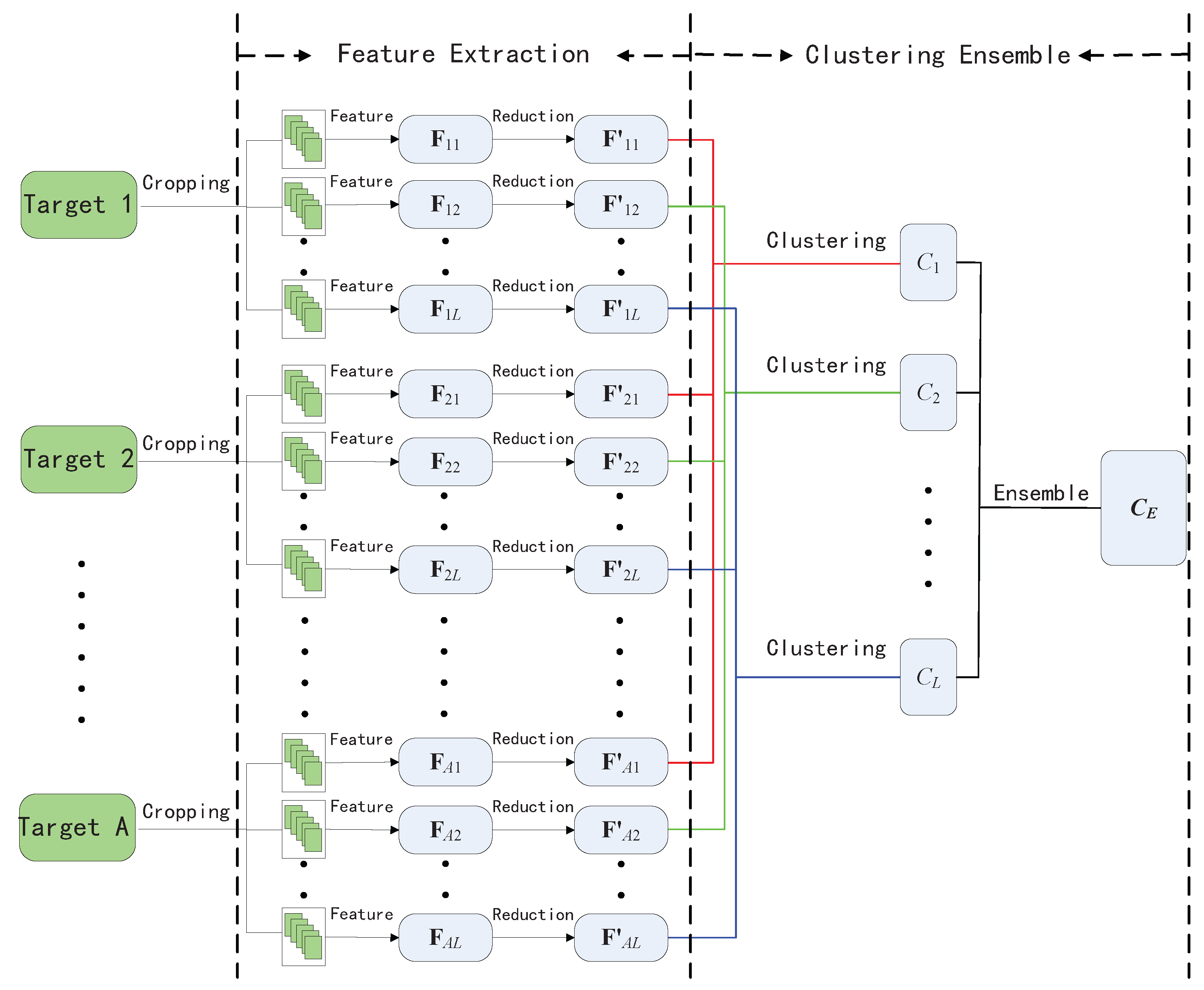
The framework of our proposed scheme is shown in Figure 1. Proposed steganalytic scheme is comprised of two parts: textural feature construction and clustering ensemble. In the former, we calculate a low-dimensional textural feature vector from sub-images which are sampled from individual bigger image. In the second part, majority voting-based ensemble mechanism is introduced into hierarchical clustering to identify the suspected steganographic image as cover or stego.
3.2. Low-Dimensional Textural Features for Steganalysis
In this section, we firstly use different filters to calculate multiple residual images, and then employ the local ternary pattern to construct a high-dimensional original feature set. Subsequently, inspired by the Huffman coding [31], we further perform dimensionality reduction procedure for the high-dimensional original feature set. Finally, a low-dimensional textural feature set can be obtained by merging feature vectors with major correlation coefficient.
3.2.1. Obtaining Residual Image with Filters
Since steganography usually embeds data into image modes (pixels in spatial images or DCT coefficients in JPEG images) so that they are modified slightly, these small perturbations may be considered as a high frequency additive noise, and can be effectively revealed by the residual image after eliminating low frequency representation. In this section, we obtain a series of residual images by using different filtering processes.
Denote as original image, as residual image, and Pred() as corresponding predicted image. Given an image, we obtain six residual images with the following processing.
- (1)
- Residual images based on difference filtering. With Equation (2), four residual images are directly calculated along the horizontal, vertical, main diagonal, and minor diagonal directions, respectively.
- (2)
- (3)
- Residual images based on law’s masks. A residual image is formed by using a 3 × 3 mask in original image, which is shown in Figure 2b.
3.2.2. LTP-Based High-Dimensional Textural Feature
In this section, we extract high-dimensional textural feature set based on LTP, which is constructed with a 3-valued code. A zone with width around the central pixel is determined in a region. For the eight neighboring pixels of , the grayscale levels are quantized to 0 if they are in this zone, 1 if they are above this zone, and 2 if they are below this zone. In general, LTP is expressed by the following form
where
In Equation (6), a specific threshold t is used to control the sensitivity of LTP descriptors to noise and grayscale-level changes. Here, the threshold t is set to 3. LTP features are obtained from the histogram of LTP values, which are in the interval . Obviously, we can extract dimensional features from a residual image. Extracted textural features have dimensions, where 6 is the number of residual images.
Notably, with Equation (2), we can extract dimensional features by four residual images calculated from horizontal, vertical, main diagonal and minor diagonal directions. We consider the average of horizontal and vertical, and the average of main diagonal and minor diagonal, respectively, to reduce the dimensionality to . Together with the feature from the average filtering process (6561 dimensions) and the feature from the law’s mask process (6561 dimensions), the final textural features thus have dimensions.
3.2.3. Dimensionality Reduction
Obviously, the extracted textural features have a rather high dimension and each feature vector includes a lot of zero (or close to zero) values. This leads to strongly-correlated and redundant features so that the classification performance of features becomes rather weak. To solve the problem, we adopt the similar idea of Huffman coding [31] and calculate the correlation coefficient between feature vectors and perform dimensionality reduction by merging feature vectors with major correlation coefficient to improve classification performance of textural features. Notably, our proposed dimensionality reduction procedure can only process 6561 dimensional features each time. Since the designed textural features in Section 3.2.2 have dimensions, this reduction procedure must be repeated 4 times in order to cover the whole set. The merging processes are as follows.
Assume that the feature set includes N samples from k different users, , where k is the number of users and represents the number of samples from k-th user. We extract 6561 features from each sample according to local ternary patterns to form a high-dimensional textural feature set as , where . To remove the redundant feature vector, we firstly calculate the correlation coefficient between any two feature vectors and by the following equation:
where . In the right side of the equation, the numerator stands of the covariance of and , while the two terms of the denominator represent their standard deviations, respectively. The average correlation coefficient between s-th feature vector and the others can be calculated by
where M is the dimension of current feature set and . The average correlation coefficient of each feature vector can be calculated by the above calculations. Furthermore, the features with major correlation coefficients are merged incrementally to reduce the dimensionality. Denote the extracted feature set , the merging procedure is as follows.
For current feature set, calculate the average correlation vector by Equations (7) and (8), where M is the dimension of current feature set.
Introduce an ascending permutation function to sort the correlation vector such that , where . Then, sort the feature set by using the same function . The sorted feature set is denoted as .
Merge two feature vectors and by Equation (9) as new vector to replace the original vectors in . Meanwhile, and in will be removed. The merged feature set is denoted as .
For merged feature set , repeat Steps 1 to 3 until the dimension of feature set reducing to d dimensions, where d is a tuning parameter.
Obviously, d is utilized to control the dimensionality of textural features. Figure 3 shows the performance of textural features with different parameter d. In this experiment, experimental images are from the classical BOSSbase 1.01 database [32] which contains grayscale images with size of . We choose entire BOSSbase and use Gaussian Support Vector Machine (G-SVM) classifier [33] in our experiment. Two state-of-the-art steganographic algorithms, Edge-Adaptive (EA) [23,34] and Highly Undetectable steGO (HUGO) [24,34], are employed, and the relative payloads are set as bit per pixel (bpp). When we hide messages in BOSSbase, the corresponding images after embedding data are denoted as stego images. We randomly select 6000 cover images and their corresponding 6000 stego images as training set, while for the remaining 8000 images, including 4000 cover images and their corresponding stego images, we randomly select 4000 images as testing set, which may be composed of different number of covers and stegos (there is not a consistent one-to-one match between each cover and stego). The experiments are repeated 20 times to show the average error probability . In Figure 3, the x-axis represents parameter , while the y-axis represents the average error probability , where and stand for the probability of false positive and probability of false negative, respectively. In our test, quickly drops to the minimum and then grows slowly with the increasing d. The optimal value d is about 112 where a minimal occurs whatever the payload is. In the end, we reduce the dimension of features from to .
3.3. Clustering Ensemble
Furthermore, we propose an ensemble strategy with hierarchical clustering to effectively identify steganographic target by assuming that the majority of images are innocent. First, individual image is randomly cropped with smaller size to build sub-image sets. Textural features mentioned in Section 3.2 are extracted from these sub-image sets. After performing the agglomeration hierarchical clustering in textural feature space, a suspected image can be separated from the innocent ones. By repeating the above steps, multiple decisions can be made, and the final steganographic images are decided with majority voting in the multiple decisions.
Denote a set of A images as , which includes steganographic and innocent images. Clustering ensemble is used to separate the steganographic images from other innocent ones by the following steps.
Randomly crop each image to size in . The cropped images consist of A image subset , where includes B images of size .
For each image subset , extract the textural features using the method introduced in the previous section to form feature sets , where , B denotes the number of times that the image is cropped in Step 1, and each represents a 448-dimensional feature vector.
Normalize the feature sets such that every column of feature matrix has zero mean and unit variance. Then, the distance between different pairs of feature sets can be calculated by using MMD with Gaussian kernel, which is shown in Equation (1).
Perform hierarchical clustering with the MMD distance measure. First, two sub-image sets with the minimal distance are combined into a new cluster, denoted as , and the remaining sub-image sets are in a set denoted as . We then repeatedly select a feature set from and add the selected set into until only one set left in . At each selection step, the image subset that has the smallest distance to is selected, where the distance between an image subset and a cluster is defined as:
The last remaining image subset in consists of the cropped smaller images from an image, which is considered to be the suspected image.
Repeat Steps 1~4 L times. Each time, we identify a suspected image and denote it as . By majority voting on the L detections, the image that is labeled as suspicious the most times is determined to be the final detection result. When there is a tie, randomly select one to break the tie.
Notably, the two parameters m and n have a major impact on the detection accuracy, which will be discussed in the experimental section. In addition, we would like to point out that ensemble strategy will work only if the individual sub-clusterings are sufficiently diverse. In other words, the success of ensemble strategy mainly relies on the instability of based learners (sub-clusterings), because they can make different errors on unseen data. If the original images have diverse content and the cropped size is suitable, there will be much diversity in the randomly-cropped images so that each sub-clustering tends to generate different results. In this sense, the benefit of ensemble will be clear.
4. Experimental Results and Discussion
In our experiments, we validate the proposed scheme by simulating a situation similar to a real-world social network. Different social scenarios that one or zero stegnographic images hide in multiple innocent ones from different users are simulated. Our goal is to detect these stegnographic images.
To simulate the proposed steganalytic scheme, we design an experiment in which one or zero images are selected as the steganographic images and mixed in multiple innocent ones from different actors. The proposed stego detection method is run to identify the steganographic image. We firstly need to judge whether all images are innocent, if not, we further pin down to the suspected images. In our experiments, each experiment is run 100 times to obtain an average result, which is considered to be the overall performance evaluation. We select a different image as the steganographic object each time, which is embedded with messages of different total relative payloads by the four steganographic algorithms introduced in the previous section. The overall identification accuracy rate (AR) is calculated as the number of correctly detection over the total number of detection, i.e.,
Since the performance is influenced by the number of clusters [16], we randomly select no more than 20 images () and each image is cropped 50 times () in each run to investigate the impact.
4.1. Experimental Setup
4.1.1. Image Source
In this work, we carry out the experiments on a simulated image database, which contains 4636 images acquired by seven digital cameras. These cameras are with different noise models so that they can be used to imitate different image sources. Table 1 shows the details from seven camera model with different native resolution and quantity.
In order to assure reproducibility of experiments, it is important to include as much information about the image source as possible. As such, the experimental images are firstly captured with the RAW format (CR2 or DNG) (We do not consider the compressed image source, because it may remove high frequency noise of images and produce influence for the proposed textural features.). Subsequently, they are converted to 8-bit grayscale, and resized using bilinear interpolation so that they have the approximately (To ease comparison, we implement unified processing with the minimal resolution in seven cameras.) same size of .
The images belong to diverse categories, including people, animals, landscape, flowers, foods, and so on. For each experiment, one camera is selected to simulate a “steganographer” (user or actor) in social networks. We choose some images from this simulated “steganographer” to form test set, which may be embedded with messages by different steganographic algorithms.
4.1.2. Steganographic Algorithms
We test the following four steganographic algorithms: Edge-Adaptive (EA) [23,34], Highly Undetectable steGO (HUGO) [24,34], Wavelet Obtained Weights (WOW) [25,34], and Spatial UNIversal WAvelet Relative Distortion (S-UNIWARD) [26,34]. These algorithms have different embedding mechanisms. In each experiment, we randomly select images to hide messages and run proposed scheme to detect them. Assume that the total payload size is K and the total number of pixels is n. The relative payload is calculated as
In other words, we embed messages with payload bits per pixel (or in short). We briefly introduce each steganographic algorithm below.
EA. Edge-Adaptive(EA) is proposed in [23]. It selects the pixel pairs whose difference in absolute value is larger than a specific threshold, and enforces the steganographic changes into the texture regions of image. The EA algorithm adopts an optimal predictor , which will be used in the following experiments for this algorithm.
HUGO. Highly Undetectable steGO (HUGO) proposed in [24] minimizes the embedding distortion in a feature space and then embeds messages into textural region with minimum impact of modifications in terms of a pre-defined distortion function. The embedding simulator can be obtained from [34].
WOW. Wavelet Obtained Weights (WOW) [25] is an alternative model-free approach and force the embedding changes to highly textured or noisy regions and to avoid clean edges. It employs a bank of wavelet filters to obtain directional residuals which assess the content around each pixel along multiple different directions. The embedding impact on each directional residual is aggregated as embedding reference.
S-UNIWARD. As a spatial domain steganographic algorithm, Spatial UNIversal WAvelet Relative Distortion (S–UNIWARD) [26] is similar to WOW. The distortion is computed as a sum of relative changes of pixels in a directional filter bank decomposition of the image. The algorithm enforces the embedding changes to such parts that are difficult to model in multiple directions, such as texture or edge regions, while avoiding smooth regions.
4.2. Impact of Cropped Image Size
In order to obtain suitable cropped size m and n mentioned in Section 3.3, we test the impact of these two parameters by using four state-of-the-art steganographic algorithms, EA, HUGO, WOW, and S-UNIWARD. We set to ease calculation. Eight different values, and 1024, are tested. We repeat the experiments 100 times and then show the average results. In each experiment, we choose one image to hide messages by using the above mentioned steganographic algorithms, respectively. Different payloads, bpp, are tested. The proposed textural features and clustering ensemble are employed to make the final decision.
The experimental results are shown in Figure 4. From this figure, we can see that when , the overall accuracy approximately reaches the highest value for each steganographic algorithm, no matter what the payload is. We can explain this phenomenon as follows. When the size of the cropped images is too large, there is not much diversity in the randomly-cropped images so that each sub-clustering tends to generate the same result. In this case, the benefit of clustering ensemble may disappear. When the size of the cropped images is too small, the statistical features become unstable, leading to poor detection in each sub-clustering.
4.3. Performance Test of the Proposed Scheme
In this subsection, we show the advantages of the proposed scheme by a series of experiments.
4.3.1. Test for Different Features
First, we show the advantages of textural feature set in the context of multi-source stego detection. In the test, one steganographic image (guilty image) is hidden in multiple original images (innocent images). We use clustering ensemble scheme proposed in Section 3.3 and compare the performance of our proposed features with that of other popular features, 686-dimensional second-order SPAM features [6,34], 34671-dimensional maxSRM features [34,35] and maxSRMd2 features [34,35]. The latter two are recently-proposed spatial rich feature sets with the same dimensions. Figure 5 shows the overall identification results using four different feature sets. The x-axis represents relative payload (bpp), while the y-axis denotes the overall accuracy AR. It is easy to observe that our proposed feature set achieves the highest overall accuracy for four steganographic algorithms and its overall accuracies in Figure 5a–d can reach approximately and , respectively, when the payload is over bpp. It also can be seen that the performance of proposed textural features are better than that of SPAM-686 features with an average gain more than . That is because our proposed features involve more texture regions, where pixel modifications occur more frequently due to steganography.
To gain more insight, we further compare the performance of four feature sets with supervised classification scheme. In this experiment, the testing images are from unmodified BOSSbase [32] with 10,000 grayscale images, and five payloads, bpp, are tested. Since maxSRM and maxSRMd2 feature sets are high-dimensional spatial rich models, we use the Fisher Linear Discriminant (FLD) ensemble classifier [7] to give the experimental results. The four steganographic algorithms mentioned above are tested (refer to Section 4.1.2). The overall accuracy is shown in Figure 6. It is easily observed that maxSRM and maxSRMd2 feature sets have the higher overall accuracy for four steganographic algorithms and the performance of maxSRMd2 is slightly superior than that of maxSRM, while the proposed textural feature set shows a clear gap (approximately and , respectively) in overall accuracy to these two high-dimensional feature sets, although its performance better than that of SPAM feature set with an average gain more than .
Overall, the tests for different feature sets demonstrate that the proposed textural feature set is more suitable for unsupervised scheme than other three feature sets. On the other hand, we also conclude that high-dimensional feature sets have better performance for supervised classification due to more rich co-occurrence features. Nevertheless, we do not recommend high-dimensional feature sets, such as recently-proposed rich model feature sets [8,9,10,35] for multi-source stego detection. Because they are formed by a lot of weak features, which contain a large amount of noise and lead to an inferior performance in the context of multi-source stego detection. Notably, the dimensionality reduction procedure is used only for our proposed textural feature set, but not for other feature sets, e.g., the rich models features. This is due to the fact that the purpose of comparing our feature with other high-dimensional feature sets is to explain that high-dimensional feature sets are not suitable in our application context rather than to demonstrate they are bad feature sets. Indeed, high-dimensional rich model features are conclusively more sensitive for supervised binary classification [35]. For instance, as shown in Figure 5 and Figure 6, although maxSRM and maxSRMd2 feature sets have superior performance for supervised binary classification, they do not perform well in our application context.
4.3.2. Test for Different Clustering
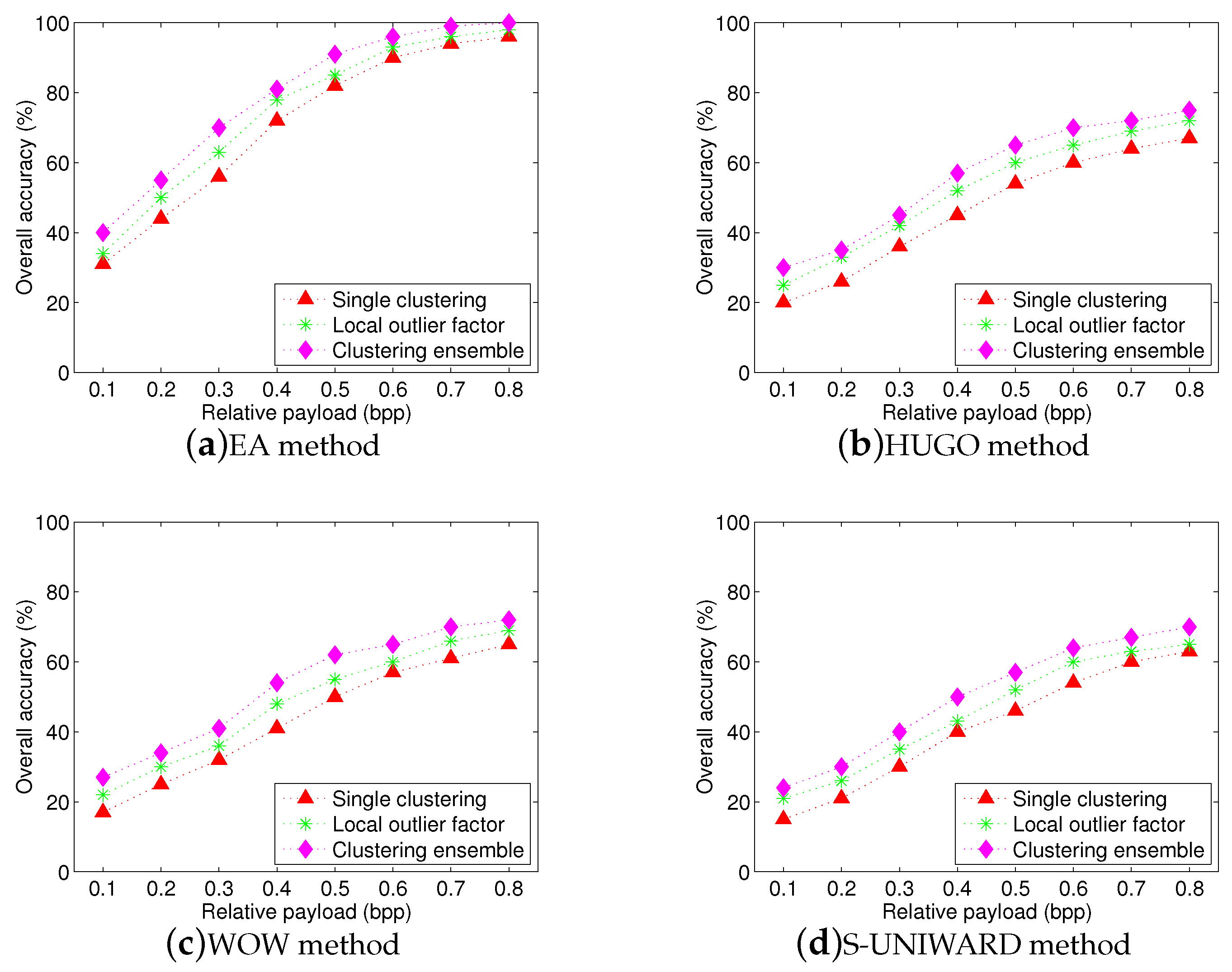
Moreover, we compare the performance of our work with single hierarchical clustering [14] and local outlier factor (LOF) [15,16] by a series of experiments. The mentioned two methods study the steganographer detection problem, while our method mainly focuses on steganographic image detection. Therefore, we adjust the experiments slightly to build a fair comparison. The cropped size is uniformly fixed = , and the number of sub-clustering is set to for single hierarchical clustering method, while (This parameter will be discussed below) for proposed clustering ensemble method. Meanwhile, we set the LOF parameter for the nearest neighbors and consider the image of the top rank as the steganographic image. SPAM-686 features and the proposed textural features are used in these methods. Here, we choose the SPAM feature set for comparison, because it is a state-of-the-art spatial steganalysis feature set and has a lower dimension, while the high-dimensional rich model feature sets are unsuitable for multi-source stego detection, for example, the maxSRM and maxSRMd2 features in Figure 5. Figure 7 and Figure 8 show the overall identification accuracy for SPAM-686 feature set and the proposed textural feature set, respectively. It can be seen that single clustering and LOF methods give an inferior performance. In addition, by comparing Figure 7 and Figure 8, we can find that the accuracies of SPAM-686 feature set are lower than that of proposed textural feature set. Overall, clustering ensemble method consistently provides a superior performance than other two methods, whatever the feature set is used. The average gains are more than and , respectively.
We also test the impact of the number of sub-clustering in the clustering ensemble step. Table 2 shows the overall identification accuracy and running time when the number of sub-clustering L is set to , respectively. In this experiment, two payloads, and , are tested. In general, the more the number of sub-clustering, the higher the overall identification accuracy, but the longer the running time. As shown from the results, no matter which payload is chosen, the overall accuracy increases slowly with an increasing L, but does not change clearly when . This is because the cropped images have a lot of overlapped areas when the number of sub-clustering increases. In this case, the diversity is reduced so that multiple clustering may generate same results. Also, we can see that the accuracy is the highest when . The running time, however, is also the longest.
4.3.3. Test for Zero or One Stego Images
In this subsection, we make the detection problem harder, by removing the assumption that exactly one image is stego. This case is rather general in real world, because we do not know whether there are any steganographic images in batch images. Therefore, we assume that either no steganographic image, or exactly one steganographic image (we leave the case that more than one guilty images to future work). In this case, we need to adjust the processing of Step 4 in Section 3.3. In Section 3.3, the last remaining image is considered to be the suspicious image. We, however, need further to decide whether or not this image is actually a stego image.
Our idea is to consider the distance between final agglomeration and penultimate agglomeration (i.e., the second to last agglomeration). If the MMD distance of final agglomeration is at least twice the MMD distance of penultimate agglomeration, then we accuse the final image as the steganographic image, otherwise, we state that no image is guilty. It is similar to deciding whether the MMD distance of the majority to the final image is at least as much as the MMD distance between any two other images, although the condition is rather strict in real world.
We implement a series of experiments to show the performance of proposed scheme for this case. The same image sources are used as in the previous experiments. We randomly select no more than 20 images, each image is cropped 50 times. The centroid clustering with Gaussian MMD is used. We measure the performance with false positives (cover is accused as stego) and false negatives (stego is considered as cover) separately from incorrect accusations (when one image is stego, but the wrong one is accused). The experiments are repeated for 100, 75, 50 times, respectively. The EA and HUGO steganographic algorithms are employed in these experiments, respectively. The corresponding results are shown in Table 3 and Table 4. We can see that there are low false positives and low incorrect accusations (even close to zero) but high false negatives for two steganographic algorithms. These experimental results indicate that the proposed scheme is conservative, because it makes a rather low false positive but often fails to accuse a steganographic image. We believe that the proposed scheme is a good start for social network steganalysis, since real-world steganalysis should be required to at least have a low false positive [36]. Figure 9 shows the overall accuracies for four steganographic algorithms. As shown in this figure, although we do not know in advance if there is a steganographic image in multiple images, the proposed scheme still achieve high overall accuracies at high relative payloads.
4.4. Comparison with the State of the Arts
4.4.1. Comparison with the Two-Step Procedure
In this subsection, we compare the proposed stego detection scheme with the naïve two-step procedure, which is also illustrated as “steganographer detection + traditional stego detection”. The two-step procedure first uses steganographer detection to find potential steganographers and then applies traditional stego detection methods, such as supervised classification, to discover steganographic images. Note that the direct comparison is rather hard, because most traditional stego detection schemes need to train a model with labelled samples, whereas our proposed scheme is unsupervised.
We build a fair comparison between the proposed scheme and the two-step procedure by adjusting the experiment as follows. All experiments are implemented in the image database including seven actors. Each actor respectively provides 600 images. We randomly select one actor as steganographer and randomly select 100 images from this actor as testing set. Among the 100 testing images, we randomly select 50 images as stego by embedding messages of relative payloads bpp using the aforementioned steganographic algorithms. The experiments are repeated 100 times. In addition,
- for the proposed scheme, we randomly select seven images, each from the seven actors, respectively. Among the seven images, one image is randomly chosen from the testing set, which includes 50 cover images and 50 stego images. The proposed scheme is run to detect this image whenever it is a stego image.
- For the two-step procedure, the training set is built by two forms as follows: excluding the testing image set (100 images), we randomly select remaining X (X = 100 and 500) images from the steganographer and then add them into the training dataset. After that, we make a copy of each image in the training dataset and embed messages in the copied image using aforementioned steganographic algorithms. Therefore, the training dataset includes images in total, which is used to train the classification model. The two-step procedure first identifies the steganographer by using steganographer detection method [17], and then uses the trained model to classify the testing set.
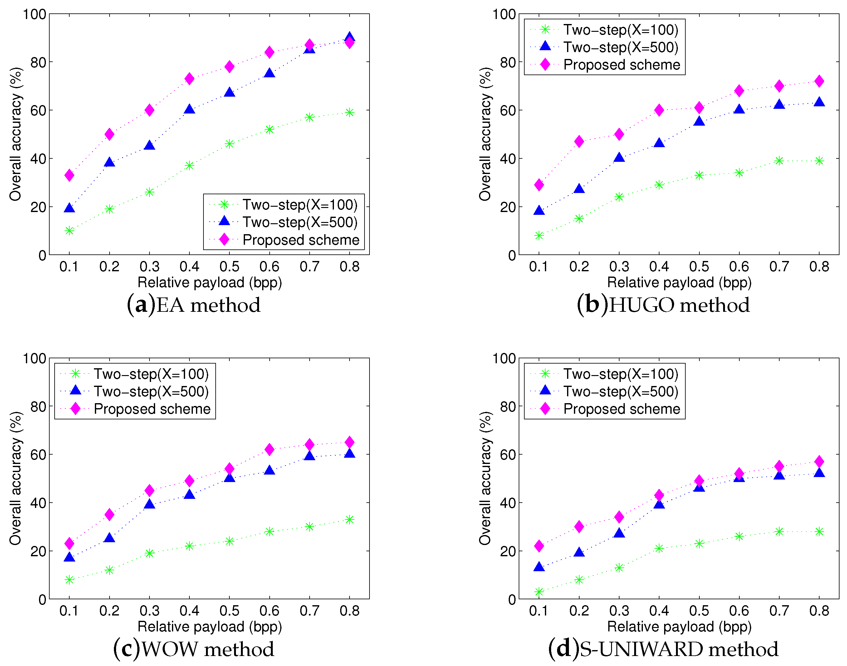
We carry out a series of experiments to compare the proposed scheme and two-step procedure (including and 500). Table 5 and Table 6 show the results of average false positives and average false negatives for the three schemes. To obtain a fair comparison, we only show the results when the steganographer is accused correctly. From these two tables, we can see that the proposed scheme has low false positives. Certainly, the proposed scheme is conservative due to high false negatives. Furthermore, when , two-step procedure has an inferior detection performance. This is because there are only a few training samples, in this case, the trained classification model may match poorly the statistic features of testing images. When , the performance of two-step procedure is significantly improved due to involving more training samples. Nevertheless, we would like to stress that it is infeasible to gather massive training samples in real-world online social media networks. Thus, the two-step procedure is very hard, at least inconvenient, to work in our context.
Figure 10 shows the overall accuracies for three schemes with four steganographic algorithms. Since the two-step procedure includes steganographer detection and traditional stego detection, when the steganographer has an incorrect identification, the accusations will be wrong directly in our experiments. We can observe that the proposed scheme achieves high overall accuracy with high relative payloads, although overall accuracy slightly decreases compared to Figure 9. Since experimental images are from multiple sources, they have different statistic distributions so that the proposed textural features extracted from these images can be influenced easily. Moreover, we can also observe that although the performance of two-step procedure has a substantial improvement with the samples increasing, its overall performance is still worse than that of proposed scheme. Two reasons can explain this phenomenon: (1) the maximum scale of training set can be up to 1000 images, but it is still small so that the trained model may not match well the statistic features of test images. Actually, this problem is inevitable because it is very hard to obtain a lot of images from the same source in social networks, (2) the accuracy will be set to zero if the steganographer has an incorrect identification at the first step of the two-step procedure. This results in a lower overall accuracy.
4.4.2. Comparison with Existing Unsupervised Method
In this section, we compare the proposed scheme with another existing unsupervised method (ATS for short) [37] that combines artificial training sets and supervised classification. ATS scheme can remove the need of a training set if there is a large enough testing set. Due to the unique design, ATS scheme is considered to bypass the cover source mismatch problem.
Since proposed scheme is an unsupervised scheme and can also potentially get around the problem of source-mismatch, we try to compare it with the ATS scheme. In order to give a fair comparison, the entire image database mentioned in Section 4.1.1, containing 4636 experimental images, is used in our experiments. Since both proposed scheme and ATS scheme have the advantage of handling data of great diversity and do not require a large number of samples to train classification model, we randomly select 500 images from entire image database as testing set. Aiming at the composition of testing set, two cases are considered: (1) Including the same number of covers and stegos, that is, 250 images are embedded secret information as stegos and another 250 as covers. (2) Including an unbalanced number of covers and stegos, that is, 100 images are embedded secret information as stegos and another 400 as covers. In addition, similar to the processing in Section 4.4.1, for the proposed scheme, we randomly select seven images in one test to separate the “outliers”. Among that one is from the testing set and the others are randomly chosen from the remaining 4136 images. Three relative payloads, bpp, are tested by using the aforementioned steganographic algorithms. The experiments are repeated 20 times and show an overall average detection accuracy as experimental results.
A series of experiments are performed to give a fair comparison. Table 7 and Table 8 respectively show the overall accuracies for two schemes with three state-of-the-art steganographic algorithms: HUGO [24], WOW [25], and S-UNIWARD [26]. In Table 7, it can be observed that proposed scheme presents the inferior detection accuracies than ATS scheme, no matter what steganographic algorithm is used, and the average gap ranges from to . On the contrary, in Table 8, proposed scheme has a slightly superior performance than ATS scheme. The average gain is approximate 1–3%. This interesting phenomenon can be explained as follows: since the proposed scheme is conservative (low false positive rate), it may be more prone to leave out the “outliers”. When there are more covers in the testing set, the detection accuracy maybe become higher. Moreover, we can notice the case that detection accuracy is less than for proposed scheme. This occurs because the proposed scheme directly implements the unsupervised classification on testing set and, hence, the results only depend on the ratio between the number of correct detection and the size of testing set. Therefore, the accuracy may be lower than with the number of correct detection decreasing.
Although proposed scheme is conservative and, thus, it may achieve a slightly inferior detection performance comparing with the ATS scheme, we, however, would like to raise the readers’ attention that it is still a good solution for social networks steganalysis due to the following two merits: (1) proposed scheme belongs to unsupervised scheme. Its main advantage is that with a reduced number of training samples, it can still address the stego detection problem successfully. (2) Due to the capability of quick detection, proposed scheme does not take much time so that it is more suitable for real-world applications.
5. Conclusions
In this paper, we addressed the multi-source stego detection problem and proposed a new steganographic image identification scheme with unsupervised learning approach, which is significantly different from steganographer detection and traditional stego detection. We designed a new low-dimensional textural feature set using local ternary pattern which is shown to be more sensitive to steganographic changes in texture regions of an image. Furthermore, ensemble mechanism with the majority voting strategy is introduced by integrating multiple hierarchical clustering to improve the identification performance. We compared our scheme with the two-step procedure, also called “steganographer detection + traditional stego detection". The results show proposed scheme has better performance. Since traditional steganalysis schemes usually work well only in laboratory, the work herein shows a valuable attempt for steganalysis in real-world online media networks.
In addition, we note that the proposed scheme is an unsupervised steganalysis method that circumvents the problem of model mismatch. However, this advantage should benefit from two aspects: (1) For each identification test, we randomly select a few clusters (e.g., ) to separate the “outliers”. This is helpful to decrease the influence of source model mismatch. (2) Unlike the single clustering schemes, we use repeated cropping in individual image to build a sub-image set and make an ensemble by multiple sub-clustering. The advantage of this approach is that, by pooling these sub-images from individual images together, the signal-to-noise ratio is significantly improved comparing with working on only individual image so that the source mismatch is finally bypassed.
Moreover, this scheme can analyse multiple images at once by assuming that the majority of them are covers and is therefore a special form of outlier detection. Although the proposed method has shown good performance in multi-source stego detection, its performance is subject to the size of images. In our scheme, the image size and content of cover source should be large and diverse enough so that the diversity in the randomly cropped images can be exploited in sub-clustering. Otherwise, if no sufficient statistical features in the cropped images can be used, the statistical features could become unstable in this case, and then the benefit of clustering ensemble may disappear, leading to poor detection in each sub-clustering.
In the future, we plan to carry our work forward in two directions. First, we should further relax the limitation for image source with different quality factor. Although the proposed scheme has shown good performance for the multi-source stego detection problem, its performance varies if the quality factor has a large variation. Second, the multi-source stego detection problem under the condition of non-uniform embedding in the image source will be considered as part of the future effort.
Author Contributions
Fengyong Li designed the algorithm, conducted the experiments and wrote the paper; Kui Wu analyzed the experimental results and polished the English; Xinpeng Zhang, Jingsheng Lei, and Mi Wen supervised the research work and provided helpful suggestions.
Acknowledgments
This work was supported by Natural Science Foundation of China under Grants (61602295, 61572311, 61472236), Natural Science Foundation of Shanghai (16ZR1413100) and the Cooperation Development Project of Industry, Education and Research for Smart Grid (A-0009-17-002-05).
Conflicts of Interest
The authors declare no conflict of interest
References
- Lyu, S.; Farid, H. Steganalysis using higher-order image statistics. IEEE Trans. Inf. Forensics Secur. 2006, 1, 111–119. [Google Scholar] [CrossRef]
- Fridrich, J. Feature-based steganalysis for JPEG images and its implications for future design of steganographic schemes. In Proceedings of the 6th International Workshop on Information Hiding, Toronto, ON, Canada, 23–25 May 2004; Volume 3200, pp. 67–81. [Google Scholar]
- Shi, Y.; Chen, C.; Chen, W. A markov process based approach to effective attacking JPEG steganography. In Proceedings of the 8th International Workshop on Information Hiding, Alexandria, VA, USA, 10–12 July 2006; Volume 4437, pp. 249–264. [Google Scholar]
- Li, F.; Zhang, X.; Cheng, H.; Yu, J. Digital image steganalysis based on local textural features and double dimensionality reduction. Secur. Commun. Netw. 2016, 9, 729–736. [Google Scholar] [CrossRef]
- Pevný, T.; Fridrich, J. Merging Markov and DCT features for multi-class JPEG steganalysis. In Proceedings of the SPIE, Electronic Imaging, Security, Steganography, and Watermarking of Multimedia Contents IX, San Jose, CA, USA, 9 January–1 February 2007; Volume 6505, pp. 3–14. [Google Scholar]
- Pevný, T.; Bas, P.; Fridrich, J. Steganalysis by subtractive pixel adjacency matrix. IEEE Trans. Inf. Forensics Secur. 2010, 5, 215–224. [Google Scholar] [CrossRef]
- Kodovský, J.; Fridrich, J.; Holub, V. Ensemble classifier for steganalysis of digital media. IEEE Trans. Inf. Forensics Secur. 2012, 7, 432–444. [Google Scholar] [CrossRef]
- Fridrich, J.; Kodovský, J. Rich models for steganalysis of digital images. IEEE Trans. Inf. Forensics Secur. 2012, 7, 868–882. [Google Scholar] [CrossRef]
- Holub, V.; Fridrich, J. Random projections of residuals for digital image steganalysis. IEEE Trans. Inf. Forensics Secur. 2013, 8, 1996–2006. [Google Scholar] [CrossRef]
- Shi, Y.; Sutthiwan, P.; Chen, L. Textural features for steganalysis. In Proceedings of the 14th International Workshop on Information Hiding, Berkeley, CA, USA, 15–18 May 2012; Volume 7692, pp. 63–77. [Google Scholar]
- Denemark, T.; Fridrich, J.; Holub, V. Further study on security of S-UNIWARD. In Proceedings of the SPIE, Electronic Imaging, Media Watermarking, Security, and Forensics, San Francisco, CA, USA, 2–6 February 2014; Volume 9028, p. 902805. [Google Scholar]
- Available online: http://www.flickr.com. (accessed on 7 March 2016).
- Available online: http://www.instagram.com. (accessed on 7 March 2016).
- Ker, A.; Pevný, T. A new paradigm for steganalysis via clustering. In Proceedings of the SPIE, Media Watermarking, Security, and Forensics III, San Francisco, CA, USA, 24–26 January 2011; Volume 7880, p. 78800U. [Google Scholar]
- Ker, A.; Pevný, T. Identifying a steganographer in realistic and hereogeneous data sets. In Proceedings of the SPIE, Media Watermarking, Security, and Forensics XIV, Burlingame, CA, USA, 23–25 January 2012; Volume 8303, pp. N01–N13. [Google Scholar]
- Ker, A.; Pevný, T. The steganographer is the outlier: Realistic large-scale steganalysis. IEEE Trans. Inf. Forensics Secur. 2014, 9, 1424–1435. [Google Scholar] [CrossRef]
- Li, F.; Wu, K.; Lei, J.; Wen, M.; Bi, Z.; Gu, C. Steganalysis over large-scale social networks with high-order joint features and clustering ensembles. IEEE Trans. Inf. Forensics Secur. 2016, 11, 344–357. [Google Scholar]
- Zhang, T.; Ping, X. A fast and effective steganalytic technique against Jsteg-like algorithm. In Proceedings of the ACM Symposium on Applied Computing, New York, NY, USA, 9–12 March 2003; pp. 307–311. [Google Scholar]
- Böhme, R. Weighted stego-image steganalysis for JPEG covers. In Proceedings of the 10th International Workshop on Information Hiding, Barbara, CA, USA, 19–21 May 2007; Volume 5284, pp. 178–194. [Google Scholar]
- Kodovský, J.; Fridrich, J. Quantitative structural steganalysis of Jsteg. IEEE Trans. Inf. Forensics Secur. 2010, 5, 681–693. [Google Scholar] [CrossRef]
- JSteg Algorithm. Available online: http://zooid.org/%7epaul/crypto/jsteg/ (accessed on 16 May 2011).
- Westfeld, A.; Pfitzmann, A. Attacks on steganographic systems. In Proceedings of the 3th International Workshop on Information Hiding, Dresden, Germany, 29 September–1 October 1999; Volume 1768, pp. 61–67. [Google Scholar]
- Luo, W.; Huang, F.; Huang, J. Edge adaptive image steganography based on LSB matching revisited. IEEE Trans. Inf. Forensics Secur. 2010, 5, 201–214. [Google Scholar]
- Pevný, T.; Filler, T.; Bas, P. Using high-dimensional image models to perform highly undetectable steganography. In Proceedings of the 12th International Workshop on Information Hiding, Calgary, AB, Canada, 28–30 June 2010; Volume 6387, pp. 161–177. [Google Scholar]
- Holub, V.; Fridrich, J. Designing steganographic distortion using directional filters. In Proceedings of the 4th International Workshop on Information Forensics and Security, Tenerife, France, 2–5 December 2012; pp. 234–239. [Google Scholar]
- Holub, V.; Fridrich, J.; Denemark, T. Universal distortion function for steganography in an arbitrary domain. EURASIP J. Inf. Secur. 2014, 1, 1–16. [Google Scholar] [CrossRef]
- Qiao, T.; Retraint, F.; Cogranne, R.; Zitzmann, C. Steganalysis of JSteg algorithm using hypothesis testing theory. EURASIP J. Inf. Secur. 2015, 2, 1–16. [Google Scholar] [CrossRef]
- Thai, T.; Cogranne, R.; Retraint, F. Statistical model of quantized DCT coefficients: Application in the steganalysis of Jsteg algorithm. IEEE Trans. Image Process. 2014, 23, 1980–1993. [Google Scholar] [CrossRef] [PubMed]
- Cogranne, R.; Zitzmann, C.; Retraint, F.; Nikiforov, I.; Cornu, P.; Fillatre, L. A local adaptive model of natural images for almost optimal detection of hidden data. Signal Process. 2014, 100, 169–185. [Google Scholar] [CrossRef]
- Gretton, A.; Borgwardt, K.; Rasch, M.; Scholkopf, B.; Smola, A. A kernel method for the two-sample-problem. In Advances in Neural Information Processing Systems 19; MIT Press: Cambridge, MA, USA, 2007; pp. 513–520. [Google Scholar]
- Huffman, D. A method for the construction of minimum redundancy codes. Proc. IRE 1952, 40, 1098–1101. [Google Scholar] [CrossRef]
- BOSSBase. Available online: http://agents.fel.cvut.cz/boss/ (accessed on 16 March 2016).
- Chang, C.; Lin, C. LIBSVM: A Library for Support Vector Machines, 2001. Software. Available online: http://www.csie.ntu.edu.tw/%7ecjlin/libsvm (accessed on 16 March 2016).
- DDE Download. Available online: http://dde.binghamton.edu/download/ (accessed on 16 March 2016).
- Denemark, T.; Sedighi, V.; Holub, V.; Cogranne, R.; Fridrich, J. Selection-channel-aware rich model for steganalysis of digital images. In Proceedings of the 6th International Workshop on Information Forensics and Security, Atlanta, GA, USA, 3–5 December 2014; pp. 48–53. [Google Scholar]
- Ker, A.; Bas, P.; Böhme, R.; Cogranne, R.; Craver, S.; Filler, T.; Fridirich, J.; Pevný, T. Moving steganography and steganalysis from the laboratory into the real world. In Proceedings of the 1st ACM Workshop on Information Hiding and Multimedia Security, Montpellier, France, 17–19 June 2013; pp. 45–58. [Google Scholar]
- Lerch-Hostalot, D.; Megías, D. Unsupervised steganalysis based on artificial training sets. Eng. Appl. Artif. Intell. 2016, 50, 45–59. [Google Scholar] [CrossRef]
Figure 1.
Framework of proposed steganalytic scheme.

Figure 2.
Different filtering processes: (a) 3 × 3 average filtering template and (b) 3 × 3 law’s mask.
Figure 2.
Different filtering processes: (a) 3 × 3 average filtering template and (b) 3 × 3 law’s mask.
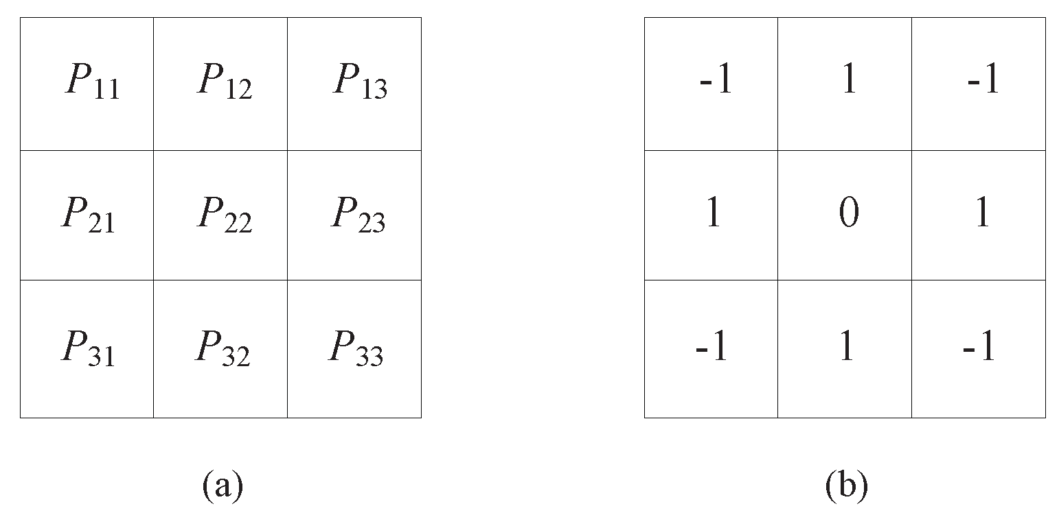
Figure 3.
Average testing error for different parameters d. The dimensions of testing features are . The classifier is G-SVM classifier and steganographic algorithms are (a) EA method and (b) HUGO method.
Figure 3.
Average testing error for different parameters d. The dimensions of testing features are . The classifier is G-SVM classifier and steganographic algorithms are (a) EA method and (b) HUGO method.

Figure 4.
The overall identification accuracy for four steganographic algorithms: (a) EA method; (b) HUGO method; (c) WOW method; and (d) S-UNIWARD method. Different cropped sizes are tested.
Figure 4.
The overall identification accuracy for four steganographic algorithms: (a) EA method; (b) HUGO method; (c) WOW method; and (d) S-UNIWARD method. Different cropped sizes are tested.
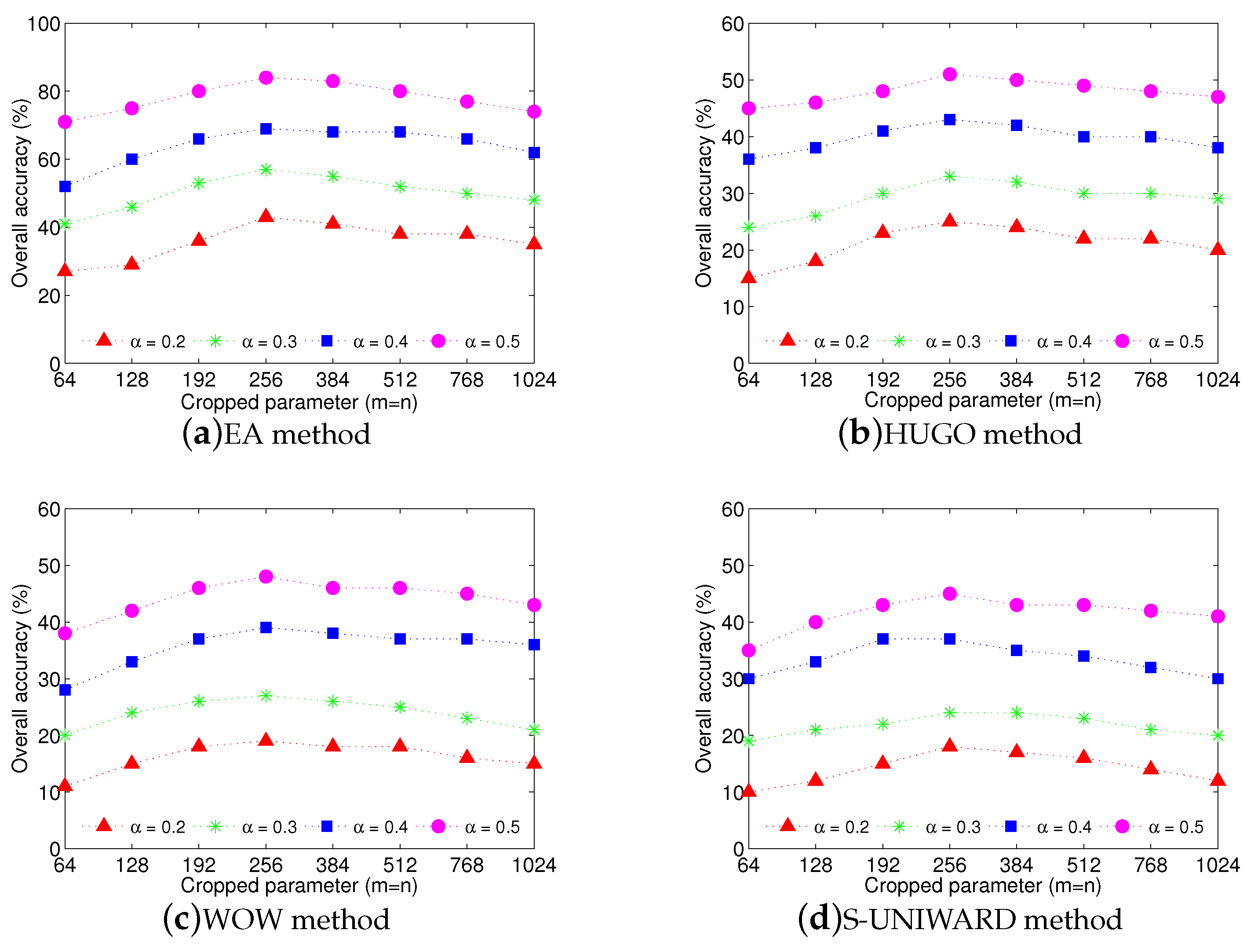
Figure 5.
Performance comparisons of four feature sets - SPAM features, maxSRM features, maxSRMd2 features and proposed textural features for (a) EA method; (b) HUGO method; (c) WOW method; and (d) S-UNIWARD method. Unsupervised clustering ensemble scheme is used in these experiments.
Figure 5.
Performance comparisons of four feature sets - SPAM features, maxSRM features, maxSRMd2 features and proposed textural features for (a) EA method; (b) HUGO method; (c) WOW method; and (d) S-UNIWARD method. Unsupervised clustering ensemble scheme is used in these experiments.

Figure 6.
Performance comparisons of four feature sets - SPAM features, maxSRM features, maxSRMd2 features and proposed textural features for (a) EA method; (b) HUGO method; (c) WOW method; and (d) S-UNIWARD method. Supervised FLD-ensemble scheme is used in these experiments.
Figure 6.
Performance comparisons of four feature sets - SPAM features, maxSRM features, maxSRMd2 features and proposed textural features for (a) EA method; (b) HUGO method; (c) WOW method; and (d) S-UNIWARD method. Supervised FLD-ensemble scheme is used in these experiments.
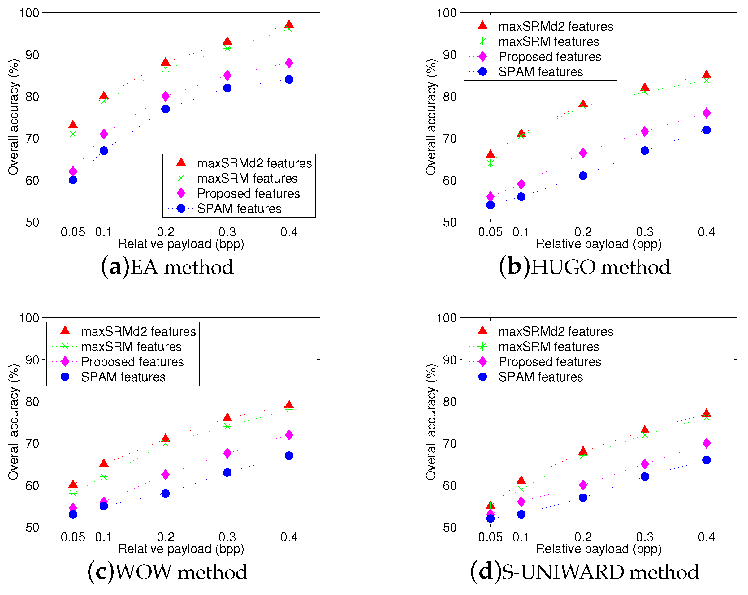
Figure 7.
Comparison of the overall identification accuracy for four steganographic algorithms: (a) EA method; (b) HUGO method; (c) WOW method; and (d) S-UNIWARD method. The steganalysis feature set is 686-dimensional SPAM feature set.
Figure 7.
Comparison of the overall identification accuracy for four steganographic algorithms: (a) EA method; (b) HUGO method; (c) WOW method; and (d) S-UNIWARD method. The steganalysis feature set is 686-dimensional SPAM feature set.

Figure 8.
Comparison of the overall identification accuracy for four steganographic algorithms: (a) EA method; (b) HUGO method; (c) WOW method; and (d) S-UNIWARD method. The steganalysis feature set is proposed 448-dimensional textural feature set.
Figure 8.
Comparison of the overall identification accuracy for four steganographic algorithms: (a) EA method; (b) HUGO method; (c) WOW method; and (d) S-UNIWARD method. The steganalysis feature set is proposed 448-dimensional textural feature set.

Figure 9.
Comparison of the overall identification accuracy for four steganographic algorithms: (a) EA method; (b) HUGO method; (c) WOW method; and (d) S-UNIWARD method, when identifying zero or one guilty images. The steganalysis feature set is proposed 448-dimensional textural feature set.
Figure 9.
Comparison of the overall identification accuracy for four steganographic algorithms: (a) EA method; (b) HUGO method; (c) WOW method; and (d) S-UNIWARD method, when identifying zero or one guilty images. The steganalysis feature set is proposed 448-dimensional textural feature set.

Figure 10.
Comparison of the overall identification accuracy between the two-step procedure (X = 100 and X = 500) and our proposed scheme. Steganographic algorithms are respectively (a) EA method; (b) HUGO method; (c) WOW method; and (d) S-UNIWARD method.
Figure 10.
Comparison of the overall identification accuracy between the two-step procedure (X = 100 and X = 500) and our proposed scheme. Steganographic algorithms are respectively (a) EA method; (b) HUGO method; (c) WOW method; and (d) S-UNIWARD method.


Table 1.
Camera model with different native resolution and quantity.
| Camera Model | Native Resolution | Quantity |
|---|---|---|
| Canon EOS M2 | 612 | |
| Nikon D90 | 643 | |
| Canon G10 | 608 | |
| Nikon D60 | 676 | |
| Canon EOS 7D | 680 | |
| Canon EOS 550D | 702 | |
| Fujifilm X-E2 | 715 |
Table 2.
Comparison of the overall identification accuracy (AR) and running time for different rounds of sub-clustering. The steganographic algorithm is EA with and bpp, respectively. The feature set is 686-dim SPAM [6,34].
| m × n | L | α = 0.4 | α = 0.6 | ||
|---|---|---|---|---|---|
| AR | Time (s) | AR | Time (s) | ||
| 5 | 52% | 4.3 | 72% | 4.4 | |
| 10 | 55% | 5.2 | 76% | 5.5 | |
| 15 | 57% | 5.7 | 79% | 6.8 | |
| 20 | 57% | 7.2 | 80% | 7.1 | |
| 25 | 58% | 8.4 | 80% | 8.3 | |
| 5 | 55% | 4.2 | 77% | 4.1 | |
| 10 | 58% | 5.3 | 80% | 5.1 | |
| 15 | 60% | 6.2 | 83% | 6.5 | |
| 20 | 60% | 7.2 | 83% | 7.4 | |
| 25 | 60% | 8.2 | 84% | 8.0 | |
| 5 | 53% | 4.9 | 75% | 4.2 | |
| 10 | 54% | 5.8 | 78% | 5.6 | |
| 15 | 57% | 6.8 | 80% | 6.6 | |
| 20 | 58% | 7.0 | 80% | 7.2 | |
| 25 | 58% | 8.3 | 81% | 8.1 | |
♯ LENOVO machine with 16 GB RAM and Intel E5-2603 Six-Core 1.60 GHz.
Table 3.
False positive (FP), false negative (FN), and incorrect accusation rate(IAR) when identifying zero or one steganographic image in five payloads (bpp). Clustering with Gaussian MMD is used and EA is targeted algorithm.
Table 3.
False positive (FP), false negative (FN), and incorrect accusation rate(IAR) when identifying zero or one steganographic image in five payloads (bpp). Clustering with Gaussian MMD is used and EA is targeted algorithm.
| Repeat | Pattern | 0.20 | 0.30 | 0.40 | 0.50 | 0.60 |
|---|---|---|---|---|---|---|
| 100 | FP | 7.0% | 6.0% | 3.0% | 2.0% | 0.0% |
| FN | 92.0% | 72.0% | 44.0% | 19.0% | 8.0% | |
| IAR | 6.0% | 4.0% | 3.0% | 1.0% | 0.0% | |
| 75 | FP | 9.3% | 6.7% | 4.0% | 1.3% | 0.0% |
| FN | 86.7% | 70.7% | 37.3% | 16.0% | 9.3% | |
| IAR | 5.3% | 4.0% | 2.7% | 0.0% | 0.0% | |
| 50 | FP | 12.0% | 8.0% | 6.0% | 2.0% | 0.0% |
| FN | 90.0% | 74.0% | 44.0% | 20.0% | 8.0% | |
| IAR | 4.0% | 2.0% | 2.0% | 0.0% | 0.0% |
Table 4.
False positive (FP), false negative (FN), and incorrect accusation rate(IAR) when identifying zero or one steganographic image in five payloads (bpp). Clustering with Gaussian MMD is used and HUGO is targeted algorithm.
Table 4.
False positive (FP), false negative (FN), and incorrect accusation rate(IAR) when identifying zero or one steganographic image in five payloads (bpp). Clustering with Gaussian MMD is used and HUGO is targeted algorithm.
| Repeat | Pattern | 0.20 | 0.30 | 0.40 | 0.50 | 0.60 |
|---|---|---|---|---|---|---|
| 100 | FP | 27.0% | 22.0% | 16.0% | 11.0% | 8.0% |
| FN | 93.0% | 88.0% | 78.0% | 61.0% | 59.0% | |
| IAR | 7.0% | 6.0% | 3.0% | 2.0% | 0.0% | |
| 75 | FP | 26.7% | 22.7% | 16.0% | 10.7% | 8.0% |
| FN | 97.3% | 90.7% | 82.7% | 75.3% | 58.0% | |
| IAR | 14.7% | 8.0% | 2.7% | 1.3% | 0.0% | |
| 50 | FP | 32.0% | 24.0% | 16.0% | 12.0% | 10.0% |
| FN | 98.0% | 90.0% | 80.0% | 76.0% | 62.0% | |
| IAR | 12.0% | 8.0% | 6.0% | 2.0% | 0.0% |
Table 5.
Average false positive (FP) and average false negative (FN) for three schemes in five payloads (bpp) when identifying zero or one steganographic image. Gaussian MMD is used in clustering, and targeted steganographic algorithm is EA.
Table 5.
Average false positive (FP) and average false negative (FN) for three schemes in five payloads (bpp) when identifying zero or one steganographic image. Gaussian MMD is used in clustering, and targeted steganographic algorithm is EA.
| Scheme | Pattern | 0.20 | 0.30 | 0.40 | 0.50 | 0.60 |
|---|---|---|---|---|---|---|
| Two-step procedure | FP | 66.3% | 61.4% | 48.7% | 37.2% | 28.5% |
| X = 100 | FN | 69.4% | 62.5% | 54.1% | 39.2% | 28.8% |
| Two-step procedure | FP | 52.4% | 44.2% | 35.7% | 29.6% | 22.5% |
| X = 500 | FN | 54.1% | 46.7% | 38.8% | 27.0% | 23.6% |
| Proposed scheme | FP | 11.6% | 9.4% | 7.8% | 5.0% | 3.8% |
| FN | 88.4% | 70.2% | 52.2% | 41.8% | 30.9% |
Table 6.
Average false positive (FP) and average false negative (FN) for three schemes in five payloads (bpp) when identifying zero or one steganographic image. Gaussian MMD is used in clustering, and targeted steganographic algorithm is HUGO.
Table 6.
Average false positive (FP) and average false negative (FN) for three schemes in five payloads (bpp) when identifying zero or one steganographic image. Gaussian MMD is used in clustering, and targeted steganographic algorithm is HUGO.
| Scheme | Pattern | 0.20 | 0.30 | 0.40 | 0.50 | 0.60 |
|---|---|---|---|---|---|---|
| Two-step procedure | FP | 85.3% | 78.5% | 72.1% | 66.3% | 62.5% |
| X = 100 | FN | 86.2% | 78.6% | 70.9% | 65.6% | 60.6% |
| Two-step procedure | FP | 74.5% | 61.4% | 58.1% | 45.3% | 40.8% |
| X = 500 | FN | 76.4% | 62.7% | 56.9% | 47.8% | 40.2% |
| Proposed scheme | FP | 19.8% | 16.0% | 11.8% | 9.2% | 6.8% |
| FN | 90.6% | 88.8% | 74.6% | 70.2% | 63.6% |
Table 7.
Average detection accuracy (%) for proposed schemes and ATS scheme [37] in three payloads (bpp). The testing set includes the same number of covers and stegos. The targeted steganographic algorithms are HUGO, WOW, and S-UNIWARD.
Table 7.
Average detection accuracy (%) for proposed schemes and ATS scheme [37] in three payloads (bpp). The testing set includes the same number of covers and stegos. The targeted steganographic algorithms are HUGO, WOW, and S-UNIWARD.
| Steganographic Algorithm | Scheme | Payloads | ||
|---|---|---|---|---|
| 0.20 | 0.40 | 0.60 | ||
| HUGO | ATS Scheme | 55.4% | 61.2% | 70.4% |
| Proposed Scheme | 47.6% | 55.8% | 67.7% | |
| WOW | ATS Scheme | 53.1% | 58.4% | 66.8% |
| Proposed Scheme | 42.6% | 51.2% | 60.8% | |
| S-UNIWARD | ATS Scheme | 51.5% | 55.8% | 62.2% |
| Proposed Scheme | 40.6% | 46.6% | 55.2% | |
Table 8.
Average detection accuracy (%) for proposed schemes and ATS scheme [37] in three payloads (bpp). The testing set includes an unbalanced number of covers and stegos. The targeted steganographic algorithms are HUGO, WOW, and S-UNIWARD.
Table 8.
Average detection accuracy (%) for proposed schemes and ATS scheme [37] in three payloads (bpp). The testing set includes an unbalanced number of covers and stegos. The targeted steganographic algorithms are HUGO, WOW, and S-UNIWARD.
| Steganographic Algorithm | Scheme | Payloads | ||
|---|---|---|---|---|
| 0.20 | 0.40 | 0.60 | ||
| HUGO | ATS Scheme | 57.4% | 66.2% | 75.4% |
| Proposed Scheme | 60.6% | 66.8% | 77.7% | |
| WOW | ATS Scheme | 55.1% | 64.4% | 73.8% |
| Proposed Scheme | 57.6% | 67.2% | 74.1% | |
| S-UNIWARD | ATS Scheme | 54.5% | 63.8% | 70.2% |
| Proposed Scheme | 58.6% | 65.6% | 71.2% | |
© 2018 by the authors. Licensee MDPI, Basel, Switzerland. This article is an open access article distributed under the terms and conditions of the Creative Commons Attribution (CC BY) license (http://creativecommons.org/licenses/by/4.0/).
Share and Cite
MDPI and ACS Style
Li, F.; Wu, K.; Zhang, X.; Lei, J.; Wen, M. Multi-Source Stego Detection with Low-Dimensional Textural Feature and Clustering Ensembles. Symmetry 2018, 10, 128. https://doi.org/10.3390/sym10050128
AMA Style
Li F, Wu K, Zhang X, Lei J, Wen M. Multi-Source Stego Detection with Low-Dimensional Textural Feature and Clustering Ensembles. Symmetry. 2018; 10(5):128. https://doi.org/10.3390/sym10050128
Chicago/Turabian StyleLi, Fengyong, Kui Wu, Xinpeng Zhang, Jingsheng Lei, and Mi Wen. 2018. "Multi-Source Stego Detection with Low-Dimensional Textural Feature and Clustering Ensembles" Symmetry 10, no. 5: 128. https://doi.org/10.3390/sym10050128
Note that from the first issue of 2016, this journal uses article numbers instead of page numbers. See further details here.