Article

Feedforward Neural Networks with a Hidden Layer Regularization Method

School of Mathematical Sciences, Dalian University of Technology, Dalian 116024, China
*
Author to whom correspondence should be addressed.
Symmetry 2018, 10(10), 525; https://doi.org/10.3390/sym10100525
Submission received: 3 September 2018 / Revised: 13 October 2018 / Accepted: 14 October 2018 / Published: 19 October 2018

Abstract

:
In this paper, we propose a group Lasso regularization term as a hidden layer regularization method for feedforward neural networks. Adding a group Lasso regularization term into the standard error function as a hidden layer regularization term is a fruitful approach to eliminate the redundant or unnecessary hidden layer neurons from the feedforward neural network structure. As a comparison, a popular Lasso regularization method is introduced into standard error function of the network. Our novel hidden layer regularization method can force a group of outgoing weights to become smaller during the training process and can eventually be removed after the training process. This means it can simplify the neural network structure and it minimizes the computational cost. Numerical simulations are provided by using K-fold cross-validation method with K = 5 to avoid overtraining and to select the best learning parameters. The numerical results show that our proposed hidden layer regularization method prunes more redundant hidden layer neurons consistently for each benchmark dataset without loss of accuracy. In contrast, the existing Lasso regularization method prunes only the redundant weights of the network, but it cannot prune any redundant hidden layer neurons.

1. Introduction

Artificial Neural Networks (ANNs) are pretty old ideas to mimic the human brain [1]. ANNs have been intensively studied for many years in the hope of achieving human-like performance in the fields of speech and image recognition [2]. They are designed to solve a variety of problems in the area of pattern recognition, prediction, optimization, associative memory, and control [3]. ANNs are also used for approximation of phenol concentration using computational intelligence methods [4].
The Feedforward Neural Networks (FNNs) are the most fundamental part of ANNs that have been trained by using the connectionist learning procedure called a supervised manner which requires a teacher to specify the desired output vector [5]. An FNN is one part of a multi-layer perceptron (MLP) with unidirectional data flow [6]. In FNNs, the neurons are arranged in the form of layers, namely input, hidden and output layers and there exist the connections between the neurons of one layer to those of the next layer [7]. These connections are repeatedly adjusted to minimize a measure of the difference between the actual network output vector and the desired output vector through the learning process [8]. The FNNs are commonly trained by using the backpropagation (BP) algorithm which uses a gradient descent learning method, also called the steepest descent [9].
Depending on the way the weights are updating, the gradient descent method can be classified into the following three methods: batch gradient descent method, mini-batch gradient descent method and stochastic gradient descent method. In the batch gradient descent method, the weights are updated after all the training examples are shown to the learning algorithm. In the stochastic gradient descent method, the weight parameters are updated using each training example. In a mini-batch gradient descent method, the training examples are partitioned into small batches, and the weight parameters are updated for each mini-batch example. In this study, we focus only on the batch gradient method.
It is well known that determining the number of input and output neurons naturally depends on the dimension of the problem, but the main problem is determining the optimal number of neurons in the hidden layer that can solve the specific problem [10]. Here, we mean the optimal number of the hidden layer neurons of FNNs is one that is large enough to learn the samples and small enough to perform well on unseen samples. There is no clear standard method to determine the optimal size of the hidden layer neurons for the network to solve a specific problem. However, usually, the number of hidden neurons of the neural network is determined by a trial-and-error method. This will lead to a cost problem in computation. In addition, having too many neurons in the hidden layer may lead to overfitting of the data and poor generalization while having too few neurons in the hidden layer may not provide a network that learns the data [11].
Generally speaking, the constructive and destructive approaches are the two main approaches used in literature for optimizing neural network structure [12]. The first approach, also called the growing method, begins with a minimal neural network structure and adds more hidden neurons only when they are needed to improve the learning capability of the network. The second approach begins with an oversized neural network structure and then prunes redundant hidden layer neurons [13]. A disadvantage of applying the growing method is that the initial neural network with a small number of hidden layer neurons can easily be trapped into local minima and it may need more time to get the optimal number of hidden layer neurons. Therefore, we aimed to find the optimal number of hidden layer neurons by using the pruning method.
Furthermore, depending on the techniques used for pruning, the pruning methods can be further classified into the following methods [14]: regularization (penalty) methods, cross-validation methods, magnitude base methods, evolutionary pruning methods, mutual information, significance based pruning methods, and the sensitivity analysis method. The most popular sensitivity based pruning algorithms are the Optimal Brain Damage [15] and the Optimal Brain Surgeon method [16]. This paper focuses on a pruning technique called the regularization method that mainly addresses the overfitting problem. To do this, we can add the extra regularization terms into the standard error function to sparse the values of weight connections by assuming that sparse neural network models lead to better performance.
Most of the existing regularization methods for FNNs can be further categorized into different L p regularization methods. Figure 1 indicates a graphical representation of L p norms with different p-values.
The L p regularization method is widely applied as a parameter estimation technique to solve the variable selection problem [17]. The most common L p regularization terms are
R ( W ) = 1 2 i W w i 2 , L 2 regularization ,
R ( W ) = i W | w i | , L 1 regularization ,
R ( W ) = i W | w i | 1 / 2 , L 1 / 2 regularization ,
where W is the set of all weights of the neural network and | · | represents the absolute value function. The regularization term in Equation (1) is defined as the 2-norm (squared norm) of the network weights. L 2 regularization does not have the sparsity property, but it has the property of being smooth. The L 1 regularization term leads to an area of the convex optimization problem, which is easy to solve, but it does not give a sufficiently sparse solution [18]. Adding the L 1 / 2 regularization term into the standard error function promotes excess weights to take values close to zero. The L 1 / 2 regularization term performs better in the sparsity of weight connections [19,20,21]. Recently, the L 1 / 2 regularization term has been proposed to determine the redundant dimensions of the input data for the multilayer feedforward networks by fixing the number of hidden neurons [22]. The result of this study confirms that the L 1 / 2 regularization method produces better performance than L 1 due to its sparsity property.
To sum up, a major drawback of using the L p regularization terms described above is that they are mainly designed for removing the redundant weights from the neural network, but they cannot remove the redundant or unnecessary hidden neurons of the neural network automatically. This study aimed to investigate the pruning of unnecessary hidden layer neurons of FNNs.
The popular Lasso, least absolute shrinkage and selection operator, regularization method that was originally proposed for estimation of linear models is defined in [23] as
β ^ L a s s o ( λ ) = arg min Y X β 2 2 + λ β 1 ,
where λ is a regularization parameter, Y R m is a continuous response, X is an m × k design matrix, β R k is a vector parameter. Moreover, · 2 2 and · 1 stands for 2-norm (squared norm) and 1-norm, respectively. Lasso tends to produce sparse solutions for network models.
An extension of Lasso, group Lasso was originally used to solve linear regression problems and it is one of the most popular regularization method for variable selection [24,25]. For a given training set that consists of M input-output pairs f ( x i , y i ) 1 i M , the following optimization problem with group Lasso regularization term was used in [26] to sparse the network with any L numbers of layers that consists of N l neurons numbers each of which is encoded by parameters θ l n = [ w l n , b l n ] , w l n is a linear operator acting on the layer’s input and b l n is a bias, where these parameters form the parameter set Θ = θ l 1 l L , with θ = θ l n 1 n N l ,
min Θ 1 M i = 1 M ( y i , f ( x i , Θ ) ) + l = 1 L λ l p l n = 1 N l θ l n 2 ,
where ( . ) is a loss function that compares the network prediction with the ground-truth output, such as the logistic loss for classification or the square loss for regression, p l is the size of parameters grouped together in layer l and λ l is the regularization coefficient. The regularization parameters λ l are scaled with group size p l to regularize larger groups in (5). Here, tuning different regularization parameters λ l for each groups in each layer is considered as one disadvantage. However, by rescaling the groups, we can simplify the cost function in Equation (5) into
min Θ 1 M i = 1 M ( y i , f ( x i , Θ ) ) + λ l = 1 L n = 1 N l θ l n 2 .
Now, one can use Equation (6) that is simplified from Equation (5) to sparse the neural network structure by penalizing each group in each layer with the same regularization parameter λ . Particularly, it is important to prune the redundant neurons from the input and hidden layers.
Hence, developing an automated hidden layer regularization method by using the idea of Equation (6), which can find out a small, necessary, and sufficient number of neurons in the hidden layer of FNNs without an additional retraining process is our primary motivation. To achieve this, there are two approaches. The first approach is considering only the norm of the total entering weights to each hidden layer neurons. The second approach is considering only the norm of the total outgoing weights from each hidden layer neurons. In this paper, we propose a group Lasso regularization method by using the second approach. Here, our goal is shrinking the total outgoing weights from unnecessary or redundant neurons of the hidden layer to zero without loss of accuracy.
Furthermore, we conduct experiments by using the benchmark datasets to compare our proposed hidden layer regularization method with the standard batch gradient method without any regularization term and the popular Lasso regularization method. The numerical results demonstrate the effectiveness of our proposed hidden layer regularization method on both sparsing and generalization ability.
The rest of this paper is organized as follows: in Section 2, Materials and Methods are described. In Section 3, the results are presented. In Section 4, we discuss in detail the numerical results. Finally, we conclude this paper with some remarks in Section 5.

2. Materials and Methods

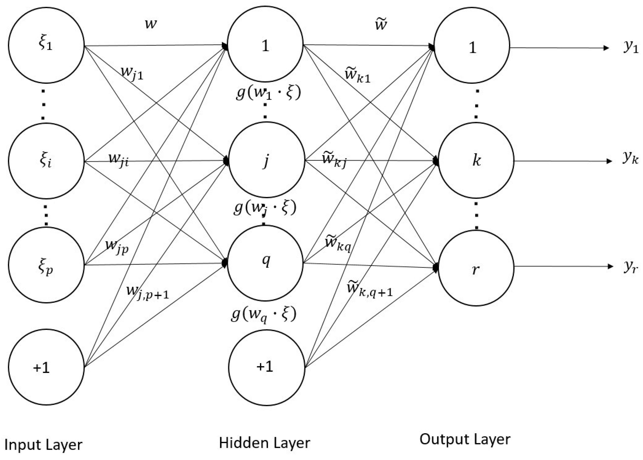
2.1. Neural Network Structure and Batch Gradient Method without Regularization Term

We consider an FNN with one hidden layer of the network structure p + 1 q + 1 r , consisting of p + 1 number of neurons in the input layer, q + 1 number of neurons in the hidden layer and r number of neurons in the output layer (including bias neurons in the input and hidden layers) (see Figure 2). Here, the extra neuron added into both input and hidden layers represents the bias neuron with output value +1, and it allows us to shift the activation function to the left or right, which is very important for successful network training process. We note that this fully connected neural network structure has q ( p + 1 ) + r ( q + 1 ) total number of weight connections. To perform computations for our given neural network structure, we represent the weight connections of the neural network in the form of matrices and vectors and apply matrix-vector operations. Let w j = ( w j 1 , w j 2 , w j 3 , , w j i , , w j p , w j ( p + 1 ) ) T R p + 1 be the weight vector connecting the input neurons and the hidden layer neuron j ( j = 1 , 2 , 3 , , q ) and w ˜ k = ( w ˜ k 1 , w ˜ k 2 , w ˜ k 3 , , w ˜ k j , , w ˜ k q , w ˜ k ( q + 1 ) ) T R q + 1 be the weight vector connecting the hidden layer neurons and the output neuron k ( k = 1 , 2 , 3 , , r ) , where the symbol “T” represents the transpose. We can also represent in matrix form as shown below:
w = ( w 1 , w 2 , w 3 , , w j , , w q ) T R q × ( p + 1 ) , w ˜ = ( w ˜ 1 , w ˜ 2 , w ˜ 3 , , w ˜ k , , w ˜ r ) T R r × ( q + 1 ) .
To make our presentation simple, we can rewrite all the weight parameters in a compact form as follows: W = ( w ˜ 1 T , w ˜ 2 T , w ˜ 3 T , , w ˜ k T , , w ˜ r T , w 1 T , w 2 T , w 3 T , , w j T , , w q T ) T R r ( q + 1 ) + q ( p + 1 ) . Let g : R R be a given activation function for hidden layer neurons and output neurons which is typically but not necessarily a sigmoid function that squashes (limits) the outputs of the summation neurons. For any x = ( x 1 , x 2 , x 3 , , x j , , x q ) T R q , we introduce the vector-valued function
G : R q R q + 1 , G ( x ) = ( g ( x 1 ) , g ( x 2 ) , g ( x 3 ) , , g ( x j ) , , g ( x q ) , + 1 ) T ,
where component + 1 represents the output value from bias neuron. Let ξ m , o m m = 1 M R P + 1 × R r be a set of training examples, where ξ m = ( ξ 1 m , ξ 2 m , ξ 3 m , , ξ i m , , ξ p m , + 1 ) T R p + 1 and o m R r are the input and the corresponding one-hot encoded ideal output of the mth sample, respectively. Then, for each input ξ m , the actual output vector of the hidden layer neurons is G ( w ξ m ) and finally the actual output to the network at output neuron k is:
y k m = g w ˜ k · G ( w ξ m ) .
Consequently, the actual output vector to the network at output layer is: y m = ( y 1 m , y 2 m , y 3 m , y k m , , y r m ) T R r .
Then, the standard mean square error function to the network without any regularization term is defined as
E ˜ ( W ) = 1 2 M m = 1 M k = 1 r o k m y k m 2 = 1 2 M m = 1 M k = 1 r o k m g w ˜ k · G ( w ξ m ) 2 = m = 1 M k = 1 r g m k w ˜ k · G ( w ξ m ) ,
where
g m k ( t ) = 1 2 M ( o k m g ( t ) ) 2
is a composite function and its derivative is
g m k ( t ) 1 M ( o k m g ( t ) ) g ( t ) , t R , m = 1 , 2 , , M .
Then,
E ˜ w ˜ k j ( W ) = m = 1 M g m k w ˜ k · G ( w ξ m ) g ( w j ξ m ) ,
E ˜ w j i ( W ) = m = 1 M k = 1 r g m k w ˜ k · G ( w ξ m ) w ˜ k j g ( w j ξ m ) ξ i m ,
for i = 1 , 2 , 3 , , p , p + 1 ; j = 1 , 2 , 3 , , q , q + 1 and k = 1 , 2 , 3 , , r . The gradient of the error function defined in Equation (9) with respect to the weight vector W is also defined as
E ˜ W ( W ) = ( E ˜ w ˜ 1 T , E ˜ w ˜ 2 T , E ˜ w ˜ 3 T , , E ˜ w ˜ k T , , E ˜ w ˜ r T , E ˜ w 1 T , E ˜ w 2 T , E ˜ w 3 T , , E ˜ w j T , , E ˜ w q T ) T R r ( q + 1 ) + q ( p + 1 ) ,
where
E ˜ w ˜ 1 T = E ˜ w ˜ 11 ( W ) , E ˜ w ˜ 12 ( W ) , E ˜ w ˜ 13 ( W ) , , E ˜ w ˜ 1 j ( W ) , , E ˜ w ˜ 1 q ( W ) , E ˜ w ˜ 1 ( q + 1 ) ( W ) , E ˜ w ˜ 2 T = E ˜ w ˜ 21 ( W ) , E ˜ w ˜ 22 ( W ) , E ˜ w ˜ 23 ( W ) , , E ˜ w ˜ 2 j ( W ) , , E ˜ w ˜ 2 q ( W ) , E ˜ w ˜ 2 ( q + 1 ) ( W ) , E ˜ w ˜ r T = E ˜ w ˜ r 1 ( W ) , E ˜ w ˜ r 2 ( W ) , E ˜ w ˜ r 3 ( W ) , E ˜ w ˜ r j ( W ) , , E ˜ w ˜ r q ( W ) , E ˜ w ˜ r ( q + 1 ) ( W ) , E ˜ w 1 T = E ˜ w 11 ( W ) , E ˜ w 12 ( W ) , E ˜ w 13 ( W ) , , E ˜ w 1 i ( W ) , , E ˜ w 1 p ( W ) , E ˜ w 1 ( p + 1 ) ( W ) , E ˜ w 2 T = E ˜ w 21 ( W ) , E ˜ w 22 ( W ) , E ˜ w 23 ( W ) , , E ˜ w 2 i ( W ) , , E ˜ w 2 p ( W ) , E ˜ w 2 ( p + 1 ) ( W ) , E ˜ w q T = E ˜ w q 1 ( W ) , E ˜ w q 2 ( W ) , E ˜ w q 3 ( W ) , , E ˜ w q i ( W ) , , E ˜ w q p ( W ) , E ˜ w q ( p + 1 ) ( W ) .

2.2. A Batch Gradient Method with Hidden Layer Regularization Terms

The network complexity is usually measured in terms of the number of free parameters, i.e., by the total number of weights in the network. By adding any regularization terms into the standard error function we can limit the growth of the weights during network training process. In the next section we construct the proposed hidden layer regularization terms that can remove unnecessary or redundant hidden layer neurons of FNNs.

2.2.1. Batch Gradient Method with Lasso Regularization Term

We first describe the popular Lasso regularization method. Here, our main concerned is to penalize each weight connections of the neural network by using the Lasso regularization term. The new error function E ( W ) with Lasso hidden layer regularization term is defined as follows:
E ( W ) = E ˜ ( W ) + λ W 1 ,
where E ˜ ( W ) is the standard error function defined in Section 2.1, W 1 = i W w i , W is the set of all weights and λ is the regularization parameter that prevents the network weights from growing too large by penalizing each weight during network training.
The goal of the network training is to get W * such that
W * = arg min E ˜ ( W ) + λ W 1 .
The gradients of the error function in Equation (12) with respect to w j i and w ˜ k j are expressed, respectively as
E w j i ( W ) = E ˜ w j i ( W ) + λ sign ( w j i ) ,
E w ˜ k j ( W ) = E ˜ w ˜ k j ( W ) + λ sign ( w ˜ k j ) ,
where the “sign” is signum function of a real number x that can be defined as follows:
sign ( x ) = 1 if x < 0 , 0 if x = 0 , 1 if x > 0 .
The corresponding increments of the weights w j i n and w ˜ k j n are respectively defined as follows:
w j i n = η E ˜ w j i n ( W ) + λ sign ( w j i n ) ,
w ˜ k j n = η E ˜ w ˜ k j n ( W ) + λ sign ( w ˜ k j n ) ,
where η is a positive parameter that controls the speed of learning process.
In the above equations, the minus sign indicates that the learning is taking place in the opposite direction to the gradient descent, which is the steepest descent. Starting with initial value W 0 , the weight vector W n is updated iteratively by using the following learning algorithm:
W n + 1 = W n + W n .
In component form, the weights are updated iteratively by
w j i n + 1 = w j i n + w j i n ,
w ˜ k j n + 1 = w ˜ k j n + w ˜ k j n .

2.2.2. Batch Gradient Method with Group Lasso Regularization Term

Now, let us formulate our proposed hidden layer regularization method. This is done by penalizing only the norm of total outgoing weights from each hidden layer neuron. Its new error function is formulated as
E ( W ) = E ˜ ( W ) + λ j = 1 q + 1 w ˜ j 2 ,
where w ˜ j 2 = w ˜ 1 j 2 + w ˜ 2 j 2 + + w ˜ k j 2 + + w ˜ r j 2 1 2 is the 2- norm (not squared norm) of outgoing weight vector from the j-th hidden layer neuron, and λ is the regularization parameter. Similarly, the goal of the network training by using group Lasso is also to get W * such that
W * = arg min E ˜ ( W ) + λ j = 1 q + 1 w ˜ j 2 .
Adding the extra group Lasso regularization term into the standard error function plays a great role to shrink all the outgoing weights of a redundant or unnecessary hidden layer neuron j of FNNs. Hence, any neuron j of a hidden layer with the norm of its outgoing weights is zero or near to zero should be automatically removed without degradation of the neural network accuracy.
The corresponding gradients of the error function defined in Equation (19) with respect to w j i and w ˜ k j are expressed, respectively, as
E w j i ( W ) = E ˜ w j i ( W ) ,
E w ˜ k j ( W ) = E ˜ w ˜ k j ( W ) + λ w ˜ k j w ˜ j 2 .
Thus,
w j i n = η E ˜ w j i n ( W ) ,
w ˜ k j n = η E ˜ w ˜ k j n ( W ) + λ w ˜ k j n w ˜ j n 2 .
By starting with initial weight vector W 0 , the weight vector W n are updated iteratively by using the learning algorithm formulated by the Equation (17). Similarly, each weight component is also updated iteratively by using Equations (18a) and (18b).

2.3. Datasets

Four benchmark datasets from the UCI machine learning repository [27] are chosen for numerical simulation purposes and their detail properties are described in Table 1.
The first dataset is an iris dataset, which is one of the well-known benchmark datasets in machine learning. It contains three sets of flower types (Iris Setosa, Iris Versicolour, and Iris Virginica) and four dimensions (sepal length in cm, sepal width in cm, petal length in cm, petal width in cm).
The second one is the zoo dataset which is one of the seven class classification datasets. It contains 101 examples, each with 17 Boolean-valued attributes. Our task is to classify animals into 7 categories based on given information.
The third dataset is the seeds dataset, which is one of the multiclass classification datasets. It contains 210 examples, each with seven features. Our task is to classify varieties of wheat into three classes (i.e., Kama, Rosa and Canadian).
The fourth dataset that we use is ionosphere dataset. This radar dataset was collected by a system in Goose Bay, Labrador. This system consists of a phased array of 16 high-frequency antennas with a total transmitted power on the order of 6.4 kilowatts. The targets were free electrons in the ionosphere. “Good” radar returns are those showing evidence of some type of structure in the ionosphere. “Bad” returns are those that do not; their signals pass through the ionosphere. This data has 351 instances and 35 attributes. All 34 predictor attributes are continuous, and the 35th attribute is either “Good” or “Bad”. This is a binary classification task.

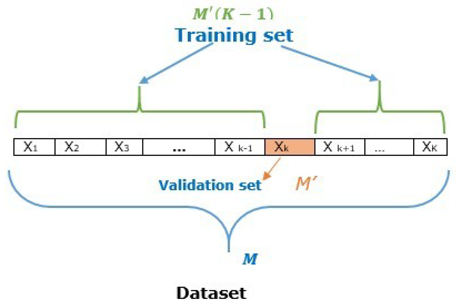
2.3.1. K-fold Cross-Validation Method

To avoid overtraining, we use the K-fold cross-validation method [28]. The parameter K represents the fold size. First, we shuffled the original dataset, X = ξ m , o m m = 1 M R P + 1 × R r , randomly. As shown in Figure 3 the shuffled dataset is divided into K roughly equal-sized sub datasets, X 1 , X 2 , X 3 , , X k , , X K , where X k = ξ m , o m m = 1 M R P + 1 × R r and M = M K is the size of each fold. One of the K sets is used as the validation set for validating the trained network while the remaining K 1 datasets are used as training set. Hence the training set, X t r a i n = X 1 , X 2 , X 3 , , X k 1 , X k + 1 , , X K and the validation set, X v a l i d a t i o n = X k .
The cross-validation process is repeated K times (K folds). The advantage of applying K-fold is that each fold is used exactly once as the validation set. Finally, the K results are averaged to obtain a single average accuracy result.
For a given set of learning parameters W , η , λ , K , we compute the training accuracy for each k = 1 , 2 , 3 , , K as follows:
T r a i n i n g A c c u r a c y ( k ) = 1 M ( K 1 ) m = 1 M ( K 1 ) I ( arg max k = 1 , 2 , , r y m , arg max k = 1 , 2 , , r o m ) ,
where, the indicative function I ( a , b ) = 1 , if a = b , 0 , if a b , and y m and o m are predicted vector of all output layer neurons and a one-hot encoded ideal output of X t r a i n , respectively. The corresponding testing accuracy is computed as
T e s t i n g A c c u r a c y ( k ) = 1 M m = 1 M I ( arg max k = 1 , 2 , , r y m , arg max k = 1 , 2 , , r o m ) .
Similarly, y m and o m are predicted vectors of all output layer neurons and a one-hot encoded ideal output of X v a l i d a t i o n . Finally, the average training and testing accuracy of all K results are computed respectively as
T r a i n i n g A c c u r a c y = 1 K k = 1 K T r a i n i n g A c c u r a c y ( k ) ,
T e s t i n g A c c u r a c y = 1 K k = 1 K T e s t i n g A c c u r a c y ( k ) .
All numerical simulations were run on a MacBook Air laptop designed by apple in California assembled in China with the processor running at 1.6 GHz Intel Core i5, Memory 8 GB 1600 NHz DDR3 and Graphics Intel HD Graphics 6000 1536 MB of RAM by using MATLAB R2014a (MathWorks, Inc., Natick, MA, USA).

2.3.2. Data Normalization

In the data mining area, data preprocessing is a crucial technique to clean the data before we are using it for the neural network training process. The normalization is needed to improve the performance of numerical computation and obtain better neural network output results by avoiding the influence of one attribute over another. A min-max normalizing method [29] is one of the most common data normalizing methods and it is defined as
z i = x i min ( x ) max ( x ) min ( x ) max n e w min n e w + min n e w ,
where x = [ x 1 , x 2 , x 3 , , x n ] T is original data values of a single feature of dataset, x i is i-th original data value and z i is i-th normalized data value. The max n e w and min n e w represent the maximum range and minimum range for normalized dataset, respectively. Thus, each of the original benchmark dataset is normalized in a range of 0 to 1. All class attributes of the benchmark dataset are also encoded by one-hot representation.

2.3.3. Activation Function

A pure linear (purelin) activation function with the range ( , ) is the most common activation function for the output layer in MATLAB. Herein, after we normalized our datasets, we choose the logistic sigmoid function as a transfer function for all neurons in the hidden layer and output layer and it is expressed as
logsig ( x ) = 1 1 + exp ( x ) .
The logistic sigmoid activation function has the range ( 0 , 1 ) . This function can work well for classification tasks by giving the output results at the output layer in the range 0 to 1.

2.4. Hidden Neuron Selection Criterion

To determine whether a neuron j in the hidden layer will survive or remove after training, the strategy that we used as a neuron selection criterion is just computing the norm of total outgoing weights from the neuron j. In literature, there is no standard threshold value to remove unnecessary weight connections and redundant neurons from the initially assumed neural network structure. According to [20,30], the sparsity of the learning algorithm was measured by using the number of weights whose absolute values are ≤0.0099 and ≤0.01, respectively. In this study, we have arbitrary chosen 0.00099 as a threshold value which is more less than the existing thresholds in literature.
Training algorithm and heuristics for FNN parameter selection
  • Use a K-fold cross-validation method to split the dataset into a training set and validation set.
  • Pick large fully connected FNNs with structure p + 1 q + 1 r , where p + 1 is neuron number in the input layer, q + 1 is neuron number in the hidden layer, and r is neuron number in the output layer (including bias neuron). The number of the input layer and output layer neurons are set equal to the numbers of attributes and classes for each dataset, respectively. Likewise, the number of hidden layer neurons initially is set randomly in a way that it needs to be remarkably bigger than the numbers of attributes and classes.
  • Randomly initialize network weights w and w ˜ in [ 0.5 , 0.5 ] .
  • For each k = 1 , 2 , 3 , , K train the network using a training set with the standard batch gradient method without any regularization term (i.e., λ = 0 ) as a function learning rate η and pick the best η that gives the best learning.
  • Use the best learning rate η obtained from step 3 and start the training process further by increasing the regularization coefficient λ up to too many numbers of hidden layer neurons are removed, and the accuracy of the network is degraded.
  • Compute the norm of the total outgoing weights from each neuron j in the hidden layer; if the norm of total outgoing weights from neuron j in the hidden layer is less or equal to the threshold value, then remove the neuron j from the network else the neuron j will survive.
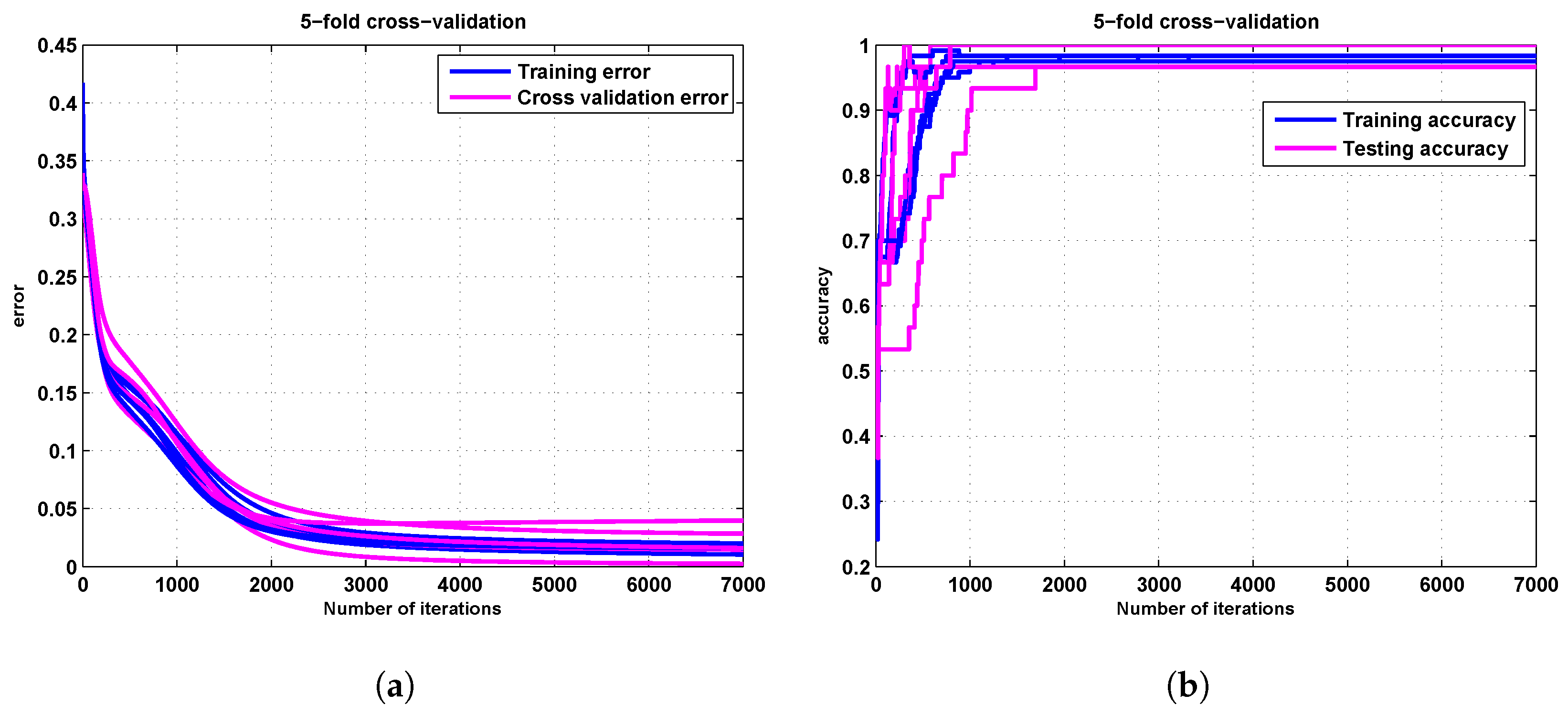
  • Compute the training accuracy using Equation (23).
  • Evaluate the trained network using a validation set.
  • Compute the testing accuracy using Equation (24).
  • Compute the average training and average testing accuracy of the overall results of K using Equations (25) and (26), respectively.
  • Compute the average number of redundant or unnecessary hidden layer neurons.
  • Select the best regularization parameter λ that gives the best average results.

3. Results

In this section, we present the numerical results of our proposed batch gradient method with a group Lasso regularization term (BGGLasso) compared to the existing learning methods (i.e., standard batch gradient method without any regularization term (BG) and batch gradient method with a Lasso regularization term (BGGLasso)) using benchmark datasets. Accuracy and sparsity are our major metrics to compare the performance of our proposed method with existing learning methods. As shown in Table 2, Table 3, Table 4, Table 5 and Table 6, the sparsity of the proposed hidden layer regularization method is measured by using the average number of pruned weights (AVGNPWs) and the average number of pruned hidden layer neurons (AVGNPHNs). Similarly, the average accuracy of the neural network for each datasets is measured by using average training accuracy (Training Acc. (%)) and average testing accuracy (Testing Acc. (%)). For each benchmark dataset, the 5-fold cross-validation method is employed to obtain numerical results. We also find out the best learning rate η by using the baseline BG (batch gradient method without any regularization term).

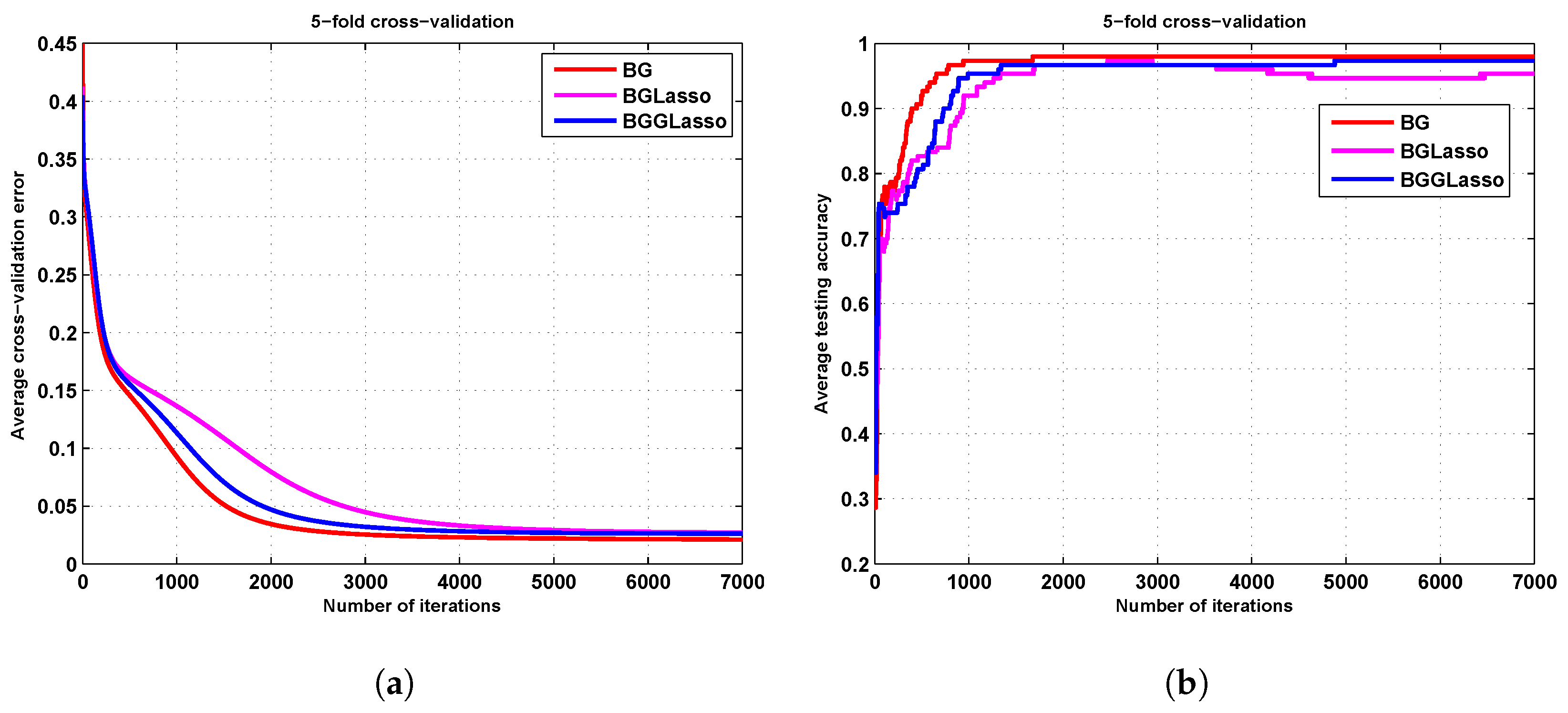
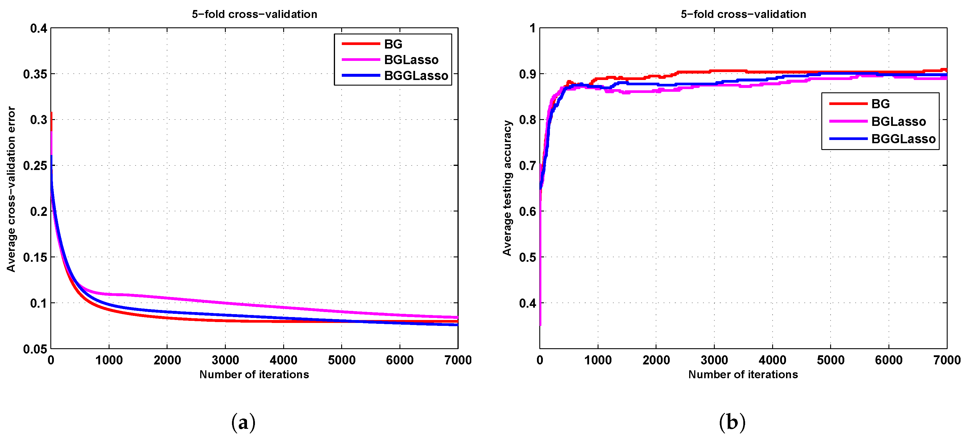
3.1. The Iris Results

The numerical results in Figure 4 represents all 5-fold results obtained by using standard BG only. We started the training process with the oversized initial network structure, namely 5 16 3 (including bias neurons in the input and hidden layers). The network was trained until the prespecified maximum number of iteration epochs of 7000 is met. We select the best learning rate η = 0.050 . In Figure 4a, we demonstrate all the training errors with their corresponding cross validation errors of all 5-folds. Similarly, in Figure 4b, all of the training accuracies with their corresponding testing accuracies of all 5-folds are demonstrated.
After this, for the sake of comparison and simplicity, we only present the best learning curves using validation sets in terms of average results. The best learning curves for average cross-validation error results and average testing accuracy of our proposed BGGLasso learning method with BG and BGLasso learning methods by using the iris dataset are displayed in Figure 5a,b, respectively. In Table 2, the average sparsity result and average accuracy result with the best learning rate η and the best regularization parameter λ over 5-fold-cross validation for the iris dataset are recorded.

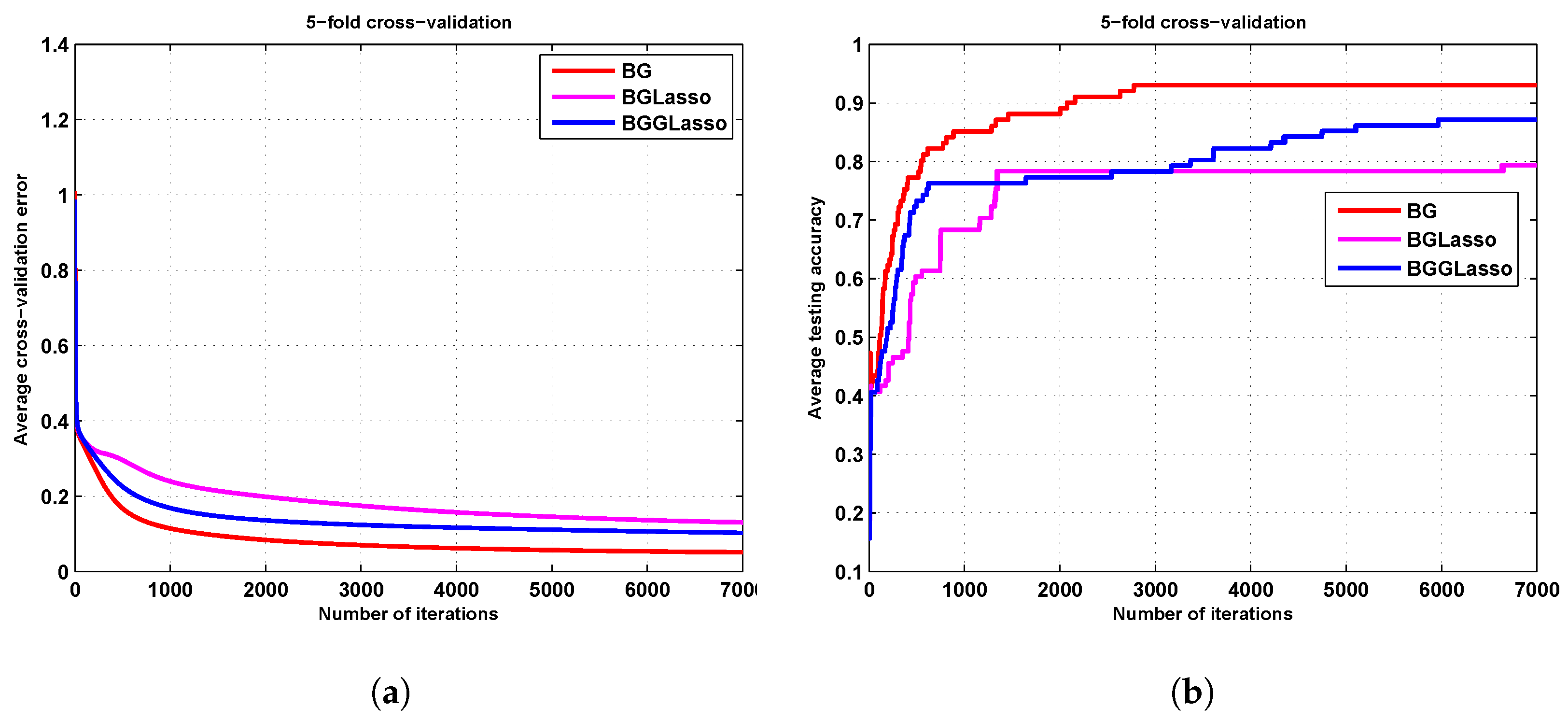
3.2. The Zoo Results

To check the sparsity ability of the group Lasso and Lasso regularization terms using the zoo dataset, we randomly started with big neural network structure 18 26 7 (the number of input neurons, the number of hidden layer neurons, and the number of output layer neurons), including the bias neurons in the input and hidden layers. For zoo dataset, the selected best learning rate η and the best regularization parameter λ are 0.040 and 0.030, respectively. The maximum number of training iteration is 7000. The best learning curves for the zoo dataset with average cross-validation error result and average testing accuracy result are shown in Figure 6a,b. Table 3 summarizes the average results with best learning parameters.

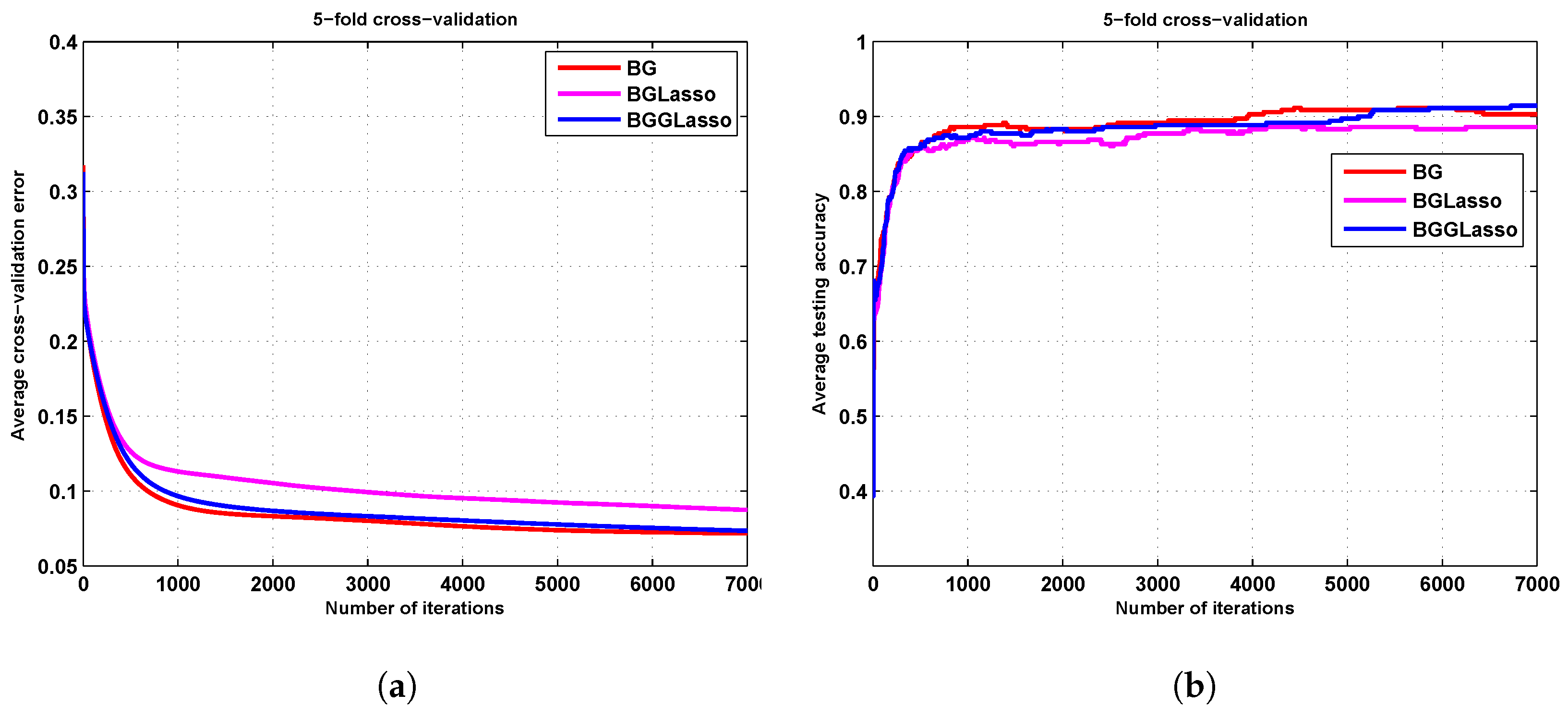
3.3. The Seed Results

Similarly, to test the sparsity ability of the group Lasso and Lasso regularization terms using the seeds dataset, we started from a large network structure 8 16 3 (including bias neurons in the input and hidden layers), and the maximum number of training epochs is 7000. The best learning rate η and the best regularization parameter λ for the seeds dataset are 0.080 and 0.009 , respectively. The best learning curves for seeds dataset with average cross-validation error results and average testing accuracy results are shown in Figure 7a,b.

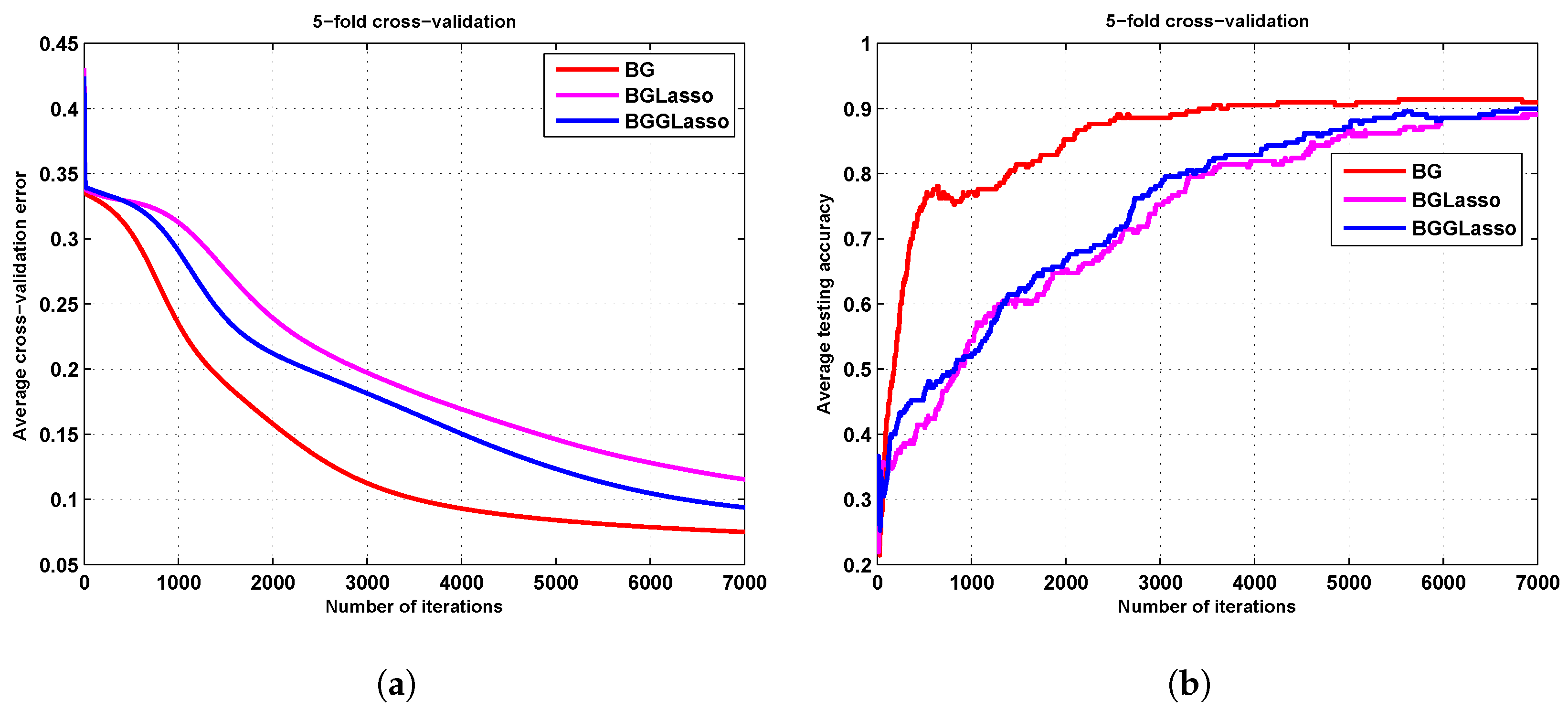
3.4. The Ionosphere Results

Here, we started with two different initial network structures ( 35 41 2 and 35 50 2 ) (each network includes bias neurons in the input and hidden layers), and both took 7000 training epochs. We trained these two different network structures with the same learning parameters and the selected best learning rate η and λ are 0.050 and 0.007, respectively. The best learning curves for cross-validation error and average testing accuracy of the first network structure are shown in Figure 8a,b, respectively. Similarly, the best learning curves for average cross-validation error and average testing accuracy of the second network structure are also shown in Figure 9a,b, respectively.

4. Discussion

The main goal of this study is to prune the redundant or unnecessary hidden layer neurons of the FNNs. In this respect, the regularization terms are often introduced into the error function and have shown to be efficient to improve the generalization performance and decrease the magnitude of the network weights [31]. In particular, L p regularizations are used to regularize the sum of the norm of the weights during training. Lasso [23] is one of the most popular L p regularization terms that is used to remove the redundant weights. However, Lasso regularization is mainly introduced for removing the redundant weights, and a neuron can be removed only if all of its outgoing weights have been close to zero. As shown in Table 2, Table 3, Table 4, Table 5 and Table 6, the batch gradient method with Lasso regularization (BGLasso) can find more redundant weights, but it cannot find any redundant hidden layer neurons.
Group Lasso [26] was used for imposing the sparsity on group level to eliminate the redundant neurons of the network. As shown in Table 2, Table 3, Table 4, Table 5 and Table 6, the batch gradient method with group Lasso regularization term (BGGLasso) can identify unnecessary or redundant hidden layer neurons. The average number of pruned hidden layer neurons (AVGNPHNs) by BGGLasso is higher for each dataset. In these tables, the average norm of the gradient of the error function E W ( W ) for our proposed learning method is also smaller than BGLasso. This tells us that the BGGLasso converges better than BGLasso. Table 4 and Table 6 are the results of ionosphere dataset using the same parameters except that the initial number of hidden layer neurons are different (i.e., 35 41 2 and 35 50 2 ), respectively. Here, we confirm that the results are not significantly different.
Moreover, Figure 5a, Figure 6a, Figure 7a, Figure 8a and Figure 9a, display comparison results of the average cross-validation error obtained by different hidden layer regularization methods for iris, zoo, seeds, and ionosphere datasets, respectively. The x-axis represents the maximum number of iterations and the y-axis represents the average cross-validation error of every iteration. As we can see from these figures, BGGLasso is monotonically decreasing and converges more quickly with a smaller cross-validation error compared to the popular BGLasso regularization method. Similarly, Figure 5b, Figure 6b, Figure 7b, Figure 8b and Figure 9b depict the average testing accuracy results of hidden layer regularization methods for iris, zoo, seeds and ionosphere datasets, respectively. In each learning curves of these figures, the x-axis represents the maximum number of iterations and y-axis represents the average testing accuracy. From these learning curves, we can see that BGGLasso always has better classification performance on the validation sets as compared to BGLasso regularization method.
As seen from the above discussion, we find that our proposed BGGLasso regularization method outperforms the existing BGLasso regularization method in all numerical results. The importance of applying BGGLasso regularization method does not only result in more sparsity in hidden layer neurons but also achieves a much better test accuracy results than BGLasso. From the results of BGGLasso in Table 2, Table 3, Table 4, Table 5 and Table 6, the number of the redundant weights and the number of the redundant hidden layer neurons are proportional. This phenomenon indicates that the batch gradient method with a group Lasso regularization term has limitations on removing weight connections from surviving hidden layer neurons. All of our numerical results are obtained by applying our proposed method using one hidden layer of FNNs. One can extend our proposed approach for sparsification of FNNs that contains any number of hidden layers.

5. Conclusions

We have developed an efficient approach to eliminate the redundant or unnecessary hidden layer neurons from a feedforward neural network. To this end, we have proposed a group Lasso regularization method by considering only the outgoing weights from each hidden layer neuron. This method can easily help us to identify that the number of redundant or unnecessary hidden layer neurons with the norm of outgoing weight connections is less than the predefined threshold value. Not only does our proposed method identify the redundant hidden neurons, but it also yields a sparse network. The numerical simulations show that our proposed method outperforms the existing learning methods on the sparsity of hidden layer neurons and the results are consistent for each benchmark dataset. One key advantage of our proposed hidden layer regularization method is that it can sparse the redundant hidden neurons. By contrast, one disadvantage of our proposed regularization method is that it cannot sparse any redundant weights from the surviving hidden layer neurons. To fill this gap, in the future, we have intended to develop more regularization methods that can ultimately solve this problem. Furthermore, we plan to test our proposed hidden layer regularization method with big datasets by using deep neural networks.

Author Contributions

H.Z.A. developed the mathematical model, carried out the numerical simulations and wrote the manuscript; W.W. advised on developing the learning algorithms and supervised the work; J.Z. contributed to analysis of the results.

Acknowledgments

This work is partially supported by the Natural Science Foundation of China: 61473059,

Conflicts of Interest

The authors declare no conflict of interest.

References

  1. Haykin, S. Neural Networks: A Comprehensive Foundation; Prentice Hall PTR: Upper Saddle River, NJ, USA, 1994. [Google Scholar]
  2. Lippmann, R. An introduction to computing with neural nets. IEEE ASSP Mag. 1987, 4, 4–22. [Google Scholar] [CrossRef]
  3. Jain, A.K.; Mao, J.; Mohiuddin, K.M. Artificial neural networks: A tutorial. Computer 1996, 29, 31–44. [Google Scholar] [CrossRef]
  4. Plawiak, P.; Tadeusiewicz, R. Approximation of phenol concentration using novel hybrid computational intelligence methods. Int. J. Appl. Math. Comput. Sci. 2014, 24, 165–181. [Google Scholar] [CrossRef] [Green Version]
  5. Hinton, G.E. Connectionist learning procedures. Artif. Intell. 1989, 40, 185–234. [Google Scholar] [CrossRef] [Green Version]
  6. Pławiak, P.; Rzecki, K. Approximation of phenol concentration using computational intelligence methods based on signals from the metal-oxide sensor array. IEEE Sens. J. 2015, 15, 1770–1783. [Google Scholar]
  7. Plagianakos, V.P.; Sotiropoulos, D.G.; Vrahatis, M.N. An Improved Backpropagation Method with Adaptive Learning Rate. In Proceedings of the 2nd International Conference on: Circuits, Systems and Computers, Iraeus, Greece, 26–28 October 1998. [Google Scholar]
  8. Rumelhart, D.E.; Hinton, G.E.; Williams, R.J. Learning representations by back-propagating errors. Nature 1986, 323, 533. [Google Scholar] [CrossRef]
  9. Wilson, D.R.; Martinez, T.R. The general inefficiency of batch training for gradient descent learning. Neural Netw. 2003, 16, 1429–1451. [Google Scholar] [CrossRef] [Green Version]
  10. Sietsma, J.; Dow, R.J. Neural net pruning-why and how. In Proceedings of the IEEE International Conference on Neural Networks, San Diego, CA, USA, 24–27 July 1988; Volume 1, pp. 325–333. [Google Scholar]
  11. Setiono, R. A penalty-function approach for pruning feedforward neural networks. Neural Comput. 1997, 9, 185–204. [Google Scholar] [CrossRef] [PubMed]
  12. Aran, O.; Yildiz, O.T.; Alpaydin, E. An Incremental Framework Based on Cross-Validation for Estimating the Architecture of a Multilayer Perceptron. IJPRAI 2009, 23, 159–190. [Google Scholar] [CrossRef]
  13. Augasta, M.G.; Kathirvalavakumar, T. A Novel Pruning Algorithm for Optimizing Feedforward Neural Network of Classification Problems. Neural Process. Lett. 2011, 34, 241–258. [Google Scholar] [CrossRef]
  14. Augasta, M.G.; Kathirvalavakumar, T. Pruning algorithms of neural networks, a comparative study. Cent. Eur. J. Comput. Sci. 2013, 3, 105–115. [Google Scholar] [CrossRef]
  15. LeCun, Y.; Denker, J.S.; Solla, S.A. Optimal brain damage. Adv. Neural Inf. Process. Syst. 1990, 2, 598–605. [Google Scholar]
  16. Hassibi, B.; Stork, D.G.; Wolff, G.J. Optimal brain surgeon and general network pruning. In Proceedings of the IEEE International Conference on Neural Networks, San Francisco, CA, USA, 28 March–1 April 1993; pp. 293–299. [Google Scholar]
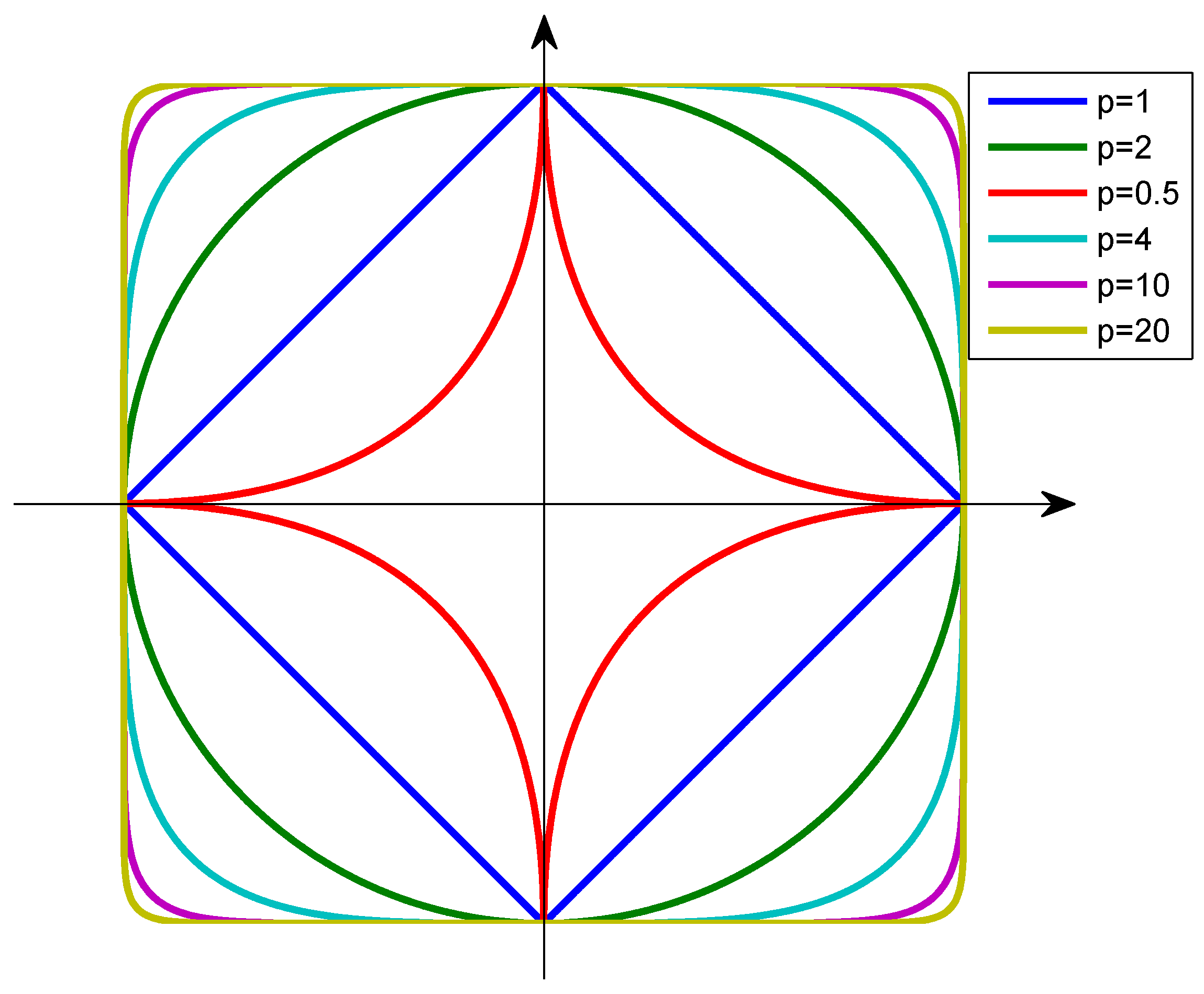
  17. Chang, X.; Xu, Z.; Zhang, H.; Wang, J.; Liang, Y. Robust regularization theory based on Lq(0 < q < 1) regularization: The asymptotic distribution and variable selection consistence of solutions. Sci. Sin. Math. 2010, 40, 985–998. [Google Scholar]
  18. Xu, Z.; Zhang, H.; Wang, Y.; Chang, X.; Liang, Y. L1/2 Regularizer. Sci. China Inf. Sci. 2010, 53, 1159–1169. [Google Scholar] [CrossRef]
  19. Wu, W.; Fan, Q.; Zurada, J.M.; Wang, J.; Yang, D.; Liu, Y. Batch gradient method with smoothing L1/2 regularization for training of feedforward neural networks. Neural Netw. 2014, 50, 72–78. [Google Scholar] [CrossRef] [PubMed]
  20. Liu, Y.; Li, Z.; Yang, D.; Mohamed, K.S.; Wang, J.; Wu, W. Convergence of batch gradient learning algorithm with smoothing L1/2 regularization for Sigma–Pi–Sigma neural networks. Neurocomputing 2015, 151, 333–341. [Google Scholar] [CrossRef]
  21. Fan, Q.; Wu, W.; Zurada, J.M. Convergence of batch gradient learning with smoothing regularization and adaptive momentum for neural networks. SpringerPlus 2016, 5, 295. [Google Scholar] [CrossRef] [PubMed]
  22. Li, F.; Zurada, J.M.; Liu, Y.; Wu, W. Input Layer Regularization of Multilayer Feedforward Neural Networks. IEEE Access 2017, 5, 10979–10985. [Google Scholar] [CrossRef]
  23. Tibshirani, R. Regression shrinkage and selection via the lasso. J. R. Stat. Soc. Ser. B (Methodol.) 1996, 58, 267–288. [Google Scholar]
  24. Yuan, M.; Lin, Y. Model selection and estimation in regression with grouped variables. J. R. Stat. Soc. Ser. B (Stat. Methodol.) 2006, 68, 49–67. [Google Scholar] [CrossRef] [Green Version]
  25. Meier, L.; Van De Geer, S.; Bühlmann, P. The group lasso for logistic regression. J. R. Stat. Soc. Ser. B (Stat. Methodol.) 2008, 70, 53–71. [Google Scholar] [CrossRef] [Green Version]
  26. Alvarez, J.M.; Salzmann, M. Learning the number of neurons in deep networks. In Advances in Neural Information Processing Systems, Proceedings of the Annual Conference on Neural Information Processing Systems, Barcelona, Spain, 5–10 December 2016; Neural Information Processing Systems Foundation, Inc.: La Jolla, CA, USA, 2016; pp. 2270–2278. [Google Scholar]
  27. Dua, D.; Taniskidou, E.K.; UCI Machine Learning Repository. University of California, Irvine, School of Information and Computer Sciences. Available online: http://archive.ics.uci.edu/ml (accessed on 14 October 2018).
  28. Rodriguez, J.D.; Perez, A.; Lozano, J.A. Sensitivity analysis of k-fold cross validation in prediction error estimation. IEEE Trans. Pattern Anal. Mach. Intell. 2010, 32, 569–575. [Google Scholar] [CrossRef] [PubMed]
  29. Han, J.; Pei, J.; Kamber, M. Data Mining: Concepts and Techniques; Elsevier: New York, NY, USA, 2011. [Google Scholar]
  30. Zhang, H.; Tang, Y.; Liu, X. Batch gradient training method with smoothing L0 regularization for feedforward neural networks. Neural Comput. Appl. 2015, 26, 383–390. [Google Scholar] [CrossRef]
  31. Reed, R. Pruning algorithms—A survey. IEEE Trans. Neural Netw. 1993, 4, 740–747. [Google Scholar] [CrossRef] [PubMed]
Figure 1. The properties of L p norms.
Symmetry 10 00525 g001
Figure 2. Feedforward neural network with one hidden layer and multiple neurons at the output layer.
Symmetry 10 00525 g002
Figure 3. K-fold cross-validation method.
Symmetry 10 00525 g003
Figure 4. Best learning curves for iris dataset only with standard BG by using η = 0.050 : (a) error and (b) accuracy.
Symmetry 10 00525 g004
Figure 5. Best learning curves for iris dataset by using BG, BGLasso and BGGLasso regularization methods with η = 0.050 , λ = 0.010 : (a) average cross-validation error and (b) average testing accuracy.
Symmetry 10 00525 g005
Figure 6. Best learning curves for zoo dataset by using BG, BGLasso and BGGLasso regularization methods with η = 0.040 , λ = 0.030 : (a) average cross-validation error and (b) average testing accuracy.
Symmetry 10 00525 g006
Figure 7. Best learning curves for seeds dataset by using BG, BGLasso and BGGLasso regularization methods with η = 0.080 , λ = 0.009 : (a) average cross-validation error and (b) average testing accuracy.
Symmetry 10 00525 g007
Figure 8. Best learning curves for ionosphere dataset by using BG, BGLasso and BGGLasso regularization methods with η = 0.050 , λ = 0.007 and network structure 35 41 2 : (a) average cross-validation error and (b) average testing accuracy.
Symmetry 10 00525 g008
Figure 9. Best learning curves for ionosphere dataset by using BG, BGLasso and BGGLasso regularization methods with η = 0.050 , λ = 0.007 and network structure 35 50 2 : (a) average cross-validation error and (b) average testing accuracy.
Symmetry 10 00525 g009
Table 1. Properties of benchmark datasets.
DatasetsNo. of ExamplesNo. of AttributesNo. of Class
Iris15043
Zoo101177
Seeds21073
Ionosphere351342
Table 2. Comparison of best average results for the iris dataset.
Methods λ η Sparsity E W ( W ) Accuracy
AVGNPWsAVGNPHNsTraining Acc. (%)Testing Acc. (%)
BG0.0000.0500.0000.0000.01098.50098.000
BGLasso0.0100.05053.2000.0000.06097.80093.300
BGGLasso0.0100.05018.4006.0000.02098.30097.300
Table 3. Comparison of best average results for zoo dataset.
Methods λ η Sparsity E W ( W ) Accuracy
AVGNPWsAVGNPHNsTraining Acc .(%)Testing Acc. (%)
BG0.0000.0400.0000.0000.020099.80093.100
BGLasso0.0300.040314.4000.0000.20086.60079.300
BGGLasso0.0300.04047.8006.8000.03093.60087.100
Table 4. Comparison of best average results for seeds dataset.
Methods λ η Sparsity E W ( W ) Accuracy
AVGNPWsAVGNPHNsTraining Acc. (%)Testing Acc. (%)
BG0.0000.0800.0000.0000.020092.50091.400
BGLasso0.0090.080101.6000.0000.06089.50089.100
BGGLasso0.0090.08024.6008.2000.04091.70090.900
Table 5. Comparison of best average results for ionosphere dataset with network structure 35 41 2 .
Methods λ η Sparsity E W ( W ) Accuracy
AVGNPWsAVGNPHNsTraining Acc. (%)Testing Acc. (%)
BG0.0000.0500.0000.0000.02098.80092.000
BGLasso0.0070.0501327.8000.0000.09094.00088.900
BGGLasso0.0070.05045.60022.8000.04097.10091.400
Table 6. Comparison of best average results for ionosphere dataset with network structure 35 50 2 .
Methods λ η Sparsity E W ( W ) Accuracy
AVGNPWsAVGNPHNsTraining Acc. (%)Testing Acc. (%)
BG0.0000.0500.0000.0000.02098.00090.900
BGLasso0.0070.0501646.4000.0000.10094.50089.800
BGGLasso0.0070.05060.40030.2000.05096.90090.000

