Transition from the Wave Equation to Either the Heat or the Transport Equations through Fractional Differential Expressions


Physics Department, Cinvestav, AP 14-740, México City 07000, Mexico
*
Author to whom correspondence should be addressed.
Symmetry 2018, 10(10), 524; https://doi.org/10.3390/sym10100524
Submission received: 29 September 2018
/
Revised: 6 October 2018
/
Accepted: 12 October 2018
/
Published: 19 October 2018
(This article belongs to the Special Issue Symmetry Breaking in Quantum Phenomena)
Abstract
:We present a model that intermediates among the wave, heat, and transport equations. The approach considers the propagation of initial disturbances in a one-dimensional medium that can vibrate. The medium is nonlinear in such a form that nonlocal differential expressions are required to describe the time evolution of solutions. Nonlocality was modeled with a space-time fractional differential equation of order in time, and order in space. We adopted the notion of Caputo for the time derivative and the Riesz pseudo-differential operator for the space derivative. The corresponding Cauchy problem was solved for zero initial velocity and initial disturbance, represented by either the Dirac delta or the Gaussian distributions. Well-known results for the conventional partial differential equations of wave propagation, diffusion, and (modified) transport processes were recovered as particular cases. In addition, regular solutions were found for the partial differential equation that arises from and . Unlike the above conventional cases, the latter equation permits the presence of nodes in its solutions.
1. Introduction
Partial differential equations play a relevant role in mathematical physics, mainly those of the second order [1,2,3,4]. In analogy to conics of analytic geometry, they are classified as either elliptic, parabolic, or hyperbolic. These equations are useful to describe a diversity of physical phenomena that include wavelike propagation, diffusion, and transport processes in practically all branches of physics. Namely, in continuous and classical mechanics, it is common to face problems of either the hyperbolic (vibrating strings, stretched membranes) or the parabolic (heat conduction) types. In statistical mechanics, to describe the motion of a cloud of noninteracting particles, it is necessary to solve a transport (linear Boltzmann) equation, which is of the parabolic type, and so on. However, as a fingerprint of the above models, the local character of the differential operators used to construct the corresponding equations permeates over the predictions. The latter produces solutions with unpleasant features from time to time because, occasionally, the predicted behavior is not compatible with the observed phenomenon. For example, the heat equation predicts that thermal disturbances propagate at infinite velocity. Clearly, the model offered by such equation is unrealistic, although it works well when diffusivity is slower than the velocity of propagation. Other examples include the study of systems that exhibit the combination of two (or more) traits. Viscoelasticity, for instance, is understood as the combination of viscous and elastic behavior exhibited by some materials when they are deformed. In such cases, the local profile of conventional differential operators represents a limitation to modeling the involved phenomena in a realistic fashion.
A form to remove the intricacies of local operators consists of substituting the usual concept of a linear medium (where the phenomenon under study is observed) by the idea of a nonlinear medium with memory. This approach has been successfully applied to change the unpleasant infinite propagation velocity of conventional diffusion by a more realistic finite velocity in, for example, [5,6]. The main point is that memory effects may be modeled with nonlocal differential equations that arise from the action of fractional differential operators on the appropriate set of functions. The same approach is useful to investigate viscoelasticity, where fractional calculus finds a great number of applications [7].
This work was undertaken to study a model that intermediates among the wave, heat, and transport equations. That is, we are interested in connecting pure wavelike propagation with pure diffusion and transport processes by means of the fractional differential properties of a single model in unified form. Our approach considers the propagation of initial disturbances in a one-dimensional medium that can vibrate. When the medium is disturbed at a given time by a vibration, perturbations spread out from the disturbance at a given velocity. The medium is considered nonlinear in such a form that nonlocality is required in both space and time variables. Thus, we studied a space-time fractional differential equation with a time derivative of order , and space derivative of order . For the time derivative, we adopted the one introduced by Caputo [8]; the space derivative is defined by the Riesz pseudo-differential operator [9]. The values taken by and define a squared area in the -plane that parameterizes the solutions of our model. Interestingly, we found regular solutions for the differential equation that arise by fixing and . Unlike the conventional equations aforementioned, this new equation permits the presence of nodes in its solutions. The zeros appear in pairs and propagate, together with the maxima and minima of the solutions, in wavelike form. As far as we know, such an equation and its solutions have been unexplored in the literature up to now. In this form, the zoology of combined phenomena may be enlarged by involving the above equation and its solutions.
The organization of the paper is as follows. Motivated by the nonlocality of fractional differential equations, in Section 2, we formulate a Cauchy problem that embraces, as particular cases, three well-known problems of mathematical physics: to solve either the (hyperbolic) wave equation, the (parabolic) heat equation, or the (modified) transport equation for properly defined initial conditions. The differential equation associated to and is a modified version of an equation of the parabolic type which completes the set of second-order partial differential equations that can be constructed by omitting the term of simultaneous space and time derivatives. Section 3 includes the solution for two different Cauchy problems, both of them considering zero initial velocity. The first one is defined by the Dirac delta distribution as the initial disturbance. The solutions are written in terms of the H-function, their convergence is analyzed, and concrete expressions are given for particular cases that include the well-known results of conventional differential equations. Some directrices about the form of intertwining such equations are also given. The second problem is defined by considering a Gaussian distribution as the initial disturbance. We show that the solution is a convergent series of H-functions. To our knowledge, this result has been missing in the literature up to now. We also show that such a series goes to the solution of the Dirac delta case at the appropriate limit. In Section 4, we include the analysis of our results and discuss the form in which the maxima of the solutions propagate in the -plane. In accordance with other studies, we found that the fractional order of the differential equations affects the behavior of the characteristic integrals in such a form that they are not straight lines anymore. However, our results show that the time dependence of the maxima is not as simple as has been reported by other authors. Some concluding remarks are included in Section 5. To offer fluidity in reading the manuscript, we have resigned detailed calculations of important solutions to Appendix B, Appendix C and Appendix D. In turn, Appendix A includes useful information and expressions that are recursively used throughout the paper.
2. Problem Formulation
The one-dimensional wave equation [1,2,3,4]
with the initial conditions
admits a unique solution given by D’Alembert’s formula
Cauchy’s problem (1) and (2) is defined for , with sufficiently smooth functions and . The first term on the right-hand side of Equation (3) represents the propagation of the initial wavelike disturbance , ruled by the characteristic integrals , for zero initial velocity . Hence, the positive parameter v represents the velocity of propagation of the wave. Consistently, propagates to the right and to the left. In turn, the integral term of Equation (3) corresponds to vibrations produced by the initial velocity with no initial disturbance .
A case of special interest is defined by the Dirac delta distribution [3] as follows:
The Initial Disturbance Equation (4) is a very localized pulse that levels off rapidly and has a strength equal to . Therefore,
is solution of the one-dimensional Wave Equation (1), with the Initial Conditions Equation (4).
On the other hand, to define uniquely the solution of the one-dimensional heat equation [1,2,3,4,10]
it is generally sufficient with the initial condition [10]
where is the absolute temperature and stands for the thermometric conductivity (or diffusivity) [10]. Any line parallel to the x-axis is a characteristic integral of Equation (6). The Cauchy problem (6) and (7) is useful to describe diffusion processes without drift in one-dimension. If the Initial Function Equation (7) is the Dirac delta distribution, then Equation (6) is the Fokker–Planck (or forward Kolmogorov) equation [11]. Indeed, it may be shown that the time-dependent Gaussian density
often called source solution [1], satisfies Equation (6) with the initial condition
Clearly, the Density Equation (8) converges to the initial distribution Equation (9) at the limit . Explicitly,
Besides, at fixed time, falls off very rapidly as increases. Therefore, the Density Equation (8) is useful to describe diffusion in one-dimensional media where the heat is concentrated in the vicinity of [4,10]. In addition, is positive and nonzero for any x and t, so one also finds that “the effect of introducing a quantity of heat at is instantaneously noticeable at remote points” [10]. That is, thermal disturbances propagate at infinite velocity. Although unrealistic, this model works well in situations where diffusivity is slower than the speed of propagation. If diffusivity and the speed of thermal waves are compatible, then Equation (6) must be modified to include an additional second-order time-derivative term [3].
One of the directions of this work is to study a model that intermediates between the wave and the heat equations described above. That is, we looked for a connection between pure wave propagation and pure diffusive phenomena in one-dimension. A first resource consists of replacing the second-order time derivative of the Wave Equation (1) by a fractional time derivative of order . In this case, we have
Here, is a constant expressed in the units , with and standing for length and time units. Using in Equation (11), we recover the Wave Equation (1) while gives the Heat Equation (6), with and respectively. Remarkably, the unpleasant feature of the Heat Equation (6)—that thermal disturbances propagate at infinite velocity—is removed since Equation (11) describes heat conduction for nonlinear materials with memory, where the speed of propagation is finite [5,6]. Extending the values of to include the sub-diffusion interval , one arrives at a fractional version of the Fokker–Planck equation for the Initial Condition Equation (9). However, such a case is out of the scope of the present work and will be studied elsewhere. Preliminary results associated to Equation (11) have been already reported by other authors in, e.g., [12,13,14,15,16,17] (see also the general approaches discussed in [7,11,18,19,20,21]).
To include a major diversity of cases, we may replace the second-order space derivative of the Heat Equation (6) by a fractional space derivative of order to obtain
The constant , measured in units , is such that . Equation (12) is useful to describe symmetric Lévy-Feller diffusion processes in which jump components are present [11,22] (see also [23,24], and general approaches in [7,11,18,19,20,21]). The parameter gives the heat equation and leads to a modified version of the one-dimensional transport equation [25,26]
It may be shown that for any smooth function , the expression solves the conventional Transport Equation; therefore, for the Initial Condition Equation (7), we have , where is the fluid (hydrodynamic) velocity [27]. The latter is not automatic for Equation (13), see [25,26]. For the sake of simplicity, Equation (13) will be referred to as Transport Equation.
The most general alternative corresponds to substituting both derivatives, the temporal and the spatial ones, by their fractional versions in Equation (1). Thus, we have the space-time fractional differential equation [25,26]
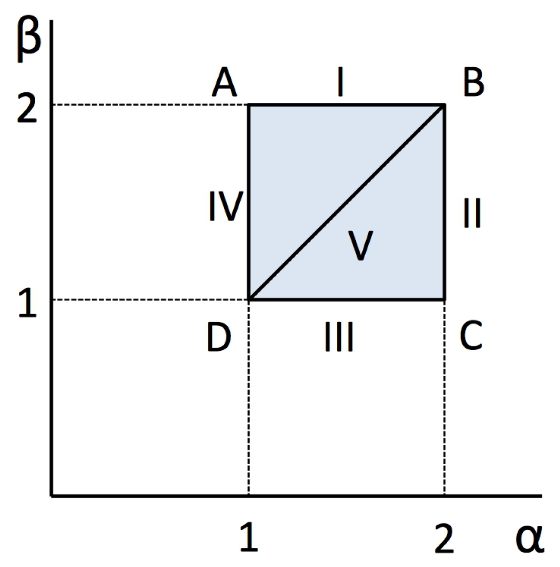
where the coupling constant is written in the units , and is such that , , and . The above equation can be studied using different approaches [7,11,18,19,20,21] and offers very interesting mathematical features, such as the fact that one can transit from the Wave Equation (1) to the Heat Equation (6), and vice versa, by fixing and running in (see segment in Figure 1). In turn, the Heat Equation (6) serves as a point of departure to arrive at the Transport Equation (13) by fixing and permitting to take values in (see segment in Figure 1). The transition from the Transport Equation (13) to the Wave Equation (1) is reached by making , with (see segment in Figure 1). Of course, any other (differentiable) path described by the point to connect B with either A or D is admissible in the -plane. As indicated above, we are interested in those paths described within the gray squared area of Figure 1, and the segment lines I-V are representative of the simplest ones. In this respect, the zone enclosed by the circuit refers to phenomena that intermediate among wave propagation, diffusive, and transport processes. The zone delimited by the circuit represents an additional resource of information. We discuss the subject in the next sections.
In addition to the differential Equations (1) and (6), together with Equation (13), we note the differential form
which is defined by the Space-Time Fractional Differential Equation (14) evaluated at vertex C, and is called the complementary equation. This can be achieved from either the Wave or the Transport Equations (1) and (13), through segment lines and , respectively. In this form, the circuit is completed as the combination of triangles and of Figure 1.
As we can see, the diversity of points that can be used to define a concrete form of Equation (14) embraces important cases of the family of second-order partial differential equations:
where the sublabels of u refer to partial derivatives in conventional notation. The term “complementary” coined for Equation (15) is then justified. In the language of linear second-order partial differential equations, the set Equation (16) includes only hyperbolic and parabolic types. Indeed, the Wave Equation (1) is hyperbolic while the Heat Equation (6) is parabolic. We shall say that Complementary and Transport Equations (15) and (13), respectively, are also “parabolic”.
3. Solution and Examples
In this section, we study the Cauchy problem defined by the Space-Time Fractional Differential Equation (14) and the Initial Conditions Equation (2). In general, we assume that the solutions will represent the propagation of initial wavelike disturbances for the initial velocity in a medium that can vibrate. That is, when the medium is disturbed at a given (initial) time by a vibration , perturbations spread out from the disturbance at initial velocity . From now on, we omit the explicit dependence of u on the parameters and for the sake of simplicity. It is expected that u will converge either to the solutions of the Wave Equation (1) or to the solutions of the Heat Equation (6) at the limits and , respectively. The same holds at the limit for the Transport Equation (13). Our main interest is in the values , with either or . In Figure 1, we show the -plane associated to the functions we are interested in.
Let us start by calculating the Laplace transform of Equation (14) in the time variable. After introducing the Initial Conditions Equation (2), we arrive at the new equation
where stands for the Laplace transform of . Now, we calculate the Fourier transform of Equation (17) in the space variable. We obtain
which is immediately solved by the function
In the above equations, we introduce the notation , , and . To retrieve U, we calculate the inverse Fourier transform
Providing the initial disturbance and velocity , the solution we are looking for is obtained from the inverse Laplace transform of (20). That is, . Next, we determine the explicit form of for and two different functions .
3.1. Delta-Like Disturbances
The straightforward calculation (see details in Appendix B) gives
where stands for the Fox function, H-function for short [28,29] (see also Appendix A). The absolute value of x in Equation (22) obeys parity properties of the Fourier transform. The full derivation of the inverse Laplace transform of Equation (22) is included in Appendix C. We obtain
Equation (23) represents the propagation of the disturbance produced by a very localized pulse in one-dimensional media, according to the Space-Time Fractional Differential Equation (14).
3.1.1. Discussion about the Convergence of Solutions
To analyze the convergence of the functions defined in Equation (23), one may consider the series expansion of the H-function given in Theorems 1.3 and 1.4 of Reference [28] (see Appendix A). It can be distinguished in two cases. For (points delimited by the triangle of Figure 1), we have the series
which converges absolutely [25]. On the other hand, for (points bordered by the triangle of Figure 1), the function acquires the form
Thus, any point in the zone defined by the circuit produces a convergent solution as in Equation (23). In turn, for the points within the triangle , the convergence of must be determined from the Series Equation (25). For instance, as produces the cancellation of the first term on the right-hand side of Equation (25), we arrive at the following expression for the points on segment line of Figure 1:
3.1.2. Special Cases
We examined the following special cases of the Function Equation (23). The sublabel of u refers to the diagram shown in Figure 1. For solutions along the segment lines I-V, we have
where is the Wright function (see Appendix A). The above expression is a well-known result for Equation (11) with the Initial Conditions Equation (4); see, e.g., [25]. We also have
According to Section 3.1.1, the above solutions are absolutely convergent series. However, although and give rise to and , respectively, they are scarcely explored in the literature. On the other hand, both of them converge to the solution associated to vertex C. That is, they lead to the solution of the Complementary Equation (15) which, in turn, seems to be missing in the set of exactly solvable differential equations that are commonly studied in physics and engineering (see, for instance, the monograph [21]).
The function
converges to and as and , respectively. As a solution of the Space-Differential Equation (12), the Expression Equation (31) is in correspondence with results that have been already reported in, e.g., [11,22,23,24]. The comparison of Equation (31) with Equation (26) gives rise to the following evaluation of the H-function:
The function
embraces the results for reported in, e.g., [25,26], and regulates the simplest transition from to and vice versa. Comparing (32) with (27), we obtain another evaluation of the H-function. Namely,
The solutions defined by the four vertices can be written as
3.1.3. Recovering Conventional Results
Wave equation. To evaluate at the limit , we use the Solution Equation (35) associated to vertex B. Of course, , , and are also useful at the appropriate limits. Using Equations (A4) and (A5) of Appendix A, we get
From (A3) of Appendix A, we see that the above integral corresponds to the inverse Mellin transform of . Then,
This last expression reproduces the solution given in Equation (5) for the one-dimensional Wave Equation (1) with the Initial Conditions Equation (4).
Heat equation. In a similar form, the limit is obtained from the Solution Equation (34) associated to vertex A. Equivalent results are obtained from either or at the appropriate limits. We have
Using the duplication formula of the Gamma Function Equation (A17), as well as the Cahen–Mellin integral Equation (A18), we arrive at the function defined in Equation (8), which is the solution of the one-dimensional Heat Equation (6) with the Initial Conditions Equation (9). The verification that satisfies the Initial Condition Equation (9) is easily achieved by using Equation (10).
- From Equation (10), we also have
Transport equation. The limit is evaluated from Equation (37), associated to vertex D (other options include either or at the appropriate limit). That is, from Equations (A4) and (A5) of Appendix A, after using the Duplication Formula Equation (A17), we have
Then, Equation (44) is reduced to the curve
which is consistent with Equation (27). The latter result is well known in the literature (see, e.g., [25], Remark 3.2). In the space variable, describes a bell-shaped curve known as either the Cauchy (mathematics), Lorentz (statistical physics), or Fock–Breit–Wigner (nuclear and particle physics) distribution [30]. It is centered at (the location parameter), with a half-width at half-maximum equal to (the scale parameter) and amplitude (height) equal to . That is, at time t, the fluid velocity defines the width of the disturbance between the half-maximum points . The function satisfies the Dirac Delta Constraints Equation (10), which can be verified at the elementary level. Therefore, Equation (45) satisfies the Transport Equation (13) with the Initial Conditions Equation (9).
Complementary equation. For and , the Series Equation (24) is simplified as follows:
Depending on the value of , the alternation of sign in , , produces pairs of zeros in that are located symmetrically with respect to . As an immediate example, for , the Series Equation (48) coincides with the peaked density
which is consistent with the initial condition . The number of zeros increases as . We will find a first pair at second order of , and so on. On the other hand, goes to zero from above as (see Equations (48) and (49)), so that the zeros produced during the propagation of the pulse are nodes of .
3.1.4. Other Representations
It is well known that the H-function embraces a large number of functions of the hypergeometric type [29]. Among the functions preferred in fractional calculus, besides the H-function, one finds Wright and Mittag–Leffler functions [7,18,19,20]. To show the flexibility of our results, in this section, we rewrite the Function Equation (23) in terms of the generalized Wright function. The translation to other hypergeometric representations is straightforward.
After changing z by , and using the duplication formula of the Gamma Function Equation (A17) in the Mellin–Barnes Integral Representation Equation (A25) of , we have
The change of variable produces
The Mellin–Barnes representation of given in Equation (50) coincides with the expression of the Green function reported in [25] for the Cauchy problem defined by Equation (14) and the initial conditions , . In agreement with our results, in [25], it was found that the concrete form of given in Equation (53) is reduced to the absolutely convergent Series Equation (24) for . Other values of and lead to the expressions discussed in Section 3.1.1 and Reference [25].
3.2. Gaussian Disturbances
The Gaussian Density Equation (8) offers a very versatile profile to define the initial condition . Namely, at arbitrary time , we can take to write
What makes the Density Equation (54) interesting as an initial condition is that, unlike the Dirac delta distribution , this is finite at for . The configuration studied in the previous sections for can be recovered from Equation (54) at the limit , as is clear from Equation (10). Additionally, we have shown that the Gaussian Density Equation (54), as well as the Dirac Delta Pulse Equation (9), can be expressed in terms of the H-function and Equations (42) and (43), respectively. The full derivation of the solution of Equation (14) with the Initial Conditions Equation (54) and is given in Appendix D. The final result can be written as the series
where
Remarkably, with the exception of the term with , the coefficients of the Series Equations (55) and (56) become zero at the limit . Therefore, we arrive at the expression
which coincides with the Solution Equation (23) of the Space-Time Fractional Differential Equation (14) with the Initial Conditions Equation (4), as expected.
4. Analysis of the Results
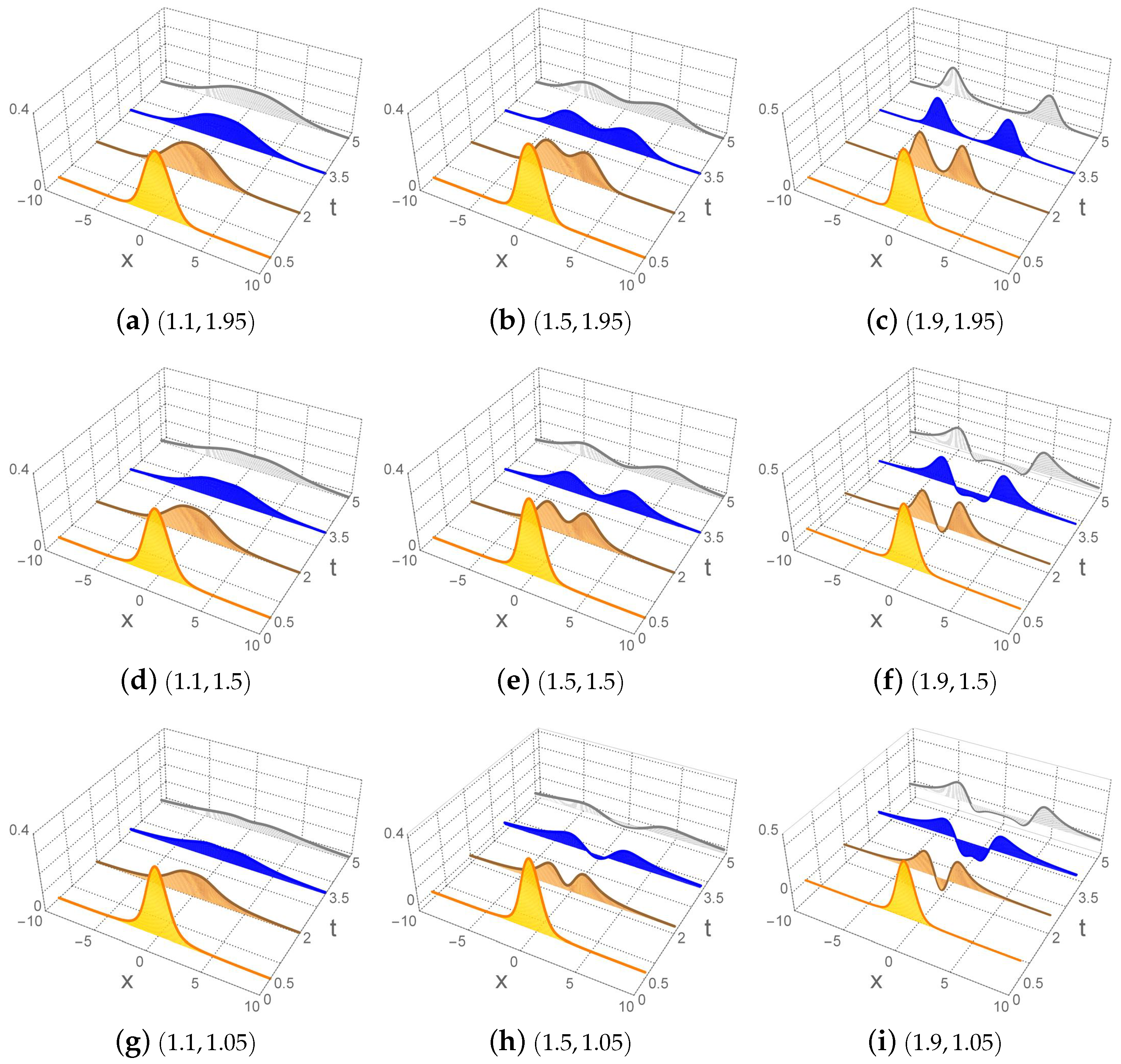
As we have indicated in the previous section, using the Gaussian Density Equation (54) as the initial condition is, in many respects, more realistic than using the Dirac Delta Distribution Equation (9). The main point is that is finite at , while diverges as . However, the disadvantage of over is that the former, although centered at , spreads along the entire x-axis, while the latter is very localized at and equal to zero for any . Nevertheless, may be recovered as a Gaussian density with an infinitesimally narrow width. In the panel of Figure 2, we show the propagation of the initial disturbance , according to the Space-Time Fractional Differential Equation (14), for different points in the gray squared area of Figure 1. The plots in Figure 2 are in correspondence with those shown in Figure 5, where we depict the propagation of the Dirac delta-like initial disturbance . That is, the behavior of the functions shown in Figure 5 may be interpreted as the form in which the functions of Figure 2 should behave at the limit .
The panel shown in Figure 2 includes the configuration for nine points of the grey square of Figure 1. We would distinguish four different situations, with Figure 2e at the barycenter. In clockwise orientation, the behavior of the group formed by Figure 2a–c,e exhibits a combination of wave propagation with diffusion. The former is stronger in (c), where is closest to vertex B, and the latter is stronger in (a), where is closest to vertex A. The clearest feature of the wave-propagation is the decoupling of the initial disturbance into two perturbations, the maxima of which evolve in time according to the respective characteristic integrals. As indicated in Section 2, these integrals are the constants for vertex B. In our case, the characteristic integrals are not straight-lines (see below for details). In turn, diffusion is characterized by the fading of the initial disturbance as time goes pass (conservation principles imply that the disturbance must spread out with time in order to preserve the area under the initial curve ). The behavior of the functions depicted in Figure 2b,e shows, with clarity, a mixture of diffusion and wave propagation.
A second group, formed by Figure 2c–i,e, shows the split of the initial disturbance into two perturbations that is characteristic of the wave-propagation. Additionally, the perturbations take negative values producing the presence of nodes as they propagate. The latter is markedly notorious in Figure 2i, where is closest to vertex C. As we have shown, such behavior is a trait of the solutions of the complementary Equation (15). Therefore, the behavior of functions included in this group is a mixture of wave- and complementary-propagation.
We have two additional groups, the behavior of which exhibits respectively a mixture of transport and complementary-propagation, and a mixture of diffusion and transport processes. The former group includes Figure 2i–g,e, and the latter is integrated by Figure 2g–a,e.
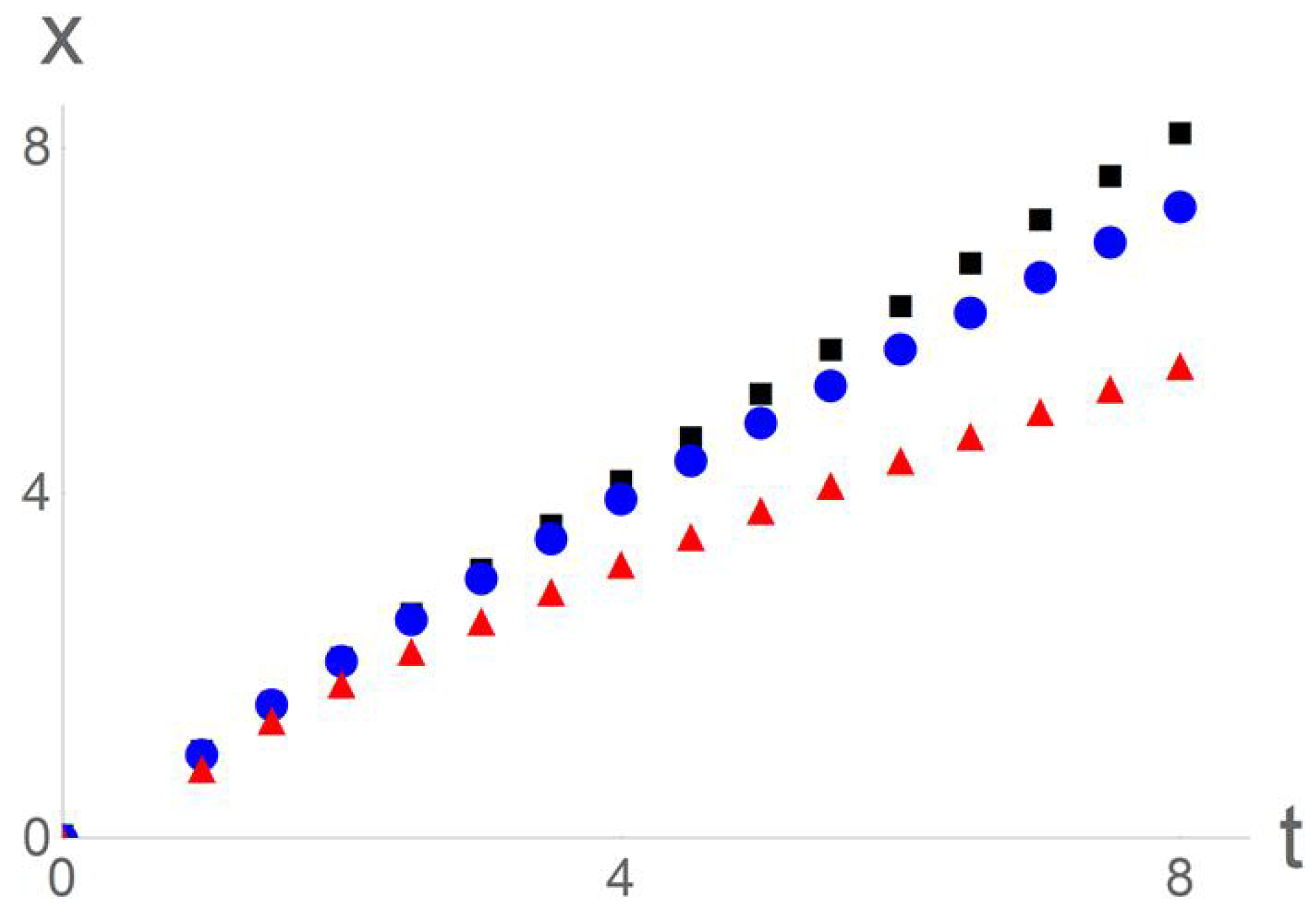
With respect to the characteristic integrals, in Figure 3 we show the distribution of the maxima of in the plane for and three different values of . That is, Figure 3 refers to the propagation of the Gaussian density defined by the points along the segment-line I. As we can see, for the characteristic integral defines a path that is almost a straight-line, which might be expected since is very close to vertex B that corresponds to the wave equation (see the pretty explanation of the behavior of characteristic integrals for wave equation in [4]). On the other hand, the path defined by is far away from a straight-line. The results depicted in Figure 3 have been calculated numerically, and obey a rule (obtained by the best-fit technique) of the form
where and are parameterized by . In contrast with other works like [14], we have found that and for . Of course, and , with .
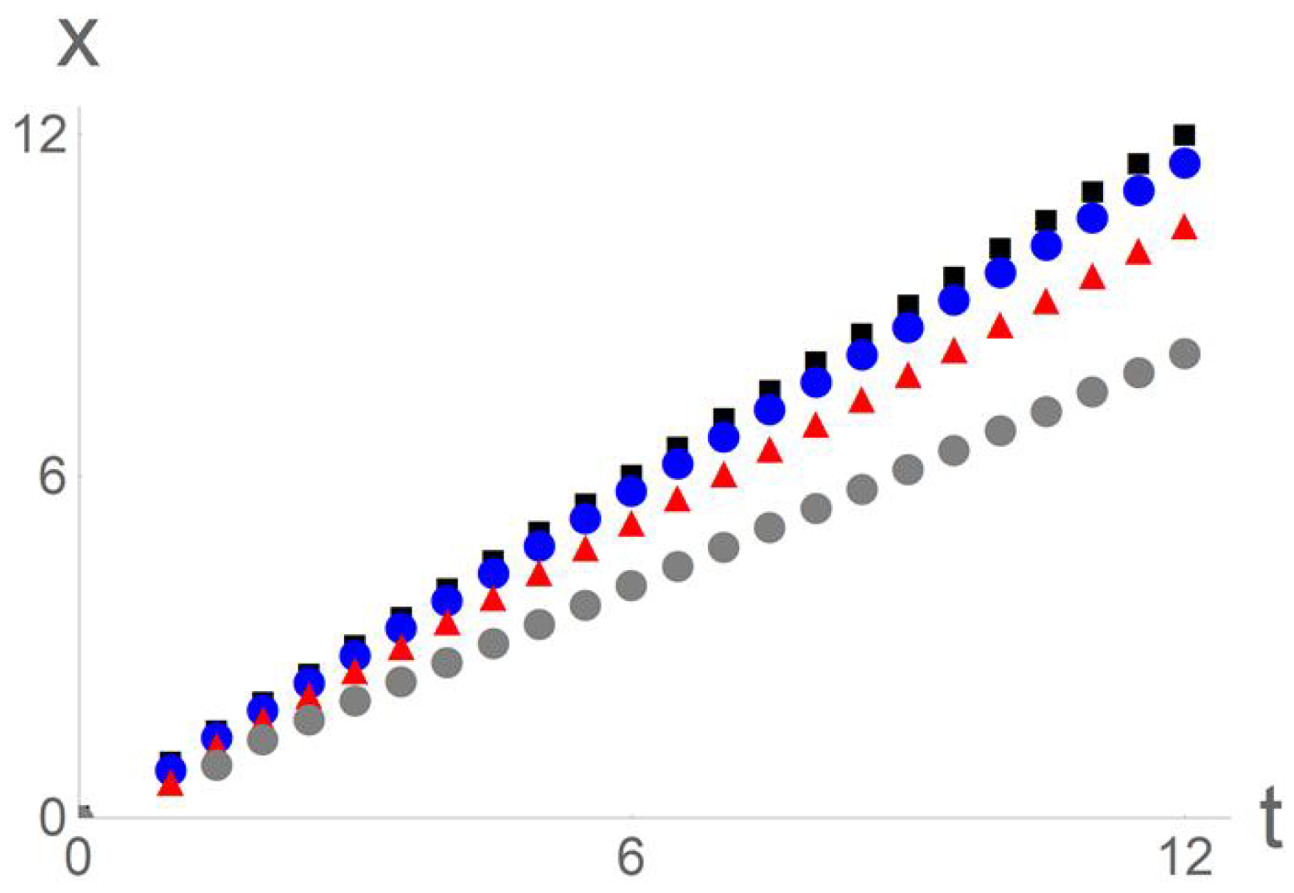
On the other hand, in Figure 4 we show the behavior of the maxima for the solutions defined along the segment-line V. In this case, we have found the rule
with and determined by . The value of is very close to that of for , as expected. As in the previous case, unlike other works [14], in our approach the rule obeyed by the maxima is not as simple as .
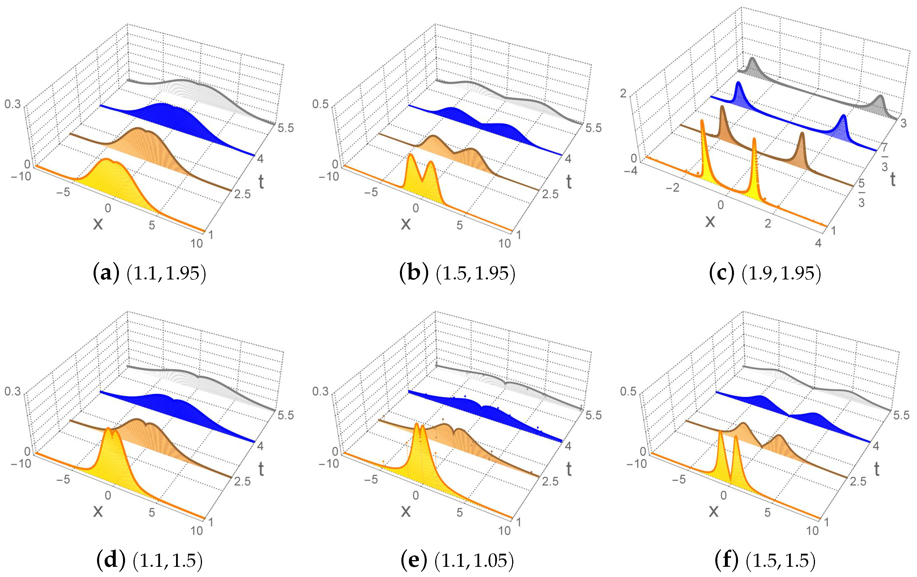
To conclude our analysis, the panel of Figure 5 shows the behavior of (23) for six different points . They correspond, in clockwise direction, to the functions depicted in Figure 2a–e,g, respectively. Here, Figure 5f s the barycenter. Unlike the Gaussian case, in the group exhibiting propagation-diffusion behavior, Figure 5a–c,f, the wavelike propagation is markedly differentiated at short times. Notice that the transport-diffusion processes are also “accelerated” in the sense that changes are presented in intervals of time that are shorter than those spent by the Gaussian profiles. A similar phenomenon is observed for the other groups (not included in Figure 5).
5. Concluding Remarks
The discussion in Section 4 motivates the addition of a new segment line in Figure 1, named , connecting the vertices A and C. Thus, defines the simplest path to transit from the Heat Equation (6) to the Complementary Equation (15). This can be written as the rule for . The presence of the new vertex E splits the square into four different triangular areas, respectively bordered by the circuits , , , and (see Figure 6). These regions of the plane are in correspondence with the groups mentioned in Section 4, so they serve to classify the solutions of the Space-Time Fractional Differential Equation (14). Namely, solutions associated to points within the region will exhibit combined properties of wavelike propagation and diffusion. Those associated to will show a mixture of wavelike and complementary propagation, and so on.
We have shown that the H-function permits to express, in unified form, a family of solutions to the Cauchy problem defined by the Space-Time Fractional Differential Equation (14) and the Initial Conditions Equation (2). We specialized to the case for two different forms of . To be concrete, we solved the problem for the Dirac Delta Pulse Equation (9) and for the Gaussian Density Equation (54) as well. We have shown that the solutions of the former can be obtained from those of the latter at the appropriate limit. In contrast with the Dirac delta distribution, which is recurrently used as the initial condition in different fractional approaches, the Gaussian density is rarely included as the initial condition in the literature on the matter. The material included in this work is addressed to fill this gap in information.
The well-known solutions of three important equations studied in mathematical physics were recovered as particular cases. We refer to the Wave Equation (1), the Heat Equation (6), and the Transport Equation (13), which respectively correspond to vertices B, A, and D of Figure 1 (see also Figure 6). In addition, we completed the set of conic-type second-order partial differential equations
by including the differential equation that results from making and in the Space-Time Fractional Differential Equation (14). That is, we solved also the differential equation associated to vertex C, the explicit form of which is introduced in Equation (15) and has been called the complementary equation throughout the present work. In this form, besides including the fractional cases where does not coincide with any vertex, our approach unifies in a single expression the solutions of four different problems that are usually treated in separate forms in mathematical physics.
Collateral results include the evaluation of different forms of the H-function. As far as we know, most of them have been unclassified up to now in the specialized literature, particularly the expressions of the H-functions in which the Dirac delta distribution is involved. We hope these results will be useful for researchers in the area.
The approach presented here may be extended to include nontrivial initial velocities . Specifically, the Dirac delta distribution offers the possibility to calculate the Green functions for the problems above mentioned. Namely, it is well known that the calculation of the Green function for a given Cauchy problem is equivalent to the calculation of the solutions to the homogeneous equation with the boundary conditions and [3]. The latter works well for vertices A, B, and D, which produce conventional partial differential equations. The verification of such a property for vertex C and any other point in the squared area is an open problem that we shall face elsewhere.
To conclude this work, we would like to emphasize that the substitution of conventional derivatives by their fractional versions in a given dynamical law produces the emergence of interactions that are not apparent (and cannot be noticed) in conventional models. The framework developed here looks for connections between different laws that are already known. However, fractional calculus offers a wider range of possibilities. For example, in the case of the harmonic oscillator, the fractional time derivative adds sorts of frictional forces that are not justified in the conventional Newtonian model since no environmental interactions are assumed a priori [31]. Therefore, the fractional version of the oscillator presupposes either that the system suffers a kind of self-interaction or that it is embedded into a medium with memory. Both assumptions predict phenomena that may require a new dynamical law for their explanation. The experiment will decide whether any of these interpretations is right. A similar situation occurs for the fractional quantum oscillator [32], for which there exist some immediate applications in quantum optics [33]. Work in this direction is in progress.
Author Contributions
Formal analysis and results, F.O.-R. and O.R.-O.; Numerical calculation and writing—original draft preparation, F.O.-R.; Conceptualization, methodology, supervision, writing—review and editing, O.R.-O.
Funding
This research was funded by Ministerio de Economía y Competitividad (Spain) grant number MTM2014-57129-C2-1-P, Consejería de Educación, Junta de Castilla y León (Spain) grant number VA057U16, and Consejo Nacional de Ciencia y Tecnología (México).
Acknowledgments
The authors are grateful to Professor L.M. Nieto for useful comments. F.O.-R. gratefully acknowledges the funding received through the CONACyT Scholarship 397335, and thanks the hospitality provided by the Department of Theoretical Physics of the University of Valladolid, Spain, where part of this work has been done.
Conflicts of Interest
The authors declare no conflict of interest. The funders had no role in the design of the study; in the collection, analyses, or interpretation of data; in the writing of the manuscript; or in the decision to publish the results.
Appendix A. Useful Definitions and Expressions
The Mellin transform [34] of a function is defined as
Consistently, the Mellin–Barnes integral (inverse Mellin transformation) is written as follows:
In particular, for , one has
The Fox function , H-function for short, is defined by the Mellin–Barnes integral
where , and q are nonnegative integers, , , and
The contour L in Equation (A4) separates the poles of , , from the poles of , . Detailed information can be found in [29].
Consider the quantity
The following theorems are reproduced from Reference [28].
Theorem A1.
(Introduced as Theorem 1.3 in [28]): Provided and , the H-function can be expanded as the series
where
and
Theorem A2.
The following expression connects the H-function with the so-called Wright function:
The H-function and the generalized Wright function are related as follows:
The duplication formula of the Gamma function is given by
The Cahen–Mellin integral [35] is defined as
Appendix B. Derivation of Equation (22)
The calculation of Equation (A19) is facilitated by the Mellin Transform Equation (A1) of . Namely,
where we have used
The integral in Equation (A22) may be determined by Equation (3.241.2) of [36] to arrive at the moment problem
which is convergent for . According to Equations (A4) and (A5) of Appendix A, the above expression corresponds to the Mellin–Barnes integral representation of an H-function. To be concrete,
which is included as Equation (22) in Section 3.1.
Appendix C. Derivation of Equation (23)
The inverse Laplace transform of is calculated at the elementary level by noticing that the s-variable, which is to be transformed, is encoded in the term appearing as a factor on the right-hand side of Equation (A24). From Equation (A20), we have
Therefore,
permits the expression of the solution in the Mellin–Barnes integral representation
From Equations (A4) and (A5) of Appendix A, we finally obtain
which corresponds to Equation (23) of Section 3.1.
Appendix D. Derivation of Equations (55) and (56)
For given in Equation (54) and , the integral Equation (20) is simplified as follows:
where we have used Equation (A20) of Appendix B. Now, assisted by Equation (A23) of Appendix B, we calculate the Mellin transform of Equation (A26) to get
After the power series expansion of the Gaussian factor in the integrand of Equation (A27), we use Equation (3.241.2) of [36] to arrive at the moment problem
which is convergent for . Calculating the inverse Laplace transform of the Mellin–Barnes integral of the above equation, with
we finally have
with
References
- Tikhonov, A.N.; Samarskii, A.A. Equations of Mathematical Physics; Pergamon Press: New York, NY, USA, 1963. [Google Scholar]
- Gustafson, K.E. Introduction to Partial Differential Equations and Hilbert Space Methods, 3rd ed.; Dover: New York, NY, USA, 1999. [Google Scholar]
- Duffy, D.G. Green’s Functions with Applications, 2nd ed.; CRC Press: Boca Raton, FL, USA, 2015. [Google Scholar]
- Borthwick, D. Introduction to Partial Differential Equations; Springer: Basel, Switzerland, 2018. [Google Scholar]
- Gurtin, M.E.; Pipkin, A.C. A general theory of heat conduction with finite wave speeds. Arch. Ration. Mech. Anal. 1968, 31, 113–126. [Google Scholar] [CrossRef]
- Miller, R.K. An integrodifferential equation for rigid heat conductors with memory. J. Math. Anal. Appl. 1978, 66, 313–332. [Google Scholar] [CrossRef]
- Mainardi, F. Fractional Calculus and Waves in Linear Viscoelasticity. An Introduction to Mathematical Models; Imperial College Press: Singapore, 2010. [Google Scholar]
- Caputo, M. Linear models of dissipation whose Q is almost frequency independent, part II. Geophys. J. R. Astr. Soc. 1967, 13, 529–539. [Google Scholar] [CrossRef]
- Riesz, M. L’integrale de Riemann-Liouville et le probléme de Cauchy. Acta Math. 1949, 81, 1–222. [Google Scholar] [CrossRef]
- Widder, D.V. The Heat Equation; Academic Press: New York, NY, USA, 1975. [Google Scholar]
- Umarov, S. Introduction to Fractional and Pseudo-Differential Equations with Singular Symbols; Springer: Basel, Switzerland, 2015. [Google Scholar]
- Wyss, W. Fractional diffusion equation. J. Math. Phys. 1986, 27, 2782–2785. [Google Scholar] [CrossRef]
- Schneider, W.R.; Wyss, W. Fractional diffusion and wave equations. J. Math. Phys. 1989, 30, 134–144. [Google Scholar] [CrossRef]
- Fujita, Y. Integrodifferential equation which interpolates the heat and the wave equations. Osaka J. Math. 1990, 27, 309–321. [Google Scholar]
- Mainardi, F. The fundamental solutions of the Fractional Diffusion Wave Equation. Appl. Math. Lett. 1996, 9, 23–28. [Google Scholar] [CrossRef]
- Mainardi, F. Fractional relaxation-oscillation and fractional diffusion-wave phenomena. Chaos Solitons Fractals 1996, 7, 1461–1477. [Google Scholar] [CrossRef]
- Mainardi, F.; Luchko, Y. Pagnini, The fundamental solution of the space-time fractional diffusion equation. Fract. Calc. Appl. Anal. 2001, 4, 153. [Google Scholar]
- Podlubny. Fractional Differential Equations; Academic Press: New York, NY, USA, 1999. [Google Scholar]
- Gorenflo, R.; Kibas, A.A.; Mainardi, F.; Rogosin, S.V. Mittag-Leffler Functions, Related Topics and Applications; Springer: Heidelberg, Germany, 2014. [Google Scholar]
- Hermann, R. Fractional Calculus—An Introduction for Physicist, 3rd ed.; World Scientific Publishing: Singapore, 2018. [Google Scholar]
- Uchaikin, V.V. Fractional Derivatives for Physics and Engineers. Volume I. Background and Theory; Springer: New York, NY, USA, 2013. [Google Scholar]
- Gorenflo, R.; Mainardi, F. Approximation to Lévy-Feller diffusion by random walk. Z. Anal. Anwend. 1999, 18, 231. [Google Scholar] [CrossRef]
- Saichev, A.; Zazlavsky, G. Fractional kinetic equations: Solutions and applications. Chaos 1997, 7, 753–764. [Google Scholar] [CrossRef] [PubMed]
- Gorenflo, E.; Mainardi, F. Random walk models for space-fractional diffusion processes. Fract. Calc. Appl. Anal. 1998, 1, 167. [Google Scholar]
- Gorenflo, R.; Iskenderov, A.; Luchko, Y. Mapping between solutions of fractional diffusion wave equations. Fract. Calc. Appl. Anal. 2000, 3, 75–86. [Google Scholar]
- Luchko, Y. Fractional wave equation and damped waves. J. Math. Phys. 2013, 54, 031505. [Google Scholar] [CrossRef]
- Medeiros-Kremer, G. An Introduction to the Boltzmann Equation and Transport Processes in Gases; Springer: Berlin, Germany, 2010. [Google Scholar]
- Kilbas, A.A. H-Transforms: Theory and Applications; CRC Press: New York, NY, USA, 2004. [Google Scholar]
- Mathai, A.M.; Saxena, R.K.; Haubold, H.J. The H-Function; Springer: New York, NY, USA, 2010. [Google Scholar]
- Rosas-Ortiz, O.; Fernández-García, N.; Cruz, Y.; Cruz, S. A primer on resonances in quantum mechanics. AIP Conf. Proc. 2008, 1077, 31–57. [Google Scholar]
- Olivar-Romero, F.; Rosas-Ortiz, O. Fractional Driven Damped Oscillator. J. Phys. Conf. Ser. 2017, 839, 012010. [Google Scholar] [CrossRef] [Green Version]
- Olivar-Romero, F.; Rosas-Ortiz, O. Factorization of the Quantum Fractional Oscillator. J. Phys. Conf. Ser. 2016, 698, 012025. [Google Scholar] [CrossRef]
- Huang, C.; Dong, L. Beam propagation management in a fractional Schrödinger equation. Sci. Rep. 2017, 7, 5442. [Google Scholar] [CrossRef] [PubMed]
- Bertrand, J.; Bertrand, P.; Ovarlez, J. The Mellin Transform. In The Transforms and Applications Handbook; Poularikas, A.D., Ed.; CRC Press: Boca Raton, FL, USA, 2000. [Google Scholar]
- Hardy, G.H.; Littlewood, J.E. Contributions to the Theory of the Riemann Zeta—Function and the Theory of the Distribution of Primes. Acta Math. 1916, 41, 119–196. [Google Scholar] [CrossRef]
- Gradshteyn, I.S.; Ryzhik, I.M. Table of Integrals, Series and Products, 7th ed.; Academic Press: New York, NY, USA, 2007. [Google Scholar]
Figure 1.
The -plane associated to the Space-Time Differential Equation (14). The square contains the points that are the subject of interest in this work. Vertices B, A, and D correspond to the Wave Equation (1), the Heat Equation (6), and the Transport Equation (13), respectively. The solutions of Equation (14) for different initial conditions (Equation (2)) associated to the gray squared area are defined within the text. Special attention is paid to the five segment lines defined by , , and , and the vertices . See complementary information in Table 1.

Figure 2.
Time evolution of the functions ue(x, t) defined in Equations (55) and (56) for points (α, β) inside the grey squared area of Figure 1. The clockwise oriented sets of figures (a)–(c), (c)–(i), (i)–(g), and (g–a) follow the segment-lines I-IV, respectively, and the set (g,e,c) follows Segment-line V. In turn, Figures (a,c,i,g) refer to points (α, β) that are very close to vertices A, B, D and C, respectively.

Figure 3.
Propagation of the (right-hand side) maxima of the solutions to the time-fractional differential Equation (11) with initial conditions Equation (54) and . We have taken defined in Equations (55) and (56) with , see Figure 2. The plots correspond to (solid square, black), (disk, blue) and (solid triangle, red).

Figure 4.
Propagation of the (right-hand side) maxima of the functions defined in Equations (55) and (56) for , see Figure 2. The plots correspond to (solid square, black), (disk, blue), (solid triangle, red), and (disk, grey).

Figure 5.
Time evolution of the functions u(x, t) defined in Equation (23) for the indicated values of the pair (α, β) inside the circuit BAD of Figure 1. The panel is clockwise oriented. Solutions in the upper row are very close to uI(x, t), defined in Equation (28), and follow a path parallel to the segment line I. Figure (c,f,e) follow a path parallel to the segment line V. The circuit is closed with Figure (e,d,a), which follow a path parallel to the segment line IV.

Figure 6.
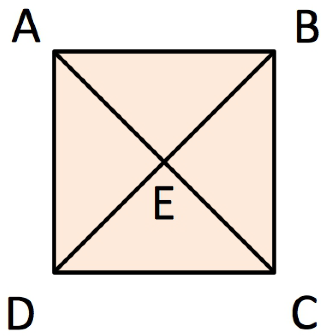
The square of Figure 1 with an additional segment line that connects the vertices A and C. The addition of vertex E splits the square into four different triangular areas that serve to classify the solutions of the Space-Time Fractional Differential Equation (14) according to their properties. Clockwise oriented, with vertex E as the barycenter, points within the area delimited by the circuit define solutions with combined properties i and j, where i and j stand for A (heat diffusion), B (wave propagation), C (complementary propagation), and D (transport process). See Discussion in Section 4.
Figure 6.
The square of Figure 1 with an additional segment line that connects the vertices A and C. The addition of vertex E splits the square into four different triangular areas that serve to classify the solutions of the Space-Time Fractional Differential Equation (14) according to their properties. Clockwise oriented, with vertex E as the barycenter, points within the area delimited by the circuit define solutions with combined properties i and j, where i and j stand for A (heat diffusion), B (wave propagation), C (complementary propagation), and D (transport process). See Discussion in Section 4.


Table 1.
The four differential equations defined by Equation (14) for the vertices can be intertwined by paths described in the squared area . The simplest transition from one of them to any other is achieved through the Solutions Equation (23) associated to the five segment lines I-V shown in Figure 1.
| Fractional Expression | Simplest Transition | Involved Equations |
|---|---|---|
| wave ↔ heat | ||
| Equation (28) | Equation (35) ↔ Equation (34) | Equation (1) ↔ Equation (6) |
| heat ↔ transport | ||
| Equation (31) | Equation (34) ↔ Equation (37) | Equation (6) ↔ Equation (13) |
| transport ↔ wave | ||
| Equation (32) | Equation (37) ↔ Equation (35) | Equation (13) ↔ Equation (1) |
| wave ↔ compl. | ||
| Equation (29) | Equation (35) ↔ Equation (36) | Equation (1) ↔ Equation (15) |
| compl. ↔ transport | ||
| Equation (30) | Equation (36) ↔ Equation (37) | Equation (15) ↔ Equation (13) |
© 2018 by the authors. Licensee MDPI, Basel, Switzerland. This article is an open access article distributed under the terms and conditions of the Creative Commons Attribution (CC BY) license (http://creativecommons.org/licenses/by/4.0/).
Share and Cite
MDPI and ACS Style
Olivar-Romero, F.; Rosas-Ortiz, O. Transition from the Wave Equation to Either the Heat or the Transport Equations through Fractional Differential Expressions. Symmetry 2018, 10, 524. https://doi.org/10.3390/sym10100524
AMA Style
Olivar-Romero F, Rosas-Ortiz O. Transition from the Wave Equation to Either the Heat or the Transport Equations through Fractional Differential Expressions. Symmetry. 2018; 10(10):524. https://doi.org/10.3390/sym10100524
Chicago/Turabian StyleOlivar-Romero, Fernando, and Oscar Rosas-Ortiz. 2018. "Transition from the Wave Equation to Either the Heat or the Transport Equations through Fractional Differential Expressions" Symmetry 10, no. 10: 524. https://doi.org/10.3390/sym10100524
Note that from the first issue of 2016, this journal uses article numbers instead of page numbers. See further details here.