Synthetic Medical Images Using F&BGAN for Improved Lung Nodules Classification by Multi-Scale VGG16


Abstract
:1. Introduction
2. Related Work
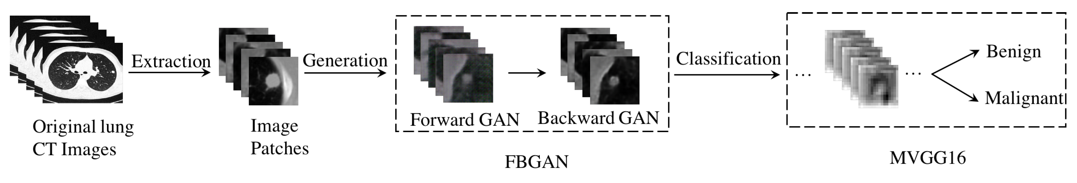
3. Methodology
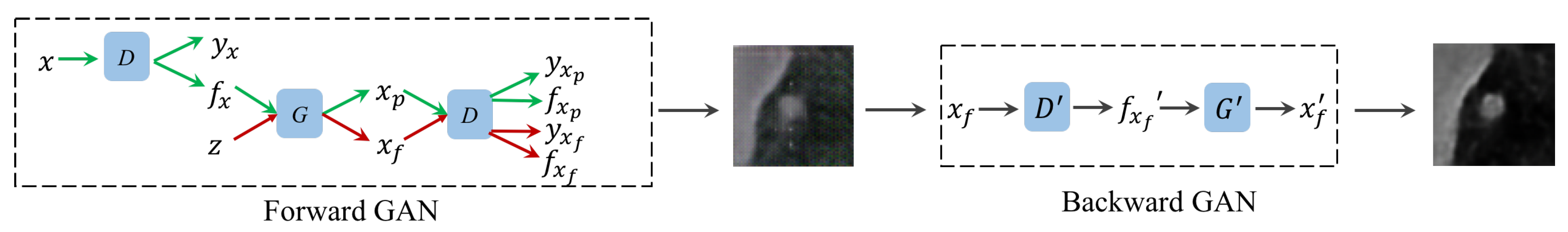
3.1. F&BGAN for Data Augmentation
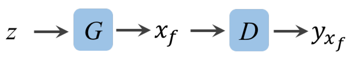
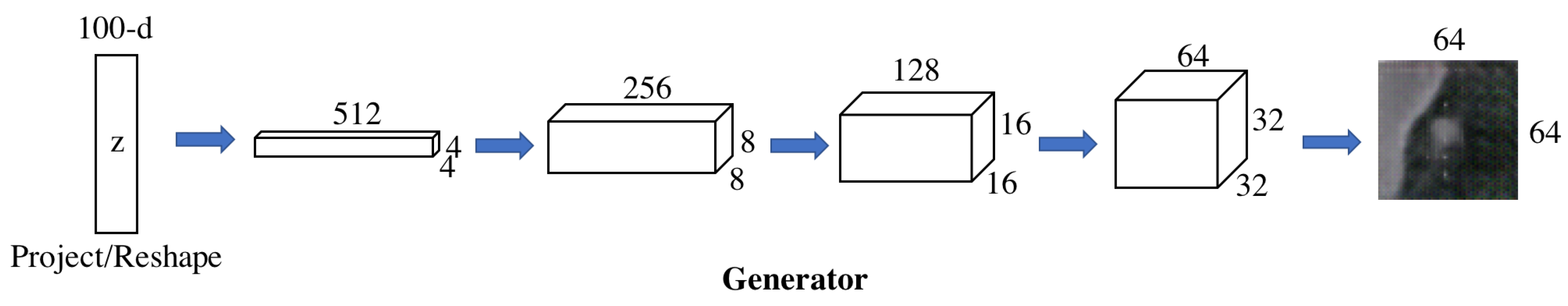
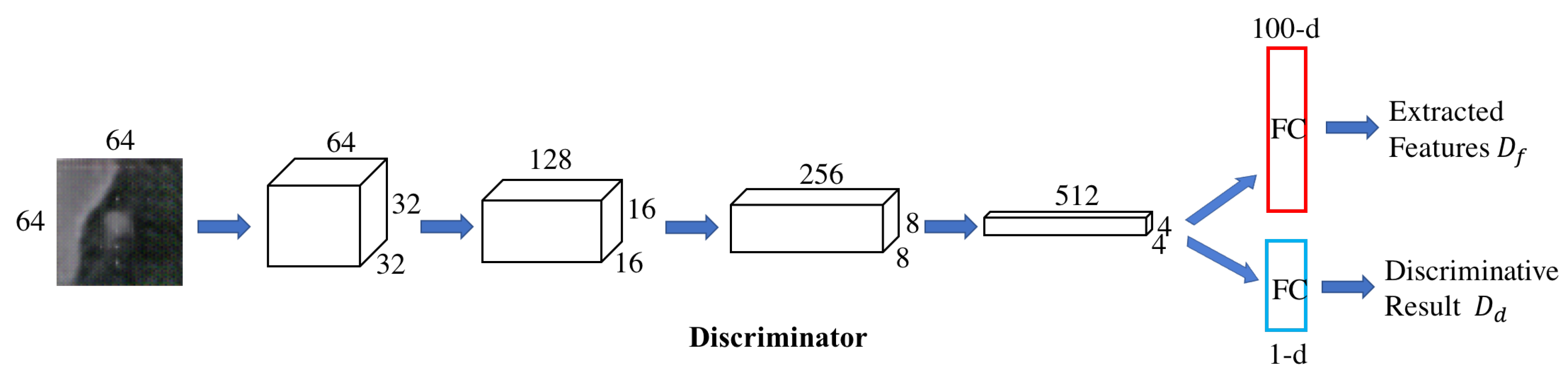
3.1.1. Forward GAN.
| Algorithm 1 The training pipeline of the proposed Forward GAN algorithm. |
| Require:m, the batch size. , initial D network parameters. , initial G network parameters. for number of training iteration do Sample x ∼ a batch from the real data; , ← Sample z ∼ a batch of random noise; ← ← , , . Calculate reconstruction loss between x and : Update discriminator D by stochastic gradient descent: − Update generator G by stochastic gradient descent: end for |
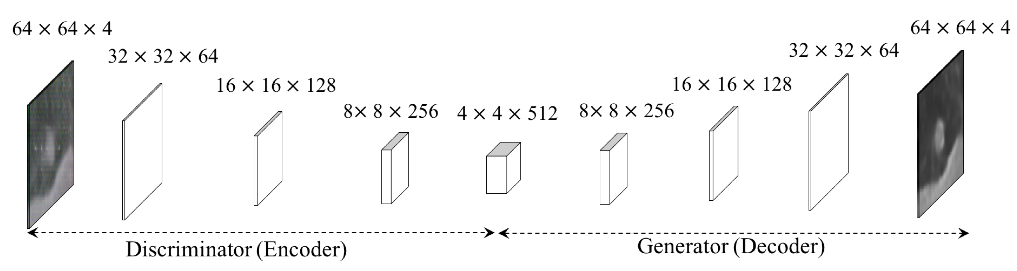
3.1.2. Backward GAN.
| Algorithm 2 The training pipeline of the proposed Backward GAN algorithm. |
| Require:m, the batch size. , initial network parameters. , initial network parameters. for number of training iteration do Sample a batch from the noise data; Sample a batch from the clear data; Update discriminator and generator by stochastic gradient descent: end for |
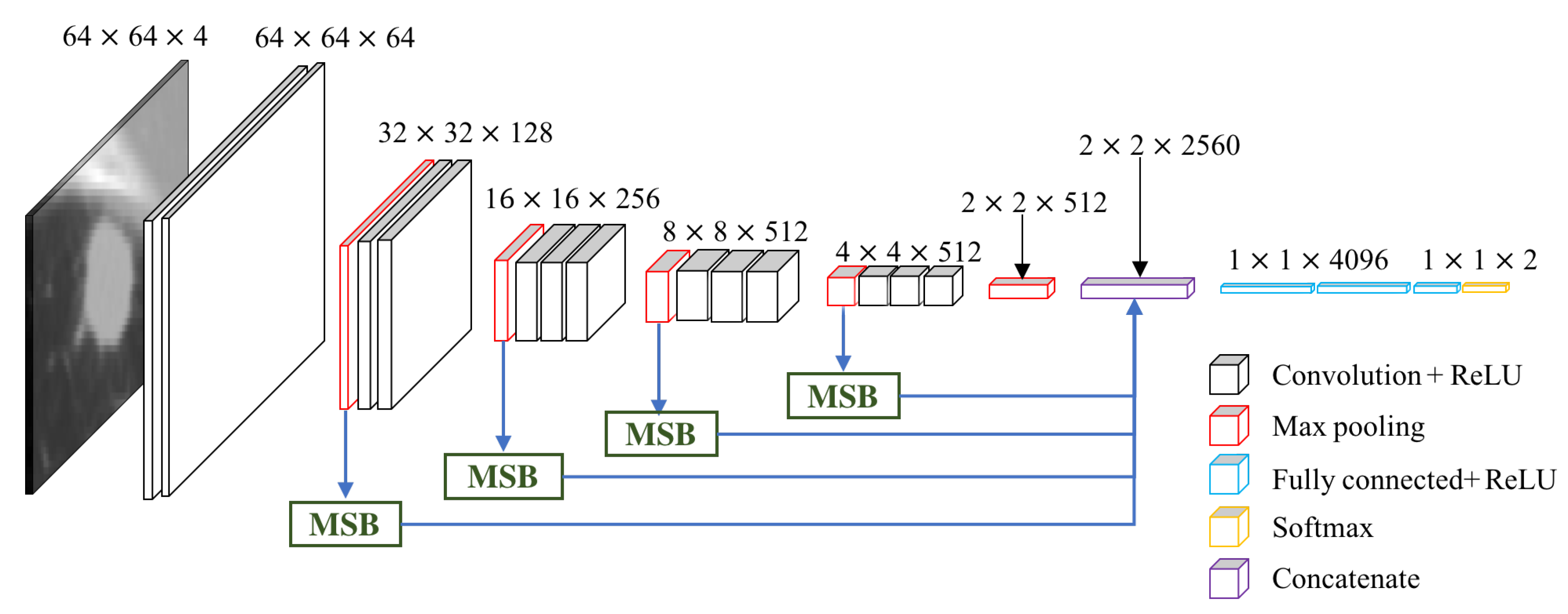
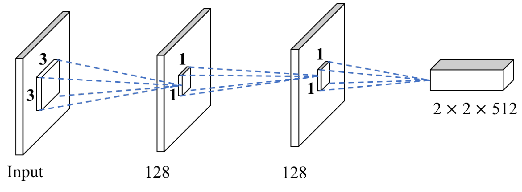
3.2. Multi-scale VGG16
4. Experiments and Results
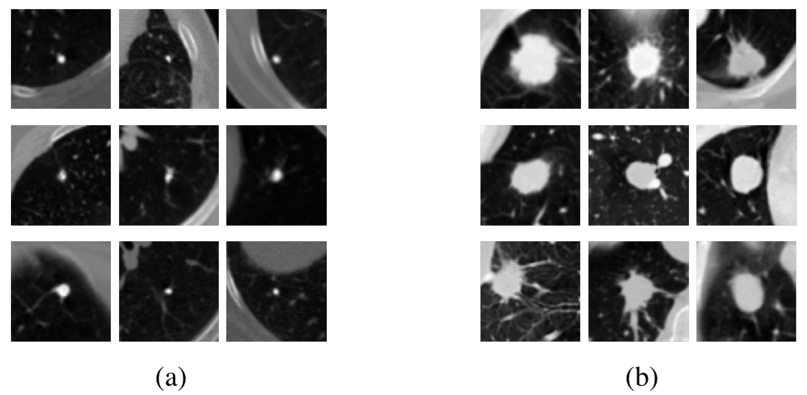
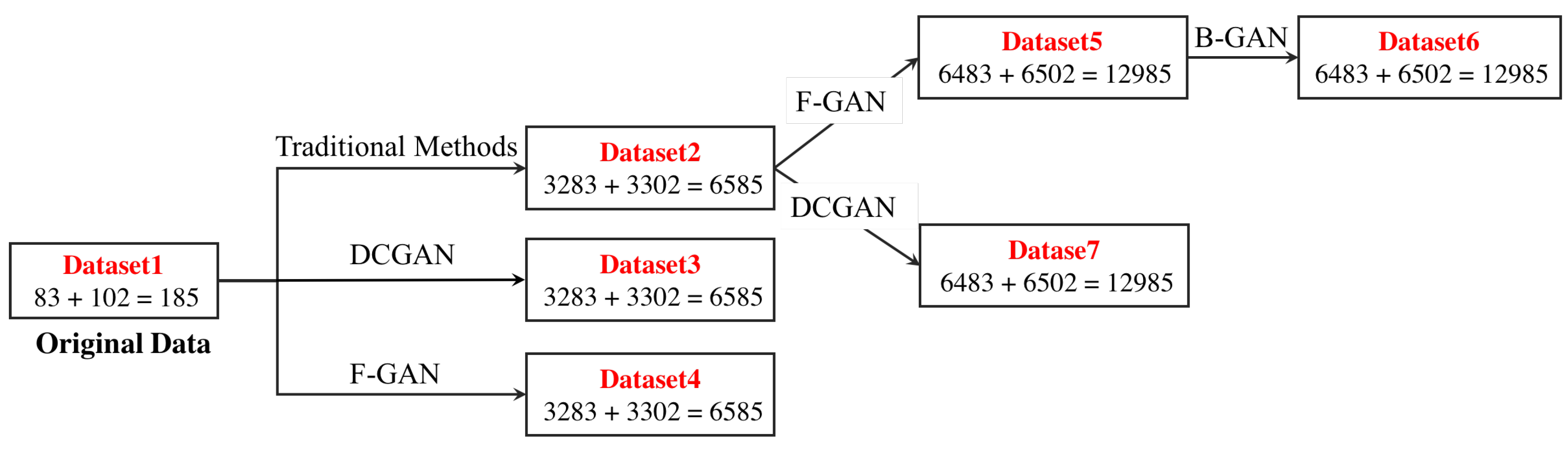
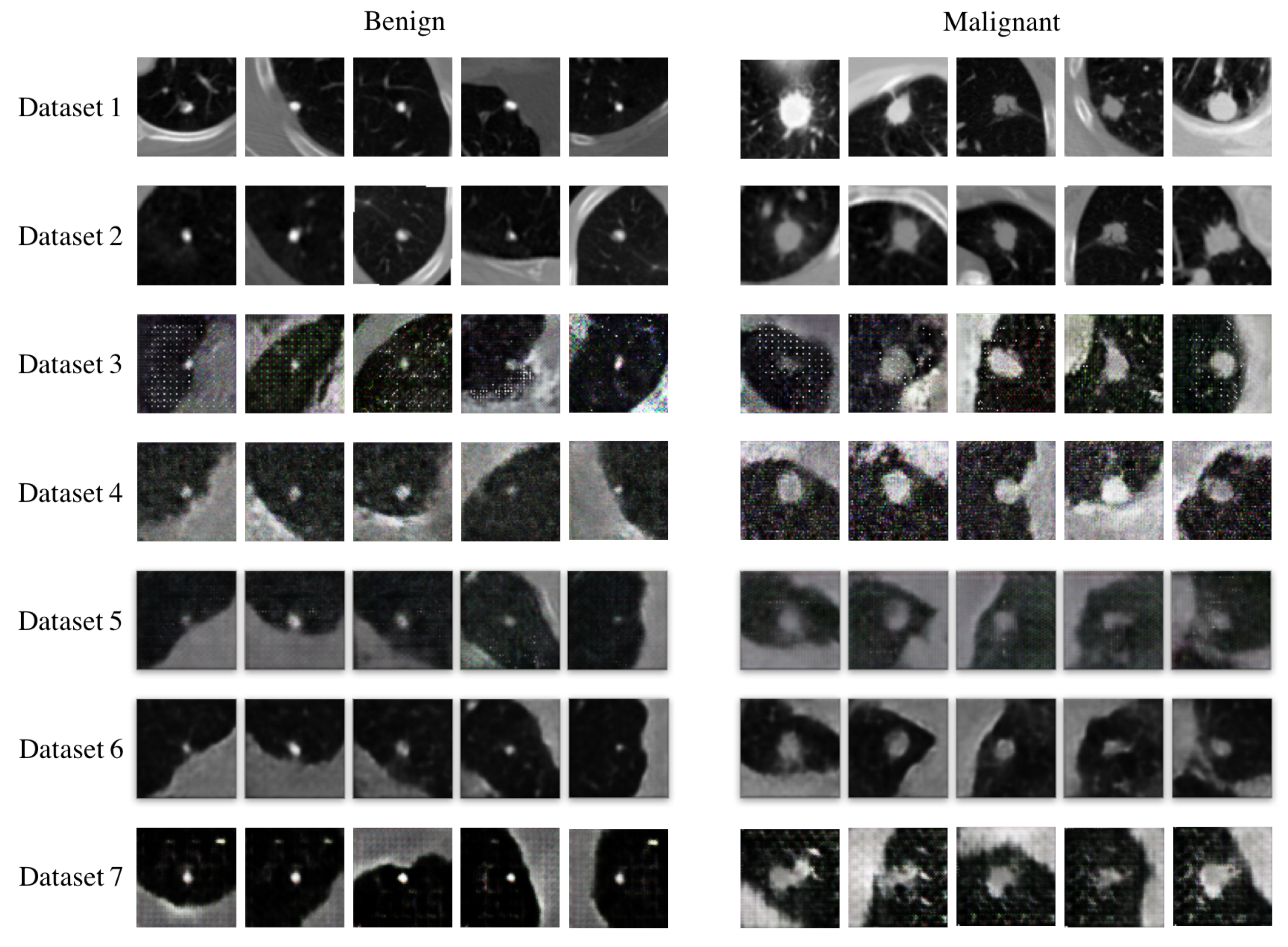
4.1. Datasets
4.2. Evaluation Metrics
- Accuracy: The accuracy is the ability of our model to differentiate the malignant and benign samples correctly. Mathematically, this can be defined as:
- Sensitivity: The sensitivity represents the ability of our model to determine the malignant samples correctly. Mathematically, this can be defined as:
- Specificity: The specificity illustrates the ability of our model to determine the benign samples correctly. Mathematically, this can be defined as:
- AUROC: the ROC curve is a graphical plot that illustrates the diagnostic ability of a binary classifier system. The AUROC score is the area under the ROC curve.
4.3. Data Augmentation Performance of F&BGAN
4.4. Classification Performance of M-VGG16
4.5. Performance of MSB
4.6. Comparison with Other Classification Methods
4.7. Comparison with the State-Of-the-Art
5. Conclusions
Author Contributions
Funding
Acknowledgments
Conflicts of Interest
References
- Jemal, A.; Siegel, R.; Ward, E.; Murray, T.; Samuels, A.; Tiwari, R.C.; Ghafoor, A.; Feuer, E.J.; Thun, M.J. Cancer statistics. CA Cancer J. Clin. 2008, 58, 71–96. [Google Scholar] [CrossRef] [PubMed]
- Ramaswamy, S.; Truong, K. Pulmonary Nodule Classification with Convolutional Neural Networks. Comput. Math. Methods Med. 2016. [Google Scholar] [CrossRef]
- Farag, A.; Ali, A.; Graham, J.; Farag, A.; Elshazly, S.; Falk, R. Evaluation of geometric feature descriptors for detection and classification of lung nodules in low dose CT scans of the chest. In Proceedings of the 2011 IEEE International Symposium on Biomedical Imaging: From Nano to Macro, Chicago, IL, USA, 30 March–2 April 2011; pp. 169–172. [Google Scholar]
- Orozco, H.M.; Villegas, O.O.V.; Domínguez, H.J.O.; Domínguez, H.D.J.O.; Sanchez, V.G.C. Lung nodule classification in CT thorax images using support vector machines. In Proceedings of the 2013 12th Mexican International Conference on Artificial Intelligence (MICAI), Mexico City, Mexico, 24–30 November 2013; pp. 277–283. [Google Scholar]
- Parveen, S.S.; Kavitha, C. Classification of lung cancer nodules using SVM Kernels. Int. J. Comput. Appl. 2014, 95, 975–8887. [Google Scholar]
- Krewer, H.; Geiger, B.; Hall, L.O.; Goldgof, D.B.; Gu, Y.; Tockman, M.; Gillies, R.J. Effect of texture features in computer aided diagnosis of pulmonary nodules in low-dose computed tomography. In Proceedings of the 2013 IEEE International Conference on Systems, Man, and Cybernetics (SMC), Manchester, UK, 13–16 October 2013; pp. 3887–3891. [Google Scholar]
- Shen, W.; Zhou, M.; Yang, F.; Yu, D.; Dong, D.; Yang, C.; Zang, Y.; Tian, J. Multi-crop convolutional neural networks for lung nodule malignancy suspiciousness classification. Pattern Recogn. 2017, 61, 663–673. [Google Scholar] [CrossRef]
- Hua, K.L.; Hsu, C.H.; Hidayati, S.C.; Hidayati, S.C.; Cheng, W.H.; Chen, Y.J. Computer-aided classification of lung nodules on computed tomography images via deep learning technique. OncoTargets Ther. 2015, 8, 2015–2022. [Google Scholar]
- Dandıl, E.; Çakiroğlu, M.; Ekşi, Z.; Özkan, M.; Kurt, Ö.K.; Canan, A. Artificial neural network-based classification system for lung nodules on computed tomography scans. In Proceedings of the 2014 6th International Conference of Soft Computing and Pattern Recognition (SoCPar), Tunis, Tunisia, 11–14 August 2014; pp. 382–386. [Google Scholar]
- Kumar, D.; Wong, A.; Clausi, D.A. Lung nodule classification using deep features in CT images. In Proceedings of the 2015 12th Conference on Computer and Robot Vision (CRV), Halifax, NS, Canada, 3–5 June 2015; pp. 133–138. [Google Scholar]
- Cheng, J.Z.; Ni, D.; Chou, Y.H.; Qin, J.; Tiu, C.M.; Chang, Y.C.; Huang, C.S.; Shen, D.; Chen, C.M. Computer-aided diagnosis with deep learning architecture: Applications to breast lesions in US images and pulmonary nodules in CT scans. Sci. Rep. 2016, 6, 24454. [Google Scholar] [CrossRef] [PubMed]
- Shen, W.; Zhou, M.; Yang, F.; Yang, C.; Tian, J. Multi-scale convolutional neural networks for lung nodule classification. In Proceedings of the International Conference on Information Processing in Medical Imaging, Cham, Switzerland, 28 June–3 July 2015; pp. 588–599. [Google Scholar]
- Kwajiri, T.L.; Tezukam, T. Classification of Lung Nodules Using Deep Learning. Trans. Jpn. Soc. Med. Biol. Eng. 2017, 55, 516–517. [Google Scholar]
- Abbas, Q. Lung-Deep: A Computerized Tool for Detection of Lung Nodule Patterns using Deep Learning Algorithms. Lung 2017, 8. [Google Scholar] [CrossRef]
- Da Silva, G.L.F.; da Silva Neto, O.P.; Silva, A.C.; Gattass, M. Lung nodules diagnosis based on evolutionary convolutional neural network. Multimed. Tools Appl. 2017, 76, 19039–19055. [Google Scholar] [CrossRef]
- Goodfellow, I.; Pouget-Abadie, J.; Mirza, M.; Xu, B.; Warde-Farley, D.; Ozair, S.; Courville, A.; Bengio, Y. Generative adversarial nets. Mach. Learn. 2014, arXiv:1406.2661, 2672–2680. [Google Scholar]
- Frid-Adar, M.; Klang, E.; Amitai, M.; Goldberger, C.; Greenspan, H. Synthetic data augmentation using GAN for improved liver lesion classification. In Proceedings of the 2018 IEEE 15th International Symposium on Biomedical Imaging (ISBI 2018), Washington, DC, USA, 4–7 April 2018; pp. 289–293. [Google Scholar]
- Guibas, J.T.; Virdi, T.S.; Li, P.S. Synthetic Medical Images from Dual Generative Adversarial Networks. arXiv, 2017; arXiv:1709.01872. [Google Scholar]
- Chuquicusma, M.J.M.; Hussein, S.; Burt, J.; Bagci, U. How to fool radiologists with generative adversarial networks? A visual turing test for lung cancer diagnosis. In Proceedings of the 2018 IEEE 15th International Symposium on Biomedical Imaging (ISBI 2018), Washington, DC, USA, 4–7 April 2018; pp. 240–244. [Google Scholar]
- Radford, A.; Metz, L.; Chintala, S. Unsupervised representation learning with deep convolutional generative adversarial networks. arXiv, 2016; arXiv:1511.06434. [Google Scholar]
- Dumoulin, V.; Belghazi, I.; Poole, B.; Mastropietro, O.; Lamb, A.; Arjovsky, M.; Courville, A. Adversarially learned inference. arXiv, 2016; arXiv:1606.00704. [Google Scholar]
- Donahue, J.; Krähenbühl, P.; Darrell, T. Adversarial feature learning. arXiv, 2016; arXiv:1605.09782. [Google Scholar]
- Simonyan, K.; Zisserman, A. Very deep convolutional networks for large-scale image recognition. arXiv, 2014; arXiv:1409.1556. [Google Scholar]
- Lowe, D.G. Object recognition from local scale-invariant features. In Proceedings of the Seventh IEEE International Conference on Computer Vision, Corfu, Greece, 20–27 September 1999; pp. 1150–1157. [Google Scholar]
- Armato, S.G., III; McLennan, G.; Bidaut, L.; McNitt-Gray, M.F.; Meyer, C.R.; Reeves, A.P.; Zhao, B.; Aberle, D.R.; Henschke, C.I.; Hoffman, E.A.; et al. The lung image database consortium (LIDC) and image database resource initiative (IDRI): A completed reference database of lung nodules on CT scans. Med. Phys. 2011, 38, 915–931. [Google Scholar] [PubMed]
- Farag, A.; Elhabian, S.; Graham, J.; Farag, A.; Falk, R. Toward precise pulmonary nodule descriptors for nodule type classification. In Proceedings of the International Conference on Medical Image Computing and Computer-Assisted Intervention, Granada, Spain, 16–20 September 2010; pp. 626–633. [Google Scholar]
- Ojala, T.; Pietikäinen, M.; Harwood, D. A comparative study of texture measures with classification based on featured distributions. Pattern Recognit. 1996, 29, 51–59. [Google Scholar] [CrossRef]
- Cortes, C.; Vapnik, V. Support-vector networks. Mach. Learn. 1995, 20, 273–297. [Google Scholar] [CrossRef] [Green Version]
- Altman, N.S. An introduction to kernel and nearest-neighbor nonparametric regression. Am. Stat. 1992, 46, 175–185. [Google Scholar]
- Krizhevsky, A.; Sutskever, I.; Hinton, G.E. Imagenet classification with deep convolutional neural networks. In Proceedings of the Advances in neural information processing systems, Lake Tahoe, NV, USA, 3–6 December 2012; pp. 1097–1105. [Google Scholar]
- Szegedy, C.; Liu, W.; Jia, Y.; Sermanet, P.; Reed, S.; Anguelov, D.; Erhan, D.; Vanhoucke, V.; Rabinovich, A. Going deeper with convolutions. In Proceedings of the IEEE Conference on Computer Vision and Pattern Recognition, Boston, MA, USA, 7–12 June 2015; pp. 1–9. [Google Scholar]
- He, K.; Zhang, X.; Ren, S.; Sun, J. Deep residual learning for image recognition. In Proceedings of the IEEE Conference on Computer Vision and Pattern Recognition, Las Vegas, NV, USA, 27–30 June 2016; pp. 770–778. [Google Scholar]
- Nanni, L.; Ghidoni, S.; Brahnam, S. Handcrafted vs. non-handcrafted features for computer vision classification. Pattern Recognit. 2017, 71, 158–172. [Google Scholar] [CrossRef]


| Approach | Author | Year | Method |
|---|---|---|---|
| Traditional | Farag et al. [3] | 2011 | Texture features and KNN. |
| Orozco et al. [4] | 2013 | Eight texture features and SVM. | |
| Krewer et al. [6] | 2013 | Texture and shape features with DT, KNN, and SVM. | |
| Parveen and Kavitha [5] | 2014 | Use GLCM to extract features and SVM to classify. | |
| Neural network | Dandil et al. [9] | 2014 | ANNs for classification. |
| Hua et al. [8] | 2015 | DBN and CNN for classification. | |
| Kumar et al. [10] | 2015 | SAE for classification. | |
| Shen et al. [12] | 2015 | Multi-scale CNN (MCNN) for classification. | |
| Cheng et al. [11] | 2016 | SDAE for classification. | |
| Shen et al. [7] | 2017 | Multi-crop CNN (MC-CNN) for classification. | |
| Kwajiri and Tezuka [13] | 2017 | CNN and ResNet to classify. | |
| Abbas [14] | 2017 | Integrate CNN and RNN for classification. | |
| da Silva et al. [15] | 2017 | Evolutionary CNN for classification. |
| Layer | Input | Output | Filter Size | Strides | |
|---|---|---|---|---|---|
| MSB1 | conv1 | 32 × 32 × 64 | 8× 8 × 128 | 3 | 4 |
| conv2 | 8 × 8 × 128 | 4 × 4 × 128 | 1 | 2 | |
| conv3 | 4 × 4 × 128 | 2 × 2 × 512 | 1 | 2 | |
| MSB2 | conv1 | 16 × 16 × 128 | 4 × 4 × 128 | 3 | 4 |
| conv2 | 4 × 4 × 128 | 2 × 2 × 128 | 1 | 2 | |
| conv3 | 2 × 2 × 128 | 2 × 2 × 512 | 1 | 2 | |
| MSB3 | conv1 | 8 × 8 × 256 | 3 × 3 × 128 | 3 | 2 |
| conv2 | 3 × 3 × 128 | 2 × 2 × 128 | 1 | 2 | |
| conv3 | 2 × 2 × 128 | 2 × 2 × 512 | 1 | 1 | |
| MSB4 | conv1 | 4 × 4 × 512 | 2 × 2 × 128 | 3 | 1 |
| conv2 | 2 × 2 × 128 | 2 × 2 × 128 | 1 | 1 | |
| conv3 | 2 × 2 × 128 | 2 × 2 × 512 | 1 | 1 |
| Num | Training Set | Classification | ACC (%) | SEN (%) | SPE (%) | AUROC |
|---|---|---|---|---|---|---|
| 1 | Dataset1(185) | VGG16 | 72.62 | 58.67 | 83.87 | 0.835 |
| 2 | Dataset1(185) | M-VGG16 | 88.09 | 85.33 | 90.32 | 0.954 |
| 3 | Dataset2(6585) | M-VGG16 | 92.86 | 96.00 | 90.32 | 0.982 |
| 4 | Dataset3(6585) | M-VGG16 | 90.48 | 88.00 | 92.47 | 0.966 |
| 5 | Dataset4(6585) | M-VGG16 | 91.67 | 89.33 | 93.55 | 0.968 |
| 6 | Dataset5(12985) | M-VGG16 | 92.86 | 92.00 | 93.55 | 0.967 |
| 7 | Dataset6(12985) | M-VGG16 | 93.45 | 91.04 | 95.29 | 0.980 |
| 8 | Dataset7(12985) | M-VGG16 | 92.26 | 90.67 | 93.55 | 0.973 |
| 9 | Dataset2 + Dataset5(19385) | M-VGG16 | 94.05 | 98.67 | 90.32 | 0.984 |
| 10 | Dataset2 + Dataset6(19385) | M-VGG16 | 95.24 | 98.67 | 92.47 | 0.980 |
| Num | Tra | DCGAN | FGAN | BGAN | M-VGG16 | ACC (%) | SEN (%) | SPE (%) | AUROC |
|---|---|---|---|---|---|---|---|---|---|
| 1 | 72.62 | 58.67 | 83.87 | 0.835 | |||||
| 2 | √ | 88.09 | 85.33 | 90.32 | 0.954 | ||||
| 3 | √ | √ | 92.86 | 96.00 | 90.32 | 0.982 | |||
| 4 | √ | √ | 90.48 | 88.00 | 92.47 | 0.966 | |||
| 5 | √ | √ | 91.67 | 89.33 | 93.55 | 0.968 | |||
| 6 | √ | √ | 92.86 | 92.00 | 93.55 | 0.967 | |||
| 7 | √ | √ | √ | 93.45 | 91.04 | 95.29 | 0.980 | ||
| 8 | √ | √ | 92.26 | 90.67 | 93.55 | 0.973 | |||
| 9 | √ | √ | √ | 94.05 | 98.67 | 90.32 | 0.984 | ||
| 10 | √ | √ | √ | √ | 95.24 | 98.67 | 92.47 | 0.980 |
| Experiment | Number | ACC (%) | SEN (%) | SPE (%) | AUROC |
|---|---|---|---|---|---|
| 1 | 0 | 91.07 | 96.00 | 87.10 | 0.976 |
| 2 | 1 | 92.26 | 96.00 | 89.25 | 0.977 |
| 3 | 2 | 92.86 | 97.34 | 89.25 | 0.978 |
| 4 | 3 | 94.05 | 98.67 | 90.32 | 0.978 |
| 5 | 4 | 95.24 | 98.67 | 92.47 | 0.980 |
| Approach | Methods | ACC | SEN | SPE | AUROC |
|---|---|---|---|---|---|
| Traditional | KNN [29] | 68.45 | 66.67 | 69.89 | 0.683 |
| Softmax | 88.10 | 89.34 | 87.10 | 0.882 | |
| SVM [28] | 89.88 | 88.00 | 91.40 | 0.897 | |
| Neural Network | CNN [30] | 87.50 | 93.33 | 82.80 | 0.935 |
| GoogLeNet [31] | 89.88 | 97.33 | 83.87 | 0.950 | |
| ResNet [32] | 93.45 | 98.67 | 89.25 | 0.979 | |
| VGG16 [23] | 91.07 | 96.00 | 87.10 | 0.976 | |
| Our Method(M-VGG16) | 95.24 | 98.67 | 92.47 | 0.980 |
| Research | Database | Test | ACC (%) | SEN (%) | SPE (%) | AUROC | |
|---|---|---|---|---|---|---|---|
| Tra | Farag et al. [3] | ELCAP (294) | - | - | 86.0 | 86.0 | - |
| Orozco et al. [4] | NBIA-ELCAP (113) | 75 | 84.00 | 83.33 | 83.33 | - | |
| Krewer et al. [6] | LIDC-IDRI (33) | - | 87.88 | 85.71 | 89.47 | - | |
| Parveen and Kavitha [5] | Private (3278) | 1639 | - | 91.38 | 89.56 | - | |
| NN | Hua et al. [8] | LIDC (2545) | - | - | 73.40 | 82.80 | - |
| Kumar et al. [10] | LIDC (4323) | 432 | 75.01 | 83.35 | - | - | |
| Shen et al. [12] | LIDC-IDRI (16764) | 275 | 86.84 | - | - | - | |
| Cheng et al. [11] | LIDC (10133) | 140 | 95.6 | 92.4 | 98.9 | 0.989 | |
| Shen et al. [7] | LIDC-IDRI (1375) | 275 | 87.14 | 77.0 | 93.0 | 0.93 | |
| Kwajiri and Tezuka [13] | LIDC-IDRI (748) | 299 | - | 89.50 | 89.38 | - | |
| Abbas [14] | LIDC-IDRI (3250) | 2112 | - | 88 | 80 | 0.89 | |
| Da Silva et al. [15] | LIDC-IDRI (21631) | 1343 | 94.78 | 94.66 | 95.14 | 0.949 | |
| Our method | LIDC-IDRI (19553) | 168 | 95.24 | 98.67 | 92.47 | 0.980 |
© 2018 by the authors. Licensee MDPI, Basel, Switzerland. This article is an open access article distributed under the terms and conditions of the Creative Commons Attribution (CC BY) license (http://creativecommons.org/licenses/by/4.0/).
Share and Cite
Zhao, D.; Zhu, D.; Lu, J.; Luo, Y.; Zhang, G. Synthetic Medical Images Using F&BGAN for Improved Lung Nodules Classification by Multi-Scale VGG16. Symmetry 2018, 10, 519. https://doi.org/10.3390/sym10100519
Zhao D, Zhu D, Lu J, Luo Y, Zhang G. Synthetic Medical Images Using F&BGAN for Improved Lung Nodules Classification by Multi-Scale VGG16. Symmetry. 2018; 10(10):519. https://doi.org/10.3390/sym10100519
Chicago/Turabian StyleZhao, Defang, Dandan Zhu, Jianwei Lu, Ye Luo, and Guokai Zhang. 2018. "Synthetic Medical Images Using F&BGAN for Improved Lung Nodules Classification by Multi-Scale VGG16" Symmetry 10, no. 10: 519. https://doi.org/10.3390/sym10100519
APA StyleZhao, D., Zhu, D., Lu, J., Luo, Y., & Zhang, G. (2018). Synthetic Medical Images Using F&BGAN for Improved Lung Nodules Classification by Multi-Scale VGG16. Symmetry, 10(10), 519. https://doi.org/10.3390/sym10100519