1. Introduction
Sharing and cooperation between individuals and among groups can increase carrying capacity and survivability [
1,
2]. However, sharing and cooperation can take many forms [
1,
3,
4,
5], some more beneficial to the group, or individuals, than others. Here we ask “How do different sharing strategies impact survivability in a mobile pastoralist case?”
This work is built on theory developed in the U.S. Southwest among sedentary farming populations, which we adapt and apply to mobile pastoralists of Mongolia. Specifically, we use theory developed by Hegmon [
6] who simulated the rationale for exchange among Hopi based on three forms of logic: pooling of resources, independence (or hoarding of resources), and restricted sharing [
6]. Her research showed that in general restricted sharing is the best strategy, often working better than the other two strategies for both low- and high-production years. By creating rules for whom to share with and when, the Hopi are able to take control of their own needs first before assessing the needs of the community [
6,
7]. We hypothesize that similar mechanisms were at play with Mongolian pastoralists in prehistory and that rules for whom to share with and when structure modern household configurations.
Seasonal mobility is a common strategy employed primarily by hunter-gatherers and pastoralists living in highly variable, low productivity environments. These environments are characterized by little precipitation, high altitude/latitude, and/or extreme temperature (cold or hot). In these environments, people migrate within the landscape to take advantage of spatially dispersed, seasonally available resources. These patterns are not random, but rather the culmination of generations of accumulated traditional ecological knowledge [
8,
9]. Mobility can be a wise economic adaptation with many variant forms (
i.e., degree, frequency) [
10,
11], allowing mobile groups to inhabit regions that are not easily occupied by settled groups. Since the individual household units of a group are willing and able to move easily, the group by default is flexible, able to adapt or react to changing environmental, political and social challenges on short notice. In moments of crisis (
i.e., high risk), adaptive solutions can be immediately implemented that will carry the household units through until the previously established habitation pattern can be resumed or a new pattern developed.
In central and northern Mongolia, it has been noted [
12] that following years of environmental catastrophe (usually resulting in great losses of livestock) household units, which usually numbered from two to four households, clustered into larger groups of five to seven—a cluster similar in size to Hegmon’s ideal restricted sharing group [
7]. Over time, after households had recovered from herd losses, the units once again dispersed. This temporary fission-fusion cycle is an adaptation to the inherent risk of the low-productivity, highly variable environment in which these populations live. Because these households move every few months anyway, this fission-fusion cycle can occur rather rapidly. However, cooperation was not random, though the rules about who would help whom and under what circumstances were not immediately apparent. While this has been observed anecdotally, ethnographic data continues to be compiled to more rigorously characterize these cycles [
12].
In patchy environments (
i.e., environments where productivity is spatially and/or temporally variable), the ability to count on kin and neighbors during years of low productivity is essential for survival. Sahlins [
5] demonstrated that cross-culturally there are distinct rules for the sharing of resources, and that small-scale societies worldwide have tactics for surviving bad years. Hegmon [
6,
7] has shown that restricted-sharing tactics are reliable for most years when both the pooling of resources and hoarding of resources are not optimal. Such strategies appear to be employed by mobile pastoral groups of modern Mongolia. The decision to aggregate with some groups as a form of risk management, while still excluding other groups from aggregation, exemplifies a strategy of counting on trusted kin or neighbors when times are difficult.
For this research, developing agent-based models that imbue agents with decisions on where to locate and how to form cohesive groups will enable the examination of individual-level processes as reactions to environmental pressures. Costopoulos, Lake and Gupta tell us that “
simulations can surprise us. Whether the surprises are due to our faulty understanding of the reality we are modeling or to our faulty modeling of the reality we are seeking to understand, they can force us to reexamine our assumptions and to push beyond the intuitive models of the past for which we often settle too easily” [
13].
While decades of research have focused on cross-cultural studies of human systems, model building and theory testing provide a novel way to examine the world, helping to answer questions that would be unanswerable from traditional approaches [
14]. Instead of seeing the panoply of human culture and searching for patterns, we create theory, build models based on theory, and then compare output to data. Simulation enables us to test theories developed by anthropologists and historians from years of cross-cultural research [
14]. Lake estimates that works based on 54 different archaeological simulations were published between 2001 and 2010, showing the increasing value of agent-based modeling in archaeology [
14], and the increasing ability for agent-based modeling to assess archaeological theories. Simulation does not more correctly address the archaeological record, but can address different questions than cross-cultural research can, and can easily help refine hypotheses of the archaeological record.
Our paper explores the extent to which sharing practices would have helped the survival of mobile pastoralists in Mongolia and the surrounding regions of northeast Asia, and how a patchy environment led to the profusion of fission/fusion dynamics in Mongolia. In this model we define sharing and cooperation very simply: the likelihood that one household will merge with another household in need of assistance for one timestep, dividing resources equally between households. Seasonal movements characteristic of the semi-nomadic inhabitants of the region provide ample opportunity to examine such fusion and fission events. Groups fuse together when it is beneficial to do so, and then part ways when this approach becomes more advantageous. The presented model will help us to understand when fusion, fission, and sharing may be sought as a risk management strategy.
Computer modeling is not a new approach for Mongolian case studies [
15,
16]. However, these models approach the question of the emergence of empires and other large political formations based on a number of environmental and historical parameters. The model presented here is of an entirely different scale and is based in ethnographic and historical data. While previous models are designed to investigate political processes on an inter-regional scale, the model we are presenting here approaches the economic sphere from the domestic (
i.e., household) viewpoint with the intention of creating results that are compatible with available ethnographic and archaeological data from the region.
This paper is structured in the following way. First, we present the necessary background for how sharing strategies structure populations in northern Mongolia. We discuss ethnographic and archaeological evidence for sharing both in our study area and in other small-scale societies worldwide. We then present how agent-based modeling can help to examine sharing strategies, exploring how four different sharing strategies create different population levels in a variable environment. In the conclusion, we discuss the significance of our findings from employing a simple agent-based model and suggest ways in which this model may be refined for further future use.
1.1. Background
Mongolia is located in northeast Asia and is home to a primarily pastoralist population. In this study we focus on the inhabitants of the steppe and forest steppe in the central and northern portions of the country. These individuals primarily keep sheep and goats, with horses, cows, yaks and camels making up lesser percentages of their stock. Mongolian pastoralists derive much of what they consume from their livestock, and spend considerable time and energy ensuring the survival of their flocks. They rely on extensive traditional ecological knowledge that has been passed from generation to generation in order to minimize herd deaths during the difficult winter months. This knowledge includes ways to navigate both environmental landscapes and social networks. These modern day herders provide a useful ethnographic analogy, when applied cautiously, for the semi-nomadic nature of the early herders of Mongolia [
12,
17,
18].
Today, Mongolian pastoralists move seasonally between summer and winter pastures. During summer, grazing conditions are good and herds are fattened for the long winters when grazing conditions are poor because of extended cold periods, little forage, and snow cover. These movements vary from a few kilometers to over 100 km between camps, though in central and northern Mongolia, where the authors have collected data, the average is usually 10–20 km [
12]. Typically households move two to five times annually following a similar mobility pattern year after year, returning to the same location at roughly the same time each season [
12,
19,
20,
21,
22]. However, this pattern may shift from time to time in order to address a number of factors, including social conventions and environmental degradation or disaster.
Ethnographic observation has shown that group size is not consistent from season to season or year-to-year [
19]. Each group of households, known as a
khot ail, is made up of a number of nuclear families, each occupying their own dwelling called a
ger (a round tent made of wood, felt and canvas or hides—also known by the Russian term “
yurt”)
. The size of the
khot ail may vary from a single
ger to more than 20 [
23], although most never exceed 10 households
. Average camp size appears to increase following environmental disasters as individual
khot ails band together utilizing kinship and social ties as a failsafe to help recover from the losses of herd animals following these events.
Gers from the same valley may group together, but larger risk mitigating groups that extend beyond valleys are also normal [
12]. If the individual
khot ails are able to rebuild their herds, they may once again disband into smaller groups.
A number of environmental conditions might present risk to the herds of Mongolia’s rural populations. These include drought, bad winter storms locally known as
dzuds, and the outbreak of epizootic diseases [
24,
25].
Dzuds come in several varieties depending upon the particular environmental conditions. Types of
dzuds include: deep snows, no snows, ice sheets, extended or extreme cold spells, and extreme overgrazing and trampling. These events occur periodically–every 5–10 years according to some studies [
25].
Dzuds may not impact regions equally creating a “patchy” environment on the large scale. While much of the discussion about mitigating the effects of
dzuds has focused on aid efforts and observed rural to urban migration, a few sources have attempted to document the local adaptations and coping methods used by herders [
25,
26]. Shelter may be improved including: alterations to structures, tunneling, insulating structures with dung, and bringing animals into the family
ger. Of interest to this project are those strategies that rely upon social and kin networks to mitigate the impact of
dzuds. Such adaptations include movement to other, less impacted areas (known as
Otor, the movement from adjacent valleys up to hundreds of kilometers away), or joining forces with local family or friends in which mutual assistance may increase the chances of survival. Though these are short-lived events, they can be devastating. Cooperation is needed not to survive the
Dzud itself, but to recover after great losses following the event. While there are clear advantages to the “movers”, the “hosts” are willing participants in this coping method because of expected future reciprocity (much like insurance) and cultural expectations (e.g., an expectation to help out extended family members) [
5].
It is clear that modern day Mongolia has a culturally dictated set of rules regarding sharing and cooperation. But how do these sharing strategies develop? A study by Fitzhugh
et al. [
27] helps inform us of the development of sharing strategies. They suggest that hunter-gatherer populations use exchange to build information networks that help establish relationships among different bands. These information networks connect households to an expanded pool of bands and/or tribes, allowing for group survival during catastrophic events. Additionally, they argue that high cost and low predictability/low productivity landscapes exhibit higher network connectivity than highly predictable landscapes. Furthermore, as populations become entrenched in an area they adapt to the environment and will rely on information networks only for highly unpredictable and catastrophic events, not for more predictable events. The high climatic variability of Mongolia combined with the potential for (and reality of) catastrophic failure would make the region more reliant on networks, according to this model [
27].
Fitzhugh
et al. [
27] also state that groups should rely on more proximal bands for regularly occurring crises, such as low food production and droughts, while more irregular crises, such as earthquakes, would require a longer temporal memory of alliances with more distant allies. Therefore, since
dzuds are unpredictable, but frequently recurring disasters, we can infer from Fitzhugh
et al.’s model that Mongolian households would rely more on their neighbors for economic stability than on more distant allies.
1.2. The Model
A model is an idealized microcosm of a real system and is built on theory, or, as Clarke [
28] states “models are pieces of machinery that relate observations to theoretical ideas.” Using models built on simple rules can help eliminate poor hypotheses, and can help enable better understanding of a system. Even when a model is wrong (as “
all models are wrong, but some are useful” [
29] we can glean a better understanding of the system by slowly building the model up and studying simplified processes of complex systems.
The agent-based model detailed in this paper was generated in NetLogo, although could have easily been written for any other modeling platform. The agents in this model represent an economic production unit, in this case a household (
sensu [
30]). There are twenty agents randomly seeded on the landscape at the beginning of the simulation. Each agent represents one of four distinct sharing scenarios, discussed below. The landscape is 40-cells by 40-cells wide, making a total of 1600 cells for the simulation window; each of these cells correspond to a catchment area (the area within which
most household activities will take place) of a typical household of two square kilometers.
The simulation window is divided into two sections—a summer landscape and a winter landscape. Each of these comprises 800 cells. This is admittedly reduced (modern herders may move several times in a single year) in order to preserve the simplicity of the model. The agents themselves migrate between the summer and winter landscapes each season (represented by one timestep, or tick in the model). In summer all land is productive. In winter, however, only half of the landscape (400 cells) has the possibility of being productive, with the other half of the landscape being composed of barren patches. These barren patches are populated in random locations at the beginning of the simulation. Additionally, 2/3 of the remaining winter cells (264 cells) begin as “brown” and regenerate according to the parameter “grass regrowth time”, which was set at five timesteps for this simulation (five timesteps being the equivalent of five seasons, so if a patch dies during summer, it will regenerate five seasons later in winter. The decision for five timesteps is not based on any ethnographic fact, but was used for simplicity in this simulation. Future studies may test and alter this parameter.) While five timesteps may seem long, in northern Mongolia, at least, areas of intense utilization are still visible one or more years after a household has abandoned that area.
To summarize, green patches are productive, brown patches are currently unproductive and symbolize those areas that can regenerate with time, while barren patches are never productive and symbolize those areas that will always be dead in winter. Both summer and winter patches can become brown with use, while only some winter patches will be barren. Barren and brown patches are not only representative of the absence of grass, but by logical extension, any reduction in productivity. For example, a dzud may not have a long term impact on grass growth, but the impact on productivity is great due to herd loss.
When an agent lands on a cell, the agent automatically takes the resources that grow on that patch—in the simulation we call these resources “energy” and energy gained from patches is set by the parameter “ger gain from food”. In this sweep energy was set to five. Here we have the logical proxy that a household is dependent on its herd, and herds depend on grass, so the quantity of energy (as measured by converting grass to stock) equals the quantity of sheep a household could have. While there may be more sophisticated ways of modeling energy as it moves through trophic levels, the correlation of herd size and grass was maintained in order to preserve the simplicity of the model. When a patch has all of its grass eaten, the patch turns brown and is unproductive; it will regrow the grass when agents move off of it according to the parameter “grass regrowth time”.
There is one final parameter related to patch productivity: the parameter “energy loss from dead patches”. If at the end of an agent’s move but before the end of the timestep an agent lands on a brown patch, that agent is charged energy according to that parameter. In this sweep that parameter was also set at 5. For clarification, while an agent will, in the end, be on a brown patch (because it eats the grass there) the agent is only penalized if it lands on a patch where there was no grass to begin with (if the patch was brown or barren upon landing there). This penalty is meant to simulate the costs that herders who are unable to find suitable locations in patchy environments may have to endure, which may include camping in less than ideal locations.
Agents move each summer and each winter (mimicking Mongolian semi-nomadic seasonal shifts) by randomly choosing an unoccupied patch on the opposite side of their current simulation window (in summer they move to winter, and vice versa). If the agent lands on an unproductive patch, it checks its Moore neighborhood radius (each adjacent cell) and moves to a green patch in the radius; if there are no productive cells in the Moore radius the agent stays put until the next season. Agents are charged one energy unit to move, but are penalized five energy units if they stay on an unproductive patch. In the system we are simulating here, Mongolian pastoralists choose to move seasonally as the long term benefits of fresh pasture outweigh the relatively low, short term costs associated with moving.
Agents in this simulation are incredibly myopic and have limited memory. However, agents do track the productive patches they have visited in winter and will choose to move to a previously visited patch (as long as that patch is empty, as only one agent can be on a patch at a time). If a productive patch they have previously visited is not available, the agent will simply move to an empty winter patch. Since half of the winter landscape is composed of patches that cannot produce food, remembering (and moving to) a patch that previously was productive gives the agents the ability to avoid accidentally landing on a completely unproductive patch. In this sense the agents are reactive to their environmental conditions, and can only work to improve their quest for energy in two ways: moving, or asking a neighbor of a similar strategy for help.
Each winter, agents move from the summer cells to the winter cells. This migration is costless as long as a ger lands on a productive patch. If they land on an unproductive patch they are charged one energy unit to move in their Moore radius to a productive patch. Agents get five energy units each time they eat grass, and if they land on an unproductive patch they are charged five energy units at the end of the timestep. A lucky ger, landing regularly on good winter pasture, will be able to sustain and grow its energy stock.
In summer, if agents have stored more than 20 energy units they have a 5% chance of reproduction by fissioning. When agents reproduce, the daughter household is spawned one cell distant from the parent cell and the stored energy of the parent household is divided evenly between parent and daughter households.
Agents are initially created with four distinct sharing strategies. These strategies are related to the storage of resources and are tracked based on lineage. When agents are created they track their strategy as their lineage, and they never change strategies (agents do not learn). They pass these strategies on to their daughter households.
Strategy A—agents will always merge with another household when asked
Strategy B—agents have a 50% likelihood of accepting an offer of merger
Strategy C—agents have a 25% chance of accepting an offer of merger
Strategy D—agents will never merge
When agents have less than 10 energy units they know they are approaching death. Agents that have less than 10 energy units will search within a radius of five cells for others in their same lineage—that is, the same cooperation strategy. The agent that is close to starvation will ask one of their lineage for help. Those that always share (Strategy A) will always say yes; Strategy B will only say yes with a 50% probability, and Strategy C only will say yes with a 25% probability. Those in Strategy D never ask for help, because help will never be given.
Upon the acceptance of an offer of a merger, the merging agent donates all of its resources to the agent that accepted the offer of merger, and then households merge together. The combined households will then have more total energy, and perhaps a greater potential for fissioning the following summer.
This method of merging has been observed ethnographically in the region. For example, during ethnographic interviews conducted in northern Mongolia in 2012, a recently merged household was encountered. Only one week before interviews a child had set their family’s ger on fire. The family took their belongings and joined their herds with another household. The households would remain merged until they were able to acquire or build another ger, and accumulate enough resources to move out on their own once again.
The simulation stops when either: (a) the simulation reaches 500 ticks (timesteps or seasons); or (b) there are no more agents on the landscape. Those households that survive to the end of the simulation, via luck and compassionate neighbors, represent the propagation of a kin descent group. As illustrated in the figures that follow, the most dynamic results occur in the first few hundred ticks. However, the simulation was run to 500 ticks in order to show the stability of the strategies over the long term.
2. Results and Discussion
For this study we examined how the variable “patch variability” affects the population of agents following the four different strategies. Patch variability reflects the likelihood at any timestep that a portion of the productive winter landscape will be unproductive. The different portions of unproductive landscape modeled can be related to both winter severity and differences in landscape in two or more compared regions. Seven values for patch variability were examined, displayed in
Table 1.
Table 1.
Description of key parameter “patch variability” and what each of the values corresponds to. When patches are set to 0% all patches during winter can be productive, while each increment decreases the productivity by that percentage.
Table 1.
Description of key parameter “patch variability” and what each of the values corresponds to. When patches are set to 0% all patches during winter can be productive, while each increment decreases the productivity by that percentage.
| Variability | Description |
|---|
| 0 | During the winter all patches can be productive |
| 5 | During the winter, 5% of all patches can be unproductive |
| 10 | During the winter, 10% of all patches can be unproductive |
| 15 | During the winter, 15% of all patches can be unproductive |
| 20 | During the winter, 20% of all patches can be unproductive |
| 25 | During the winter, 25% of all patches can be unproductive |
| 30 | During the winter, 30% of all patches can be unproductive |
In addition to testing each of these values for patch variability we examined how each of the strategies fared when just one strategy was present per patch variability (for example, only strategy A was practiced), versus when all strategies were present simultaneously. In this way we can examine the direct effects of patch variability on one strategy, as well as the effects of different competing strategies and patch variability.
While multiple parameters were written in to the simulation (such as how much energy can be gained from grass, how much lost when grass is dead, what percentage to reproduce) the main question in this research is: “How well do the different sharing practices cope with impact of variable weather (such as localized temperature and precipitation)?” The parameter patch variability takes the simulation window and every year makes patches unproductive according to the values in
Table 1. This creates unpredictable patchiness of the environment. The list of other parameters in this simulation and their values is reported in
Table 2.
Table 2.
List of key parameters and values that were swept across in this simulation. To note the parameter “winter patch variability” was the key parameter varied, with most other variables set to 5 for consistency.
Table 2.
List of key parameters and values that were swept across in this simulation. To note the parameter “winter patch variability” was the key parameter varied, with most other variables set to 5 for consistency.
| Parameter Name | Value |
|---|
| Ger reproduction likelihood | 5% |
| Random Number seed | 197, 312, 414, 599, 822 |
| Number of initial agents | 0, 5 |
| Winter Patch Variability | 0, 5, 10, 15, 20, 25, 30 |
| Ger gain from food | 5 |
| Grass regrowth time | 5 |
| Energy loss from dead patches | 5 |
In total, 1750 runs of the simulation were completed for this study. For each of the seven values for the key parameter of patch variability, 10 runs were done with each of the five random number seeds so that outliers could be accounted for. Two separate experiments were done: looking at how each of these strategies fares when it is the only strategy represented on the landscape, and examining how these strategies fare when each strategy is represented on the landscape at the same time.
2.1. Single Strategies
As displayed in
Figure 1, when only one strategy is present, regardless of which strategy is represented, population reaches carrying capacity and the mean population curve follows a regular logistic growth curve [
31]. The most striking difference in this graphic is the difference between Column A (100% sharing) and the rest of the columns (50%, 25% and 0% sharing). While the mean population curve for column A is similar to the mean population curves for each of columns B, C, and D, the variance around the mean is much more pronounced. This is true even in row 1, which represents 0% patch variability.
The means for each value of patch variability are reported in
Supplementary Figures S1–S7 so that means could be compared. With the means graphed in the same graphs the similarities among strategies are even more apparent. While there is some difference, those differences are small. The differences become larger as patch variability becomes higher—by the time patch variability is 30% the detriment of the all-sharing strategy becomes apparent. If agents always share, overall populations are lower, while restricted sharing strategies have higher populations. But even the difference between all share and the other strategies is minimal. As we will see below, this is in contrast to when each strategy is represented at the same time on the landscape.
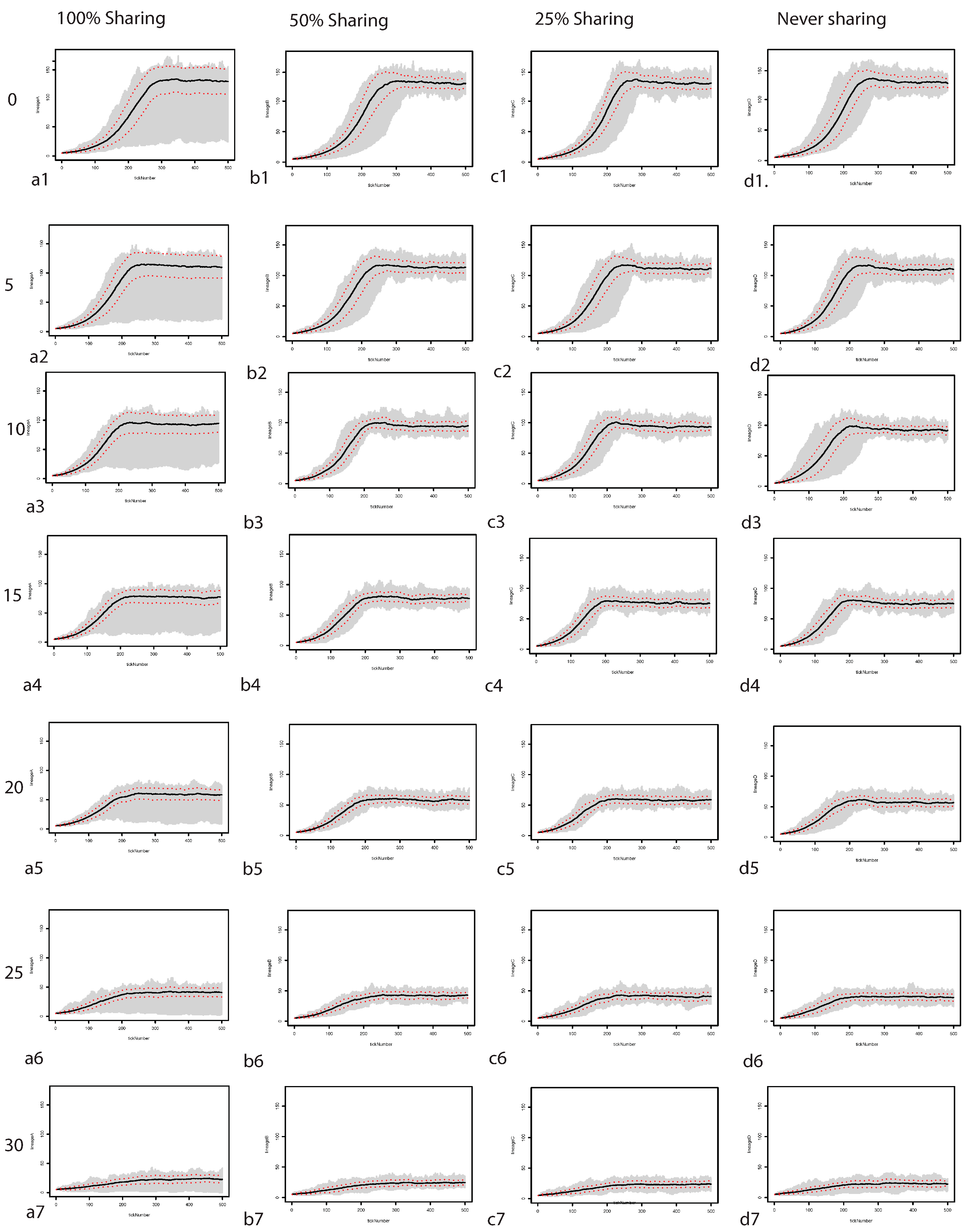
Figure 1.
Figure showing how each individual strategy responds to environmental pressures when no other lineage is present. Each tile is as follows: Columns marked A correspond to the 100% sharing strategy. Columns marked B correspond to the 50% sharing strategy. Columns marked C correspond to the 25% sharing strategy. Columns marked D correspond to 0% sharing strategy. Row 1 is 0% winter patch variability. Row 2 is 5% winter patch variability. Row 3 is 10% winter patch variability. Row 4 is 15% winter patch variability. Row 5 is 20% winter patch variability. Row 6 is 25% winter patch variability. Row 7 is 30% winter patch variability. Thus, tile c3 is the 25% sharing strategy under 10% patch variability. Y-axis goes from 0 to 150 households, X axis goes from 0 to 500 ticks. Red-dotted line corresponds to the standard deviation from the mean, while the gray lines show each strategy. Black central line corresponds to the mean of each strategy.
Hegmon [
6] found in her simulation of Hopi food sharing strategies that 100% cooperation was rarely the optimal strategy, but rather restricted sharing seemed to benefit the overall population the most. The results presented here compare positively with Hegmon’s findings. While the mean of each of the sharing strategies reported here is similar, the variance in the 100% sharing strategy suggests that sharing with no restrictions could be detrimental, even in favorable conditions. While the mean of the all-share strategy is similar to all the other strategies (
Figures S1–S7), the variance (
Figure 1) belies the fact that an all-share strategy could have highly unpredictable outcomes. The tighter variance around the mean in the other strategies suggests that those strategies would have more predictable outcomes.
Hegmon also suggests that hoarding (here represented at 0% sharing) is only a good option in the years of the worst productivity. When looking at graphs S1–S7 there appears to be no functional difference between any of the strategies, so this finding is not necessarily echoed in our results at this stage.
2.2. Multiple Strategies
Here we examine how populations respond to environmental stressors when each of the different strategies coexist in the same landscape. At the beginning of the simulation five agents of each strategy are seeded on the landscape. Experiments followed the same trajectory as above: with seven variables for patch variability and five random number seeds.
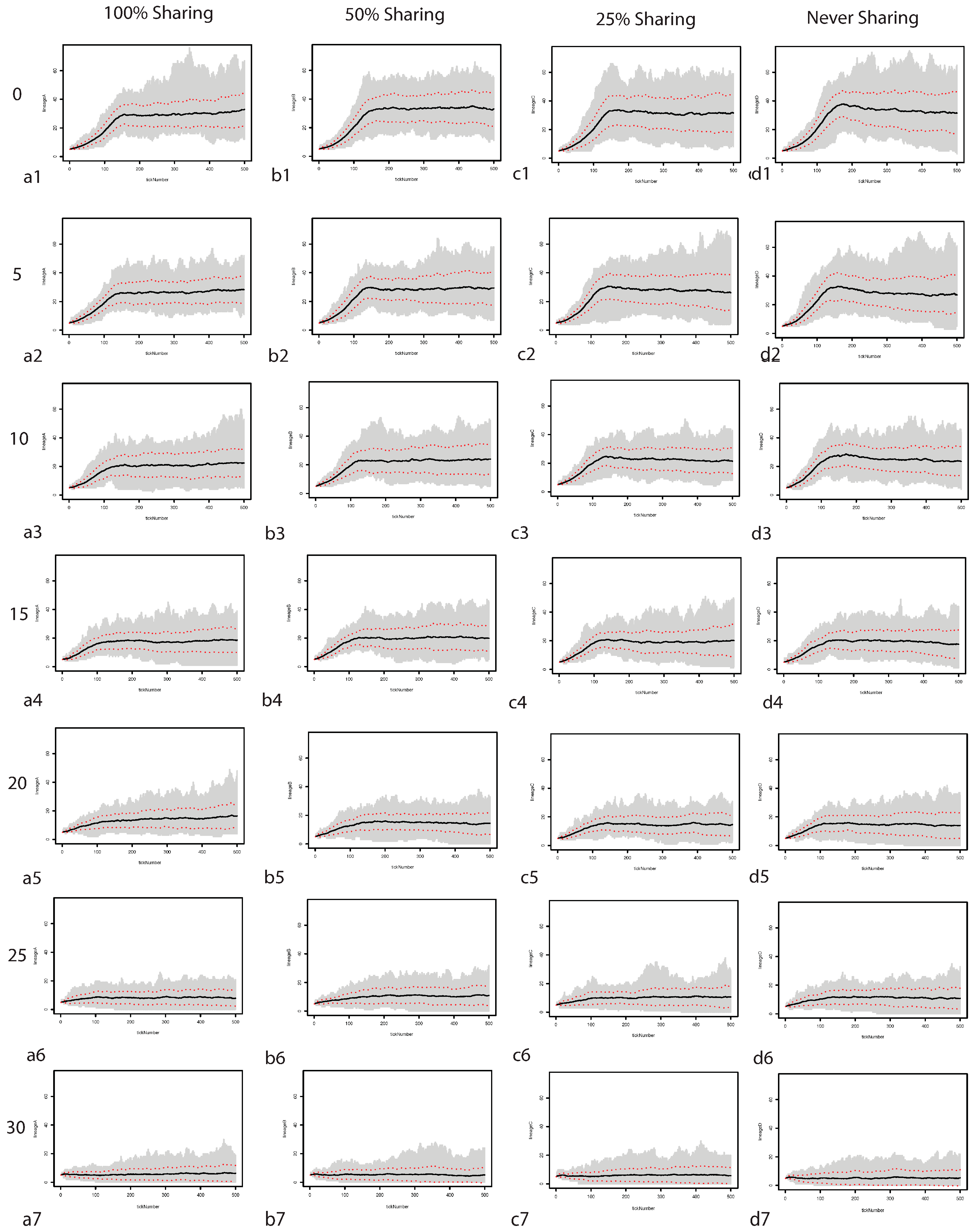
First of note is the scale: when only one strategy is represented the sum of that strategy is higher than the sum of that individual strategy when there are multiple strategies present. In
Figure 1 the scale is set to 150 agents, while in
Figure 2 the scale is set to 60 agents. Because of this, in
Figure 2 the variability might seem higher than it is when compared to
Figure 1, but variance around the mean is only ever approximately 40 agents in both
Figure 1 and
Figure 2 (
Figure 1 strategy A excluded).
Comparing the means of each strategy against one another on one graphic provides more helpful information. In
Figure 3,
Figure 4,
Figure 5,
Figure 6,
Figure 7,
Figure 8 and
Figure 9 each of the mean strategies are graphed on top of one another without the variance surrounding the mean as in
Figure 1 and
Figure 2. This allows us to directly compare the mean strategies without surrounding noise.
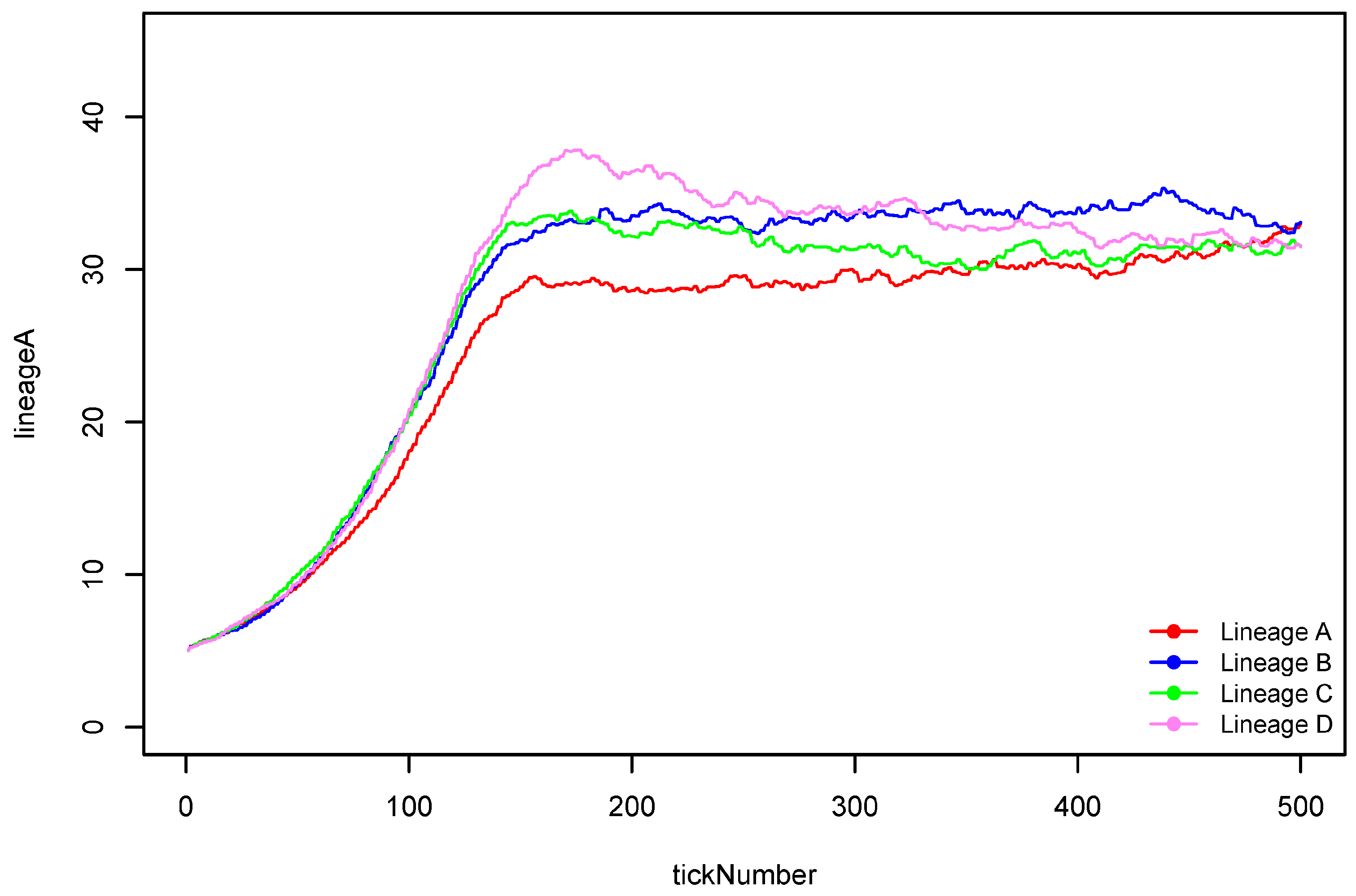
Figure 3 shows how each strategy fared against one another when the environment did not have any variability. To note, the 100% sharing strategy is never the best performing strategy. In these runs of the simulation, hoarding (0% sharing) is the highest performing strategy early in the simulation, while through time those
gers that subscribe to a hoarding strategy decrease in number. The strategy of sharing 50% of the time, however, is very stable, and eventually becomes the most populous strategy.
In a situation of stable population we may expect to see a convergence upon the mean as agents coalesce upon stable landscapes. A population under stress, however, will see a wide range of variation around the mean as agents attempt to maximize their resource acquisition while dealing with a volatile landscape (as seen above when only one strategy is represented). While the landscape in these runs of the simulation does not have year-to-year variability, the use of the land will create barren patches for five timesteps. Thus, early on gers that do not share do well on the landscape because there is little environmental impetus for sharing. With a predictable environment from year-to-year, independence can be a viable strategy. However, as the simulation progresses and gers create barren patches on the landscape from over-use, sharing can help gers avoid the variable productivity in the landscape they themselves have created.
Figure 2.
Figure showing how each individual strategy responds to environmental pressures when all other lineages are present. Each tile is as follows: Columns marked A correspond to the 100% sharing strategy. Columns marked B correspond to the 50% sharing strategy. Columns marked C correspond to the 25% sharing strategy. Columns marked D correspond to 0% sharing strategy. Row 1 is 0% winter patch variability. Row 2 is 5% winter patch variability. Row 3 is 10% winter patch variability. Row 4 is 15% winter patch variability. Row 5 is 20% winter patch variability. Row 6 is 25% winter patch variability. Row 7 is 30% winter patch variability. Thus, tile c3 is the 25% sharing strategy under 10% patch variability. Y-axis goes from 0 to 150 households, X-axis goes from 0 to 500 ticks. Red-dotted line corresponds to the standard deviation from the mean, while the gray lines show each strategy. Black central line corresponds to the mean of each strategy.
Figure 3.
Means of each of the strategies for 0% patch variability. Means correspond to Row 1 of
Figure 2. This figure reflects those runs when all strategies were present in the simulation.
Figure 3.
Means of each of the strategies for 0% patch variability. Means correspond to Row 1 of
Figure 2. This figure reflects those runs when all strategies were present in the simulation.
Figure 4.
Means of each of the strategies for 5% patch variability. Means correspond to Row 2 of
Figure 2. This figure reflects those runs when all strategies were present in the simulation.
Figure 4.
Means of each of the strategies for 5% patch variability. Means correspond to Row 2 of
Figure 2. This figure reflects those runs when all strategies were present in the simulation.
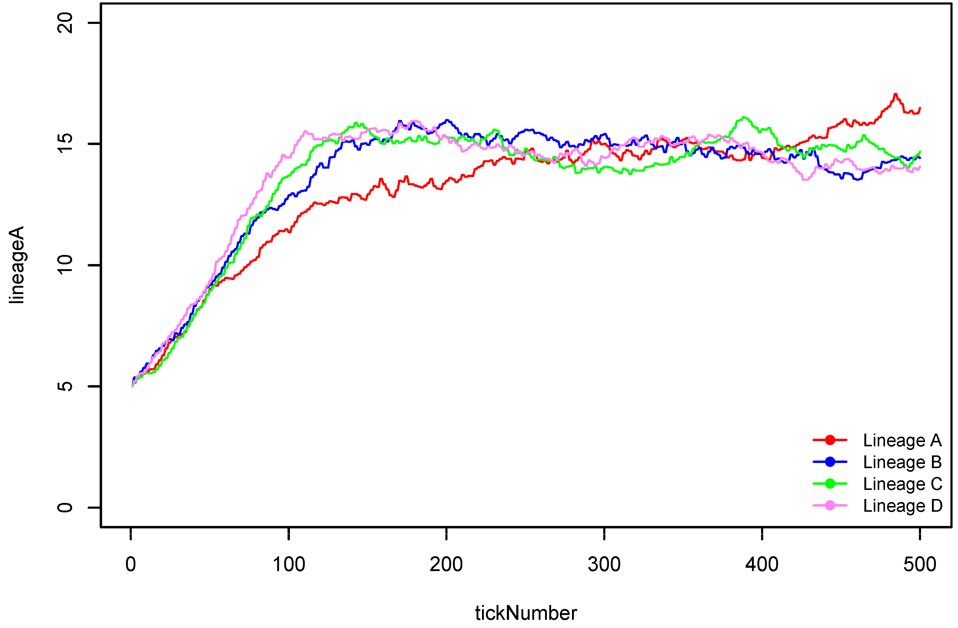
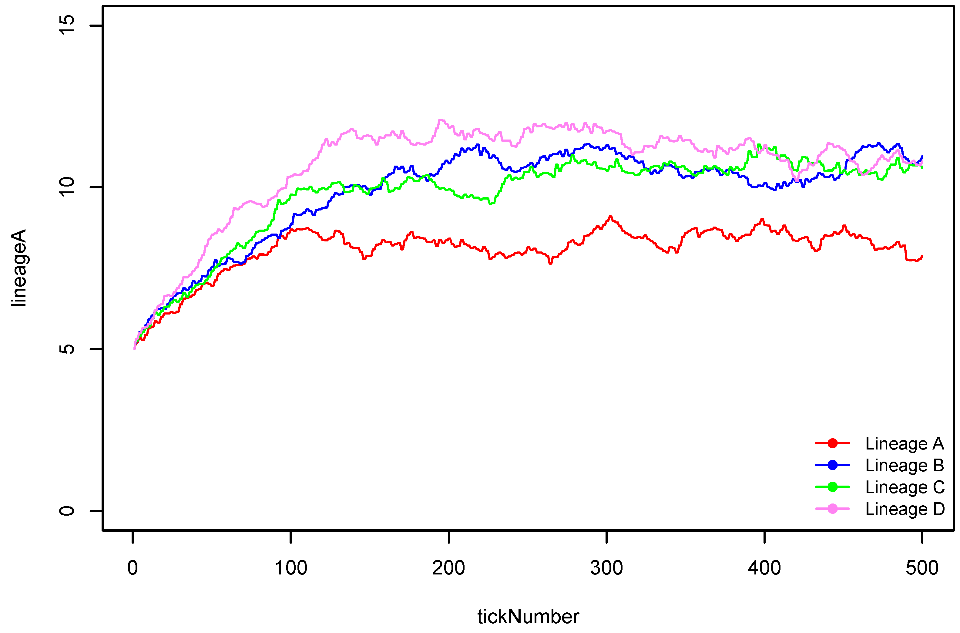
Figure 4 follows a similar trajectory to
Figure 3, with 100% sharing never being the best performing strategy of the four strategies, no sharing performing the best early on, and restricted sharing performing the best toward the end of the simulation.
Figure 5, however, begins to diverge from
Figure 3 and
Figure 4. In this figure the winter landscape had 10% variability. The sharing strategies are each fairly stable, reaching their own respective carrying capacities of 20 to 25 households on the landscape. In these runs of the simulation hoarding (0% sharing) is early on the highest performing strategy. However, this strategy has high variability, likely due to the unpredictability of the landscape, and the similar effect of overuse. However, as only 10% of the landscape is variable (due to the environment), independent
gers can make a living on the landscape with the simple rules created for this simulation.
Figure 5.
Means of each of the strategies for 10% patch variability. Means correspond to Row 3 of
Figure 2. This figure reflects those runs when all strategies were present in the simulation.
Figure 5.
Means of each of the strategies for 10% patch variability. Means correspond to Row 3 of
Figure 2. This figure reflects those runs when all strategies were present in the simulation.
Figure 6.
Means of each of the strategies for 15% patch variability. Means correspond to Row 4 of
Figure 2. This figure reflects those runs when all strategies were present in the simulation.
Figure 6.
Means of each of the strategies for 15% patch variability. Means correspond to Row 4 of
Figure 2. This figure reflects those runs when all strategies were present in the simulation.
Figure 7.
Means of each of the strategies for 20% patch variability. Means correspond to Row 5 of
Figure 2. This figure reflects those runs when all strategies were present in the simulation.
Figure 7.
Means of each of the strategies for 20% patch variability. Means correspond to Row 5 of
Figure 2. This figure reflects those runs when all strategies were present in the simulation.
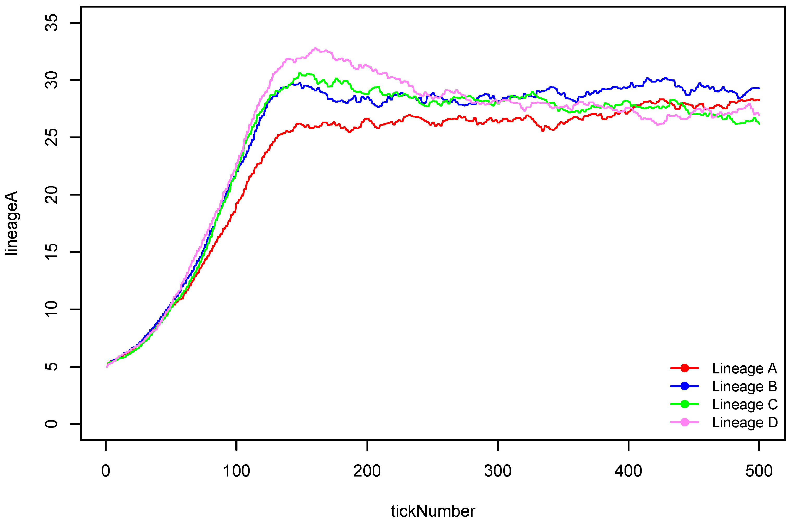
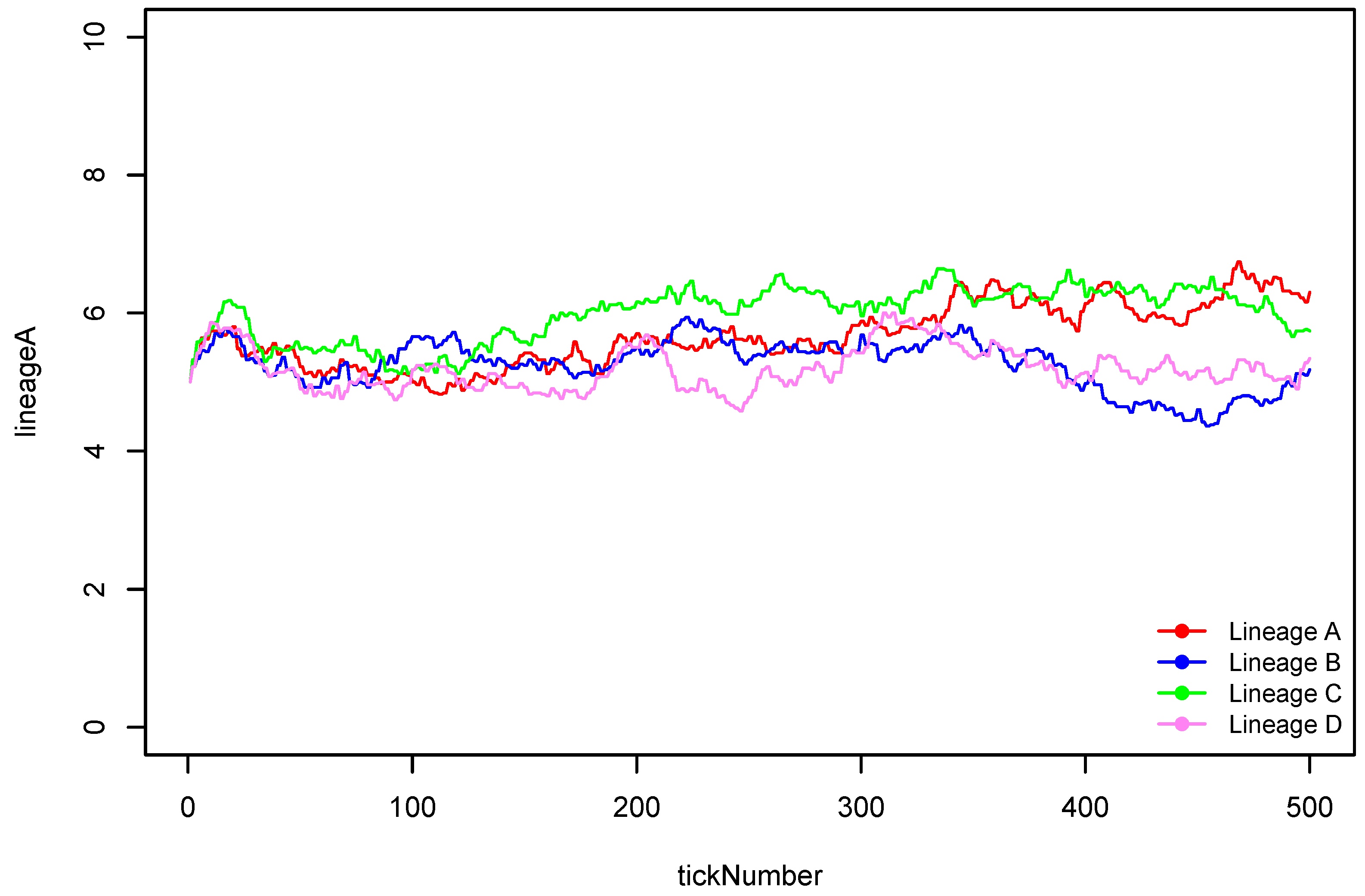
Once the environmental unpredictability of the landscape reaches 15%, hoarding is no longer the strategy with the highest population, and will only become optimal again when the landscape’s carrying capacity becomes very low (unpredictability of 25%). In
Figure 6 we can see that the means of the restricted sharing strategies (50% and 25% sharing) perform the best. Early in the simulation the 25% sharing strategy has the highest mean, while later in the simulation the 50% sharing strategy has the highest mean. This holds true for
Figure 7 as well. When the environmental landscape exhibits 20% unpredictability in winter patches, restricted sharing strategies perform well. Note, however, that in the final years of these simulations, the mean of the 100% sharing strategy performs well, while the other strategies remain relatively stable.
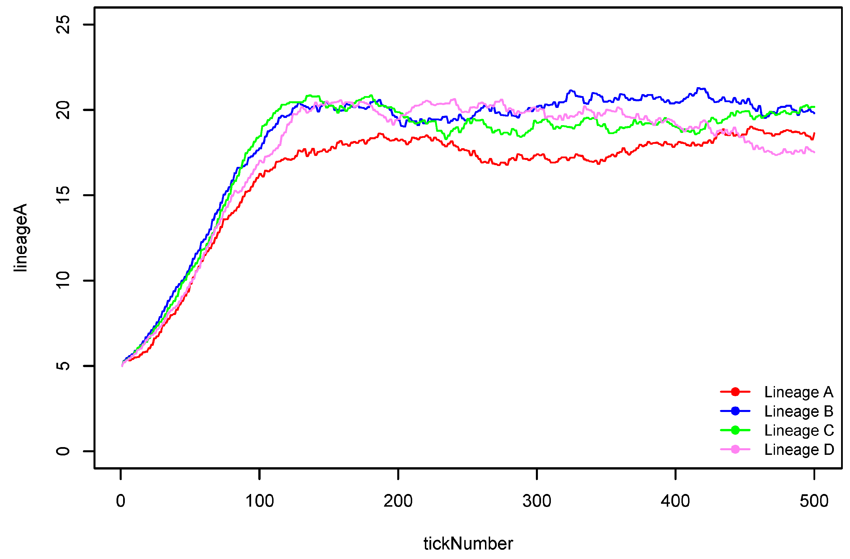
In
Figure 8 hoarding once again is the highest performing strategy. While above we suggest that hoarding is a good strategy when the landscape is productive enough that sharing is not necessary,
Figure 8 echoes Hegmon’s [
6] finding that hoarding is a viable strategy when the landscape is so poor that sharing will be detrimental for the overall population. Please note, however, that the difference in this graph between the restricted sharing strategies and the hoarding strategy is one household. In fact, many of the differences are rather small. Over the long term, however, even small differences in survivability (small adaptive advantages) may impact decision making.
In
Figure 9, when the landscape exhibits 30% unpredictability in winter patches, the averages of all of the four strategies are within one household. However, the 25% sharing strategy seems to have the highest mean on average. These results, when compared with
Figure 2(c7) show that this strategy also has the least variance (and thus might have the most predictable outcome).
Hegmon [
6] found in her simulations that the all-share strategy was never the optimal strategy, and that hoarding is an optimal strategy for a population when the environment is highly unpredictable. These findings are comparable to our study results, although we show that there is little necessity for sharing in a highly predictable landscape. Only when the landscape becomes changed due to use, or the environmental predictability becomes great, do sharing strategies become necessary.
Figure 8.
Means of each of the strategies for 25% patch variability. Means correspond to Row 6 of
Figure 2. This figure reflects those runs when all strategies were present in the simulation.
Figure 8.
Means of each of the strategies for 25% patch variability. Means correspond to Row 6 of
Figure 2. This figure reflects those runs when all strategies were present in the simulation.
Figure 9.
Means of each of the strategies for 30% patch variability. Means correspond to Row 7 of
Figure 2. This figure reflects those runs when all strategies were present in the simulation.
Figure 9.
Means of each of the strategies for 30% patch variability. Means correspond to Row 7 of
Figure 2. This figure reflects those runs when all strategies were present in the simulation.
Comparing
Figure 1 and
Figure 2 we can see that some similar patterns are apparent—an “all share” strategy never outperforms the other strategies, but there appears to be little functional difference among the other strategies. Each strategy reaches the logistic population curve (the carrying capacity) in
Figure 1, but in
Figure 2 there is greater variability. When comparing the means in
Figure 3,
Figure 4,
Figure 5,
Figure 6,
Figure 7,
Figure 8 and
Figure 9 we see that restricted sharing seems to be the most beneficial strategy when environmental conditions are unpredictable.
For a final means of comparison, we examined the statistical difference among the strategies with a Kolomgorov-Smirnov analysis. Kolomgorov-Smirnov analyses allow for direct comparability of each of the simulated means to see if there are statistical differences between each of the strategies. We simplified these data into five time slices: 100 ticks (50 years), 200 ticks (100 years), 300 ticks (150 years), 400 ticks (200 years), and 500 ticks (250 years). Further, we compared the pair-wise difference between the following means: Strategy A to Strategy B, Strategy B to Strategy C, Strategy C to Strategy D, and Strategy A to Strategy D.
Frequency differences as well as p-values to the 0.05 level are reported in
Table 3 and
Table 4.
Table 3 corresponds to
Figure 1 (single strategies modeled) while
Table 4 corresponds to
Figure 2 (all strategies present).
As can be seen in
Table 3, when only one lineage is represented, 31 of the 140 K-S statistic values show clear statistical significance in their difference. In
Table 4 we can see that 21 of the 140 values show clear statistical significance in their difference. Thus we can say that in 22% of the cases when only one lineage is represented there are real differences in the number of surviving households on the landscape, while when all lineages are represented 15% of the cases show real differences in the number of surviving households on the landscape. It is worth noting, the strongest difference is between strategy A (all share) and strategy D (no share) in both solo lineages and all lineages, with 17 and 11 cases showing statistical significance respectively. Little difference is seen in the restricted sharing strategies (50% and 25%) potentially showing that both of these are viable in most years and may be functionally the same.
In
Table 3, the highest and most significant variation seems to be related to reaching the environmental carrying capacity, which generally is reached between 100 and 200 ticks. Most other times variation is not significant except between extreme strategies in less variable landscapes. In
Table 4, however, variation is related to the end of the simulation, potentially showing that as sharing strategies stabilize the differences among them become more pronounced.
From
Figure 1 through
Figure 8 and
Table 3 and
Table 4 we may be able to interpret that during years of middling unpredictably, those households that do not freely share their resources with everyone (but do share with a select few) are likely to have their caloric needs met, are likely to reproduce, and are likely to survive into the next year. The significance in variation among the strategies suggests that there are real differences in all sharing, restricted sharing, and hoarding and, potentially, that individuals using those strategies would be able to see how well their strategy compared to other strategies. These findings are also echoed in Crabtree [
1]. Only during exceptional years would households want to horde their resources, potentially insuring their own survival at the detriment of others.
Table 3.
Results from Kolomgorov-Smirnov analysis on single lineage values. Data is simplified into five time slices: 100, 200, 300, 400 and 500 ticks. K-S values that show significance above a p-value of 0.05 are highlighted blue and show “Sig” in the significance column. This means that there is a large difference in the mean values for the lines during that tick for those variability values. Of note are the 17 K-S values that show as significant between Strategy A (all share) and Strategy D (no share).
| Tick | Variability | A to B Diff | p (0.05) | Sig? | B to C Diff | p (0.05) | Sig? | C to D Diff | p (0.05) | Sig? | A to D Diff | p (0.05) | Sig? |
|---|
| 100 | 0 | −0.0039 | 0.4643 | Not | 0.9322 | 0.4541 | Sig | 0.9450 | 0.4450 | Sig | 1.8733 | 0.4554 | Sig |
| 200 | 0 | 0.5399 | 0.2277 | Sig | 0.6984 | 0.2139 | Sig | 0.0349 | 0.2068 | Not | 1.2732 | 0.2210 | Sig |
| 300 | 0 | −0.0134 | 0.1683 | Not | −0.0834 | 0.1670 | Not | 0.0234 | 0.1673 | Not | −0.0735 | 0.1685 | Not |
| 400 | 0 | −0.0727 | 0.1686 | Not | −0.1445 | 0.1687 | Not | 0.0008 | 0.1698 | Not | −0.2164 | 0.1697 | Sig |
| 500 | 0 | −0.0786 | 0.1698 | Not | −0.0581 | 0.1690 | Not | −0.0617 | 0.1699 | Not | −0.1984 | 0.1707 | Sig |
| 100 | 5 | −0.3384 | 0.4049 | Not | 0.7353 | 0.4006 | Sig | 2.4859 | 0.3830 | Sig | 2.8827 | 0.3875 | Sig |
| 200 | 5 | 0.1088 | 0.1994 | Not | 0.1921 | 0.1951 | Not | 0.2645 | 0.1898 | Sig | 0.5654 | 0.1942 | Sig |
| 300 | 5 | −0.0642 | 0.1797 | Not | −0.0695 | 0.1801 | Not | −0.0898 | 0.1813 | Not | −0.2236 | 0.1809 | Sig |
| 400 | 5 | −0.0031 | 0.1819 | Not | −0.0457 | 0.1814 | Not | −0.1501 | 0.1830 | Not | −0.1989 | 0.1835 | Sig |
| 500 | 5 | 0.0090 | 0.1821 | Not | −0.0575 | 0.1815 | Not | −0.1158 | 0.1829 | Not | −0.1644 | 0.1834 | Not |
| 100 | 10 | −0.3478 | 0.3802 | Not | 0.3518 | 0.3787 | Not | 1.4646 | 0.3684 | Sig | 1.4686 | 0.3699 | Sig |
| 200 | 10 | 0.1627 | 0.2015 | Not | 0.0639 | 0.1981 | Not | −0.0319 | 0.1982 | Not | 0.1947 | 0.2017 | Not |
| 300 | 10 | −0.0182 | 0.1975 | Not | −0.0199 | 0.1972 | Not | −0.0402 | 0.1984 | Not | −0.0783 | 0.1987 | Not |
| 400 | 10 | −0.0318 | 0.1990 | Not | −0.0070 | 0.1987 | Not | −0.0108 | 0.1994 | Not | −0.0496 | 0.1997 | Not |
| 500 | 10 | −0.0758 | 0.1975 | Not | −0.0634 | 0.1984 | Not | −0.0421 | 0.2001 | Not | −0.1813 | 0.1992 | Not |
| 100 | 15 | 0.9795 | 0.3766 | Sig | 0.6125 | 0.3629 | Sig | 0.4403 | 0.3560 | Sig | 2.0323 | 0.3699 | Sig |
| 200 | 15 | 0.1259 | 0.2215 | Not | 0.1127 | 0.2175 | Not | 0.0984 | 0.2154 | Not | 0.3369 | 0.2195 | Sig |
| 300 | 15 | −0.0415 | 0.2173 | Not | −0.0891 | 0.2179 | Not | −0.0830 | 0.2208 | Not | −0.2136 | 0.2201 | Not |
| 400 | 15 | −0.0941 | 0.2185 | Not | −0.0195 | 0.2189 | Not | −0.0988 | 0.2211 | Not | −0.2124 | 0.2207 | Not |
| 500 | 15 | −0.0948 | 0.2189 | Not | −0.0888 | 0.2202 | Not | 0.0077 | 0.2219 | Not | −0.1758 | 0.2206 | Not |
| 100 | 20 | 1.1205 | 0.4076 | Sig | 0.3596 | 0.3919 | Not | 0.0860 | 0.3871 | Not | 1.5661 | 0.4030 | Sig |
| 200 | 20 | 0.2353 | 0.2575 | Not | 0.0125 | 0.2525 | Not | 0.1005 | 0.2504 | Not | 0.3484 | 0.2554 | Sig |
| 300 | 20 | −0.0510 | 0.2490 | Not | −0.1482 | 0.2504 | Not | −0.0548 | 0.2529 | Not | −0.2540 | 0.2515 | Sig |
| 400 | 20 | −0.2497 | 0.2539 | Not | 0.0424 | 0.2554 | Not | 0.0390 | 0.2538 | Not | −0.1684 | 0.2523 | Not |
| 500 | 20 | −0.0855 | 0.2531 | Not | 0.0381 | 0.2523 | Not | −0.1037 | 0.2528 | Not | −0.1511 | 0.2536 | Not |
| 100 | 25 | 0.1657 | 0.4510 | Not | 0.0865 | 0.4458 | Not | 0.9166 | 0.4370 | Sig | 1.1688 | 0.4422 | Sig |
| 200 | 25 | −0.0232 | 0.3144 | Not | 0.1499 | 0.3108 | Not | 0.0877 | 0.3089 | Not | 0.2144 | 0.3125 | Not |
| 300 | 25 | 0.0601 | 0.2992 | Not | 0.0379 | 0.2960 | Not | −0.2026 | 0.3007 | Not | −0.1046 | 0.3039 | Not |
| 400 | 25 | −0.1161 | 0.2979 | Not | −0.0560 | 0.2994 | Not | 0.0682 | 0.3011 | Not | −0.1039 | 0.2996 | Not |
| 500 | 25 | 0.0443 | 0.2981 | Not | −0.1278 | 0.2980 | Not | −0.1582 | 0.3048 | Not | −0.2418 | 0.3048 | Not |
| 100 | 30 | 0.4897 | 0.5757 | Not | 0.1157 | 0.5568 | Not | 0.6519 | 0.5490 | Sig | 1.2573 | 0.5681 | Sig |
| 200 | 30 | 0.3456 | 0.4389 | Not | 0.0173 | 0.4243 | Not | 0.1977 | 0.4234 | Not | 0.5606 | 0.4380 | Sig |
| 300 | 30 | −0.1855 | 0.4030 | Not | 0.1829 | 0.3969 | Not | −0.2921 | 0.4030 | Not | −0.2946 | 0.4089 | Not |
| 400 | 30 | −0.2528 | 0.3964 | Not | −0.0964 | 0.3984 | Not | 0.1441 | 0.4008 | Not | −0.2051 | 0.3988 | Not |
| 500 | 30 | 0.0848 | 0.3964 | Not | −0.1236 | 0.3911 | Not | −0.2040 | 0.4021 | Not | −0.2429 | 0.4073 | Not |
Table 4.
Results from Kolomgorov-Smirnov analysis on multiple present lineage values. Data is simplified into five time slices: 100, 200, 300, 400 and 500 ticks. K-S values that show significance above a p-value of 0.05 are highlighted blue and show “Sig” in the significance column. This means that there is a large difference in the mean values for the lines during that tick for those variability values. Of note are the 11 K-S values that show as significant between Strategy A (all share) and Strategy D (no share).
| Tick | Variability | A to B Diff | p (0.05) | Sig? | B to C Diff | p (0.05) | Sig? | C to D Diff | p (0.05) | Sig? | A to D Diff | p (0.05) | Sig? |
|---|
| 100 | 0 | 0.2004 | 0.4380 | Not | 0.3571 | 0.4245 | Not | −0.2796 | 0.4234 | Not | 0.2779 | 0.4369 | Not |
| 200 | 0 | 0.2692 | 0.3461 | Not | 0.0617 | 0.3356 | Not | 0.3047 | 0.3290 | Not | 0.6357 | 0.3397 | Sig |
| 300 | 0 | 0.0921 | 0.3421 | Not | −0.0769 | 0.3376 | Not | 0.0921 | 0.3374 | Not | 0.1073 | 0.3418 | Not |
| 400 | 0 | 0.0600 | 0.3396 | Not | −0.1675 | 0.3375 | Not | −0.0582 | 0.3414 | Not | −0.1657 | 0.3435 | Not |
| 500 | 0 | −0.4464 | 0.3346 | Sig | 0.0393 | 0.3384 | Not | −0.2786 | 0.3426 | Not | −0.6857 | 0.3388 | Sig |
| 100 | 5 | 0.3933 | 0.4242 | Not | 0.2278 | 0.4091 | Not | 0.0064 | 0.4060 | Not | 0.6275 | 0.4212 | Sig |
| 200 | 5 | −0.0263 | 0.3664 | Not | 0.1897 | 0.3594 | Not | 0.2578 | 0.3515 | Not | 0.4212 | 0.3587 | Sig |
| 300 | 5 | −0.0153 | 0.3687 | Not | 0.1085 | 0.3630 | Not | −0.1126 | 0.3637 | Not | −0.0193 | 0.3694 | Not |
| 400 | 5 | 0.0124 | 0.3617 | Not | −0.0632 | 0.3588 | Not | −0.2068 | 0.3645 | Not | −0.2577 | 0.3673 | Not |
| 500 | 5 | −0.1759 | 0.3586 | Not | −0.3916 | 0.3658 | Sig | 0.0195 | 0.3732 | Not | −0.5480 | 0.3662 | Sig |
| 100 | 10 | 0.2237 | 0.4490 | Not | 0.2567 | 0.4320 | Not | 0.0896 | 0.4148 | Not | 0.5700 | 0.4324 | Sig |
| 200 | 10 | 0.0212 | 0.4163 | Not | 0.2597 | 0.4034 | Not | 0.2083 | 0.3841 | Not | 0.4891 | 0.3976 | Sig |
| 300 | 10 | 0.0690 | 0.4135 | Not | 0.1053 | 0.4029 | Not | −0.1896 | 0.3943 | Not | −0.0153 | 0.4051 | Not |
| 400 | 10 | −0.1458 | 0.4068 | Not | −0.1439 | 0.4062 | Not | 0.0799 | 0.3974 | Not | −0.2098 | 0.3979 | Not |
| 500 | 10 | −0.0832 | 0.3995 | Not | −0.4201 | 0.4036 | Sig | −0.2177 | 0.4058 | Not | −0.7211 | 0.4017 | Sig |
| 100 | 15 | −0.0535 | 0.4671 | Not | 0.2600 | 0.4522 | Not | −0.2272 | 0.4570 | Not | −0.0206 | 0.4718 | Not |
| 200 | 15 | −0.1695 | 0.4438 | Not | 0.1588 | 0.4341 | Not | 0.0890 | 0.4338 | Not | 0.0783 | 0.4435 | Not |
| 300 | 15 | 0.2532 | 0.4448 | Not | −0.1974 | 0.4332 | Not | 0.3611 | 0.4346 | Not | 0.4169 | 0.4462 | Not |
| 400 | 15 | 0.1459 | 0.4397 | Not | −0.3176 | 0.4334 | Not | 0.2244 | 0.4405 | Not | 0.0528 | 0.4468 | Not |
| 500 | 15 | −0.1826 | 0.4389 | Not | 0.1344 | 0.4302 | Not | −0.5178 | 0.4441 | Sig | −0.5659 | 0.4525 | Sig |
| 100 | 20 | 0.5377 | 0.5536 | Not | 0.3391 | 0.5278 | Not | 0.3074 | 0.5129 | Not | 1.1842 | 0.5394 | Sig |
| 200 | 20 | 0.6620 | 0.5029 | Sig | −0.2177 | 0.4868 | Not | 0.0377 | 0.4922 | Not | 0.4821 | 0.5082 | Not |
| 300 | 20 | −0.0424 | 0.4934 | Not | −0.4549 | 0.5017 | Not | 0.1634 | 0.5097 | Not | −0.3339 | 0.5016 | Not |
| 400 | 20 | −0.1135 | 0.5049 | Not | 0.3205 | 0.4952 | Not | −0.2821 | 0.4951 | Not | −0.0752 | 0.5048 | Not |
| 500 | 20 | −0.7894 | 0.4904 | Sig | 0.0886 | 0.5042 | Not | −0.1860 | 0.5075 | Not | −0.8868 | 0.4937 | Sig |
| 100 | 25 | −0.9495 | 0.6491 | Sig | 0.5460 | 0.6308 | Not | −0.0947 | 0.6066 | Not | −0.4983 | 0.6257 | Not |
| 200 | 25 | 0.2414 | 0.6260 | Not | −0.3957 | 0.5986 | Not | 0.5060 | 0.5851 | Not | 0.3517 | 0.6131 | Not |
| 300 | 25 | 0.1750 | 0.6084 | Not | −0.3469 | 0.5827 | Not | 0.1769 | 0.5774 | Not | 0.0051 | 0.6033 | Not |
| 400 | 25 | −0.2866 | 0.6258 | Not | 0.4883 | 0.5893 | Not | −0.3176 | 0.5732 | Not | −0.1159 | 0.6107 | Not |
| 500 | 25 | 0.6869 | 0.6352 | Sig | −0.1668 | 0.5859 | Not | −0.2757 | 0.5880 | Not | 0.2444 | 0.6372 | Not |
| 100 | 30 | 1.0337 | 0.8347 | Sig | −0.8822 | 0.8270 | Sig | 0.5212 | 0.8451 | Not | 0.6727 | 0.8526 | Not |
| 200 | 30 | 0.1821 | 0.8129 | Not | 0.1558 | 0.7978 | Not | −0.0795 | 0.7978 | Not | 0.2585 | 0.8129 | Not |
| 300 | 30 | 0.1819 | 0.8001 | Not | −0.1592 | 0.7975 | Not | 0.0087 | 0.8072 | Not | 0.0313 | 0.8098 | Not |
| 400 | 30 | −0.6953 | 0.8201 | Not | 0.7294 | 0.8172 | Not | −0.4789 | 0.8101 | Not | −0.4448 | 0.8131 | Not |
| 500 | 30 | −0.6060 | 0.8066 | Not | 0.1113 | 0.8242 | Not | 0.1235 | 0.8177 | Not | −0.3712 | 0.8000 | Not |
2.3. Discussion
Winterhalder and Leslie [
32] have shown that long-term stochastic processes may affect how individuals react to environmental conditions and how they approach risk. In their model, demographic response to an unpredictable environment will, by nature, be nonlinear. For example, people cannot predict exactly how many children to have so that four children will grow into adulthood. The results of our above analysis echo those of Winterhalder and Leslie and show that individuals may indeed seek risk when environments are highly unstable in order to have the chance of surviving, and may be risk-averse when environments are stable. The high levels of variance observed in the model presented in this paper are at least partially reflective of the unpredictable, highly unstable environments in which this simulation occurs. While Hegmon [
6] found that restricted sharing will be the most beneficial strategy for overall populations (restricted sharing should decrease variance), Winterhalder and Leslie’s findings may highlight why highly variance will be beneficial in unpredictable environments. People may need to try multiple strategies to survive.
Powers and Lehman [
2] found that sharing increases the carrying capacity of a system. Such a result is potentially visible in our results as well. When environmental pressures become great, and households group together, the environmental pressures can become mitigated by the social sharing strategy. However, despite sharing strategies lessening environmental pressures, households are never outside of those environmental pressures, and the use of the landscape creates environmental pressures as well due to patch degradation.
Pastoralists have long been blamed for environmental degradation from overgrazing [
33]. The “tragedy of the commons” theory states that unmonitored common-pool resources, as is the case in Mongolia with individual ownership of herds, but not land, leads to irresponsible usage of resources. However, critics of this theory point to various formal and informal social adaptations that oversee and regulate resource use [
34]. The same cooperation and sharing networks modeled here may parallel the social networks ensuring sustainable resource utilization through traditional ecological knowledge.
The problem of common-pool resources is evident in the model. When agents land on patches they extract the resources from those patches, and must wait multiple timesteps until those patches regenerate. It is possible that all winter patches in one area could become used during one timestep, causing future households to have no opportunities for productive patches. If agents land on dead patches they are charged energy. Once agents have fewer than 10 energy stored, those agents with a sharing strategy must rely on other agents in their network for survival. In this way we can see how agents react to a simulated tragedy of the commons. Once resources are over-exploited in an area, households must call upon their networks for help. As we see in this simulation, agents are doubly burdened by both simulated dzuds and by simulated resource over-use. Those agents that are able to rely on their greater social network fare better overall than those agents with no social network when both climatic and overuse pressures affect the environment.
One final issue addressed by this model is the poor resolution of the archaeological record. While research is ongoing in household studies in Mongolia (e.g., [
12]) most studies in Mongolia have focused on monumental archaeology. This is coupled with poor resolution of household archaeology (centimeters of deposition equating to centuries of occupation). Consequently, our understanding of the past can be blurred. Simulations, therefore, help us to address these gaps in our knowledge.
Notably missing from our study is a goodness-of-fit exercise between the model and the real settlement patterns [
1,
35]. This is due in part to there not being many complete archaeological datasets in the region to do goodness-of-fit tests against yet. Consequently, we must make do and use models as a way to inform our understanding of the limited archaeological information available at this time.
This model, while not meant as a reproduction of reality, presents a plausible scenario based on developed theory and hopes to address key questions of how semi-nomadic Mongolians address local weather events, such as drought and heavy winters. While this model is highly simplified, it presents a plausible suite of directions that people in this highly unpredictable environment could face. Therefore the outcome of our study can be used to make some conclusions of a much more complicated system.


