Development of Future Land Cover Change Scenarios in the Metropolitan Fringe, Oregon, U.S., with Stakeholder Involvement


Abstract
:1. Introduction
2. Methods
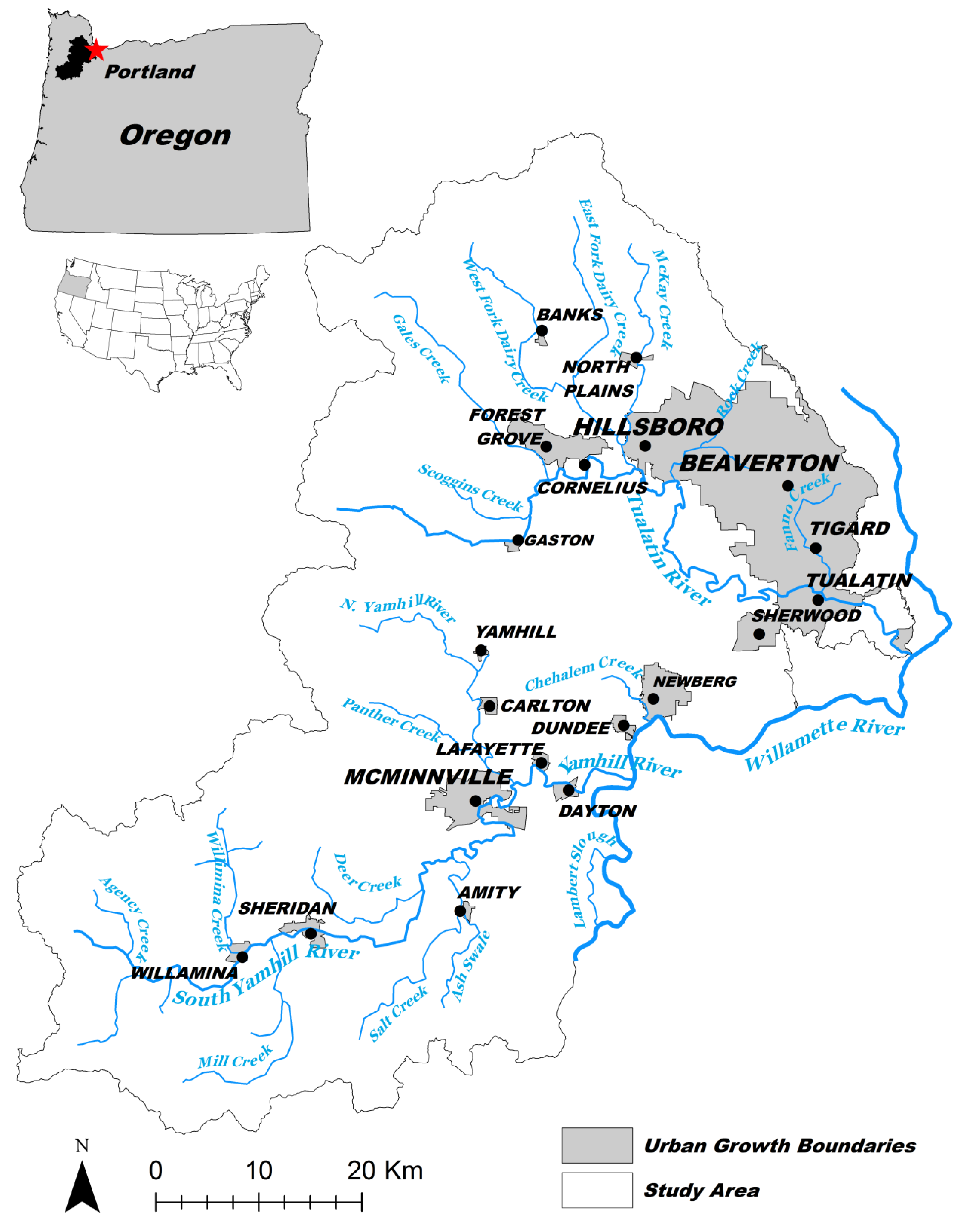
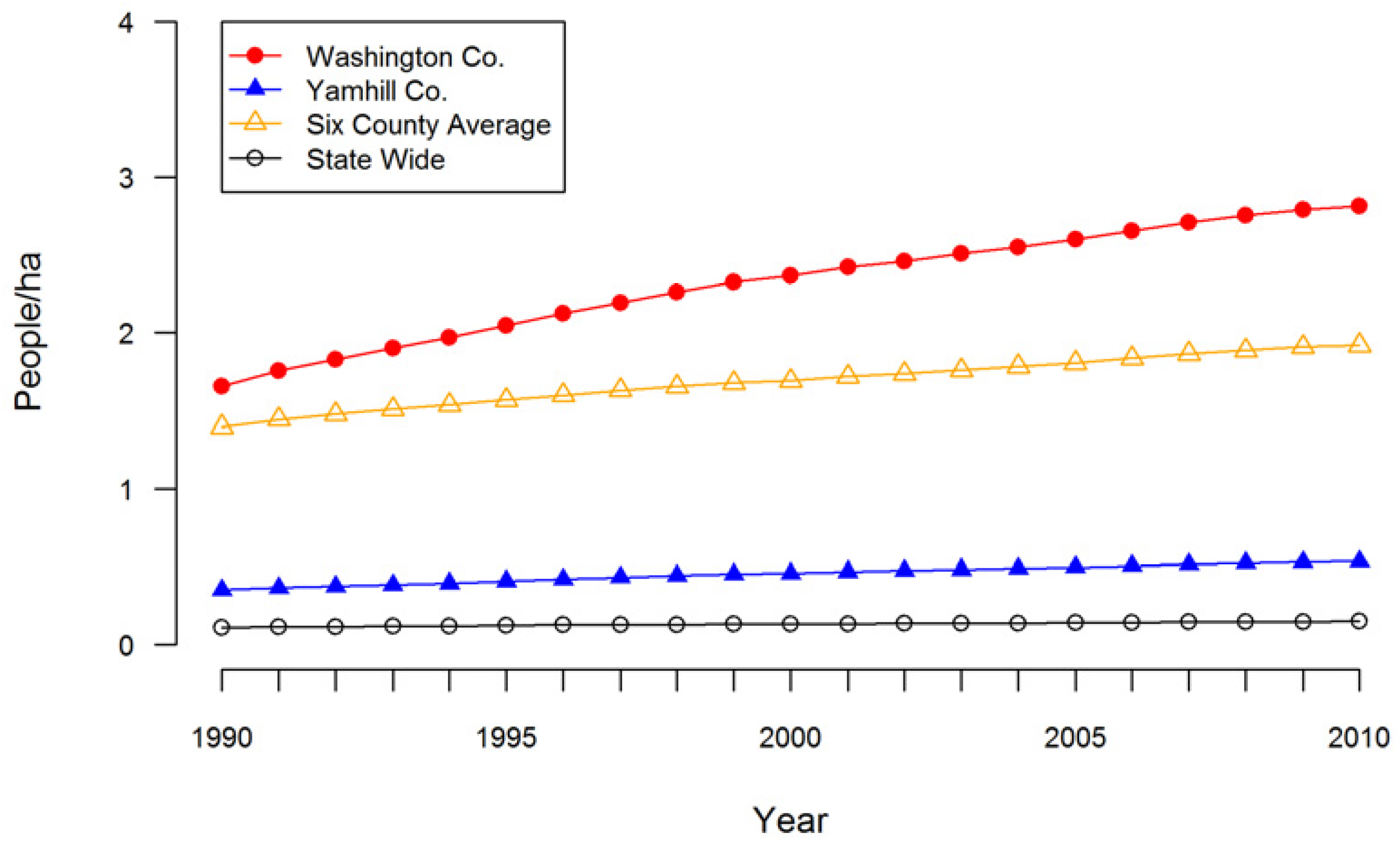
2.1. Study Area

| Pop. 1980 | Pop. 1990 | Pop. 2000 | Pop. 2010 | Ann. Ave. Change | Total Change | |
|---|---|---|---|---|---|---|
| County | ||||||
| Washington | 245,860 | 311,554 | 445,342 | 529,710 | 2.39% | 115.4% |
| Yamhill | 55,332 | 65,551 | 84,992 | 99,193 | 1.90% | 79.3% |
| Large Cities | ||||||
| Beaverton | 31,962 | 53,307 | 76,129 | 89,803 | 3.39% | 181.0% |
| Hillsboro | 27,664 | 37,598 | 70,186 | 91,611 | 3.94% | 223.2% |
| McMinnville | 14,080 | 17,894 | 26,499 | 32,187 | 2.70% | 128.6% |
| Newberg | 10,394 | 13,086 | 18,064 | 22,068 | 2.46% | 112.3% |


| 1992 to 2001 Urban Change (ha) | Percent Change | 2001 to 2006 Urban Change (ha) | Percent Change | |
|---|---|---|---|---|
| County | ||||
| Washington | 1209 | 4.3% | 1073 | 3.0% |
| Yamhill | 260 | 20.8% | 381 | 3.0% |
| Large Cities | ||||
| Beaverton | 108 | 2.5% | 43 | 1.0% |
| Hillsboro | 293 | 6.5% | 288 | 5.8% |
| McMinnville | 34 | 1.8% | 138 | 7.2% |
| Newberg | 89 | 8.1% | 43 | 10.9% |
| Study Area | 1669 | 3.1% | 1476 | 2.7% |
2.2. Data
| Data Type | Description | Sources |
|---|---|---|
| Urban Growth Boundaries (UGB) | Includes current UGB plus accepted and proposed urban reserve areas (URAs), rural reserves with additional protection and some additional adjacent land in case growth exceeds current reserves. | Metro Regional Land and Information System (RLIS), City of McMinnville Planning Department, City of Newberg Engineering Department |
| Zoning | Includes all except a few small communities. A statewide layer designating broad classifications (forestry, agriculture and rural residential) was integrated with municipality zoning layers. | RLIS, Mid-Willamette Valley Council of Governments (City of Dayton’s zoning estimated from online map) |
| Measure 49 Claims | 632 claims joined to tax lot parcel data to make spatially explicit. Authorized claims collected from three counties making up the vast majority of the study area. | Oregon Department of Land Conservation and Development, State of Oregon Geospatial Enterprise Office, Yamhill County Assessor’s Office |
| High Value Farm Soils | Agriculture soils of U.S. Natural Resource Conservation Service Class I and II (irrigated or non-irrigated) | Oregon Spatial Library |
| Groundwater Restriction Zones | Critical and restricted groundwater zones could possibly be an impediment to rural residential development. Designated by the Oregon Department of Water Resources where aquifers are identified as depleted or used at an unsustainable rate | Oregon Department of Water Resources |
| Protected Areas | Lands off-limits to development for a variety of reasons, including federal forest lands, city and state parks, private green spaces and schools. | RLIS, U.S. Fish Wildlife Geospatial Services |
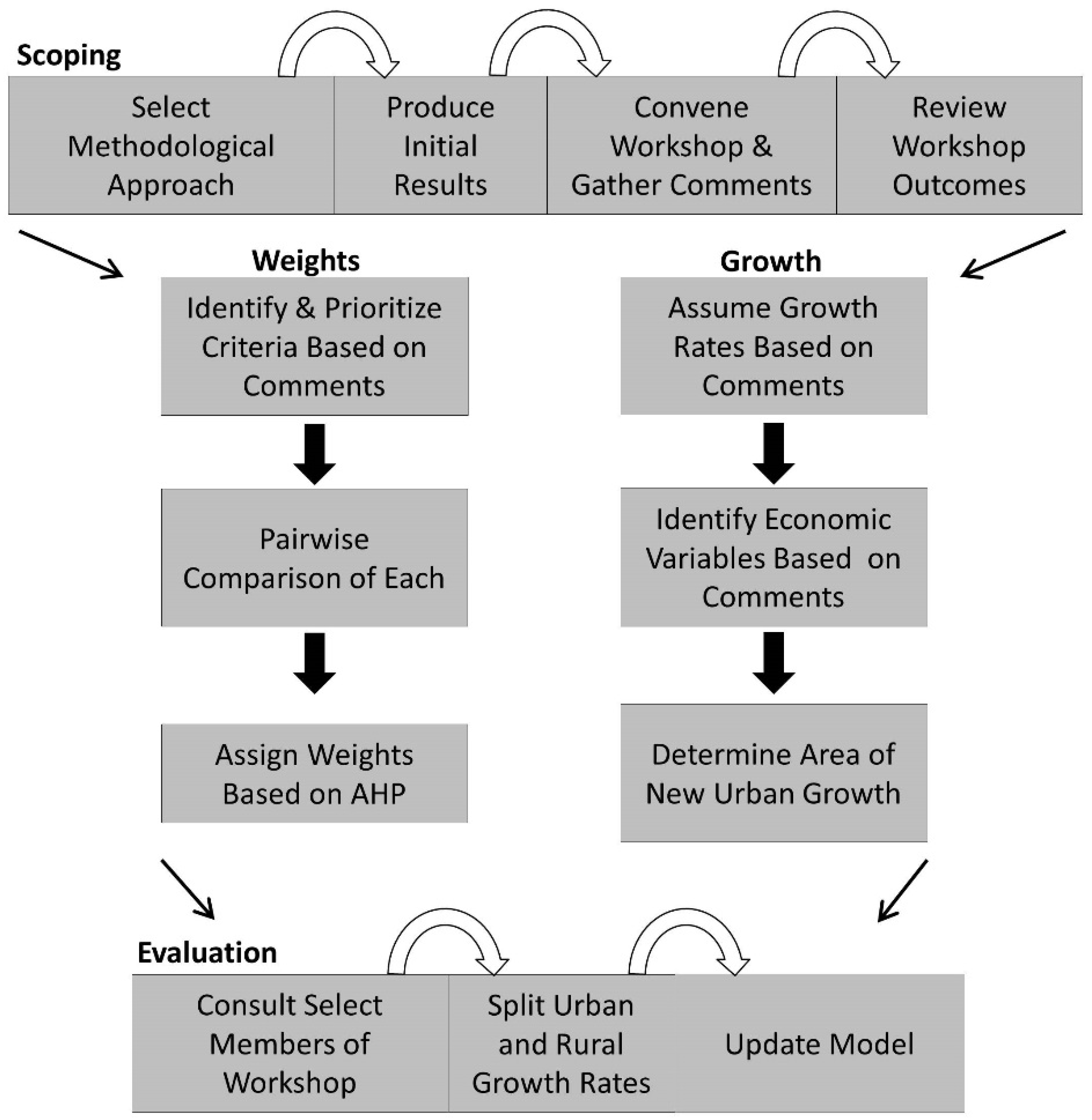
2.3. Construction of Scenarios with Stakeholder Consultation
| Scenario | Area | Ann. Pop. Growth | Future Jobs per Ha | Total Jobs per Ha | Future Households per Ha | Total Households per Ha |
|---|---|---|---|---|---|---|
| Current (NLCD 2006) | Urban | 82.4 | 8.8 | |||
| Current (NLCD 2006) | Rural | 95.3 | 3.2 | |||
| Future Low | Urban | 0.57% | 86.5 | 83.5 | 42.0 | 10.4 |
| Future Low | Rural | 0.03% | 96.4 | 95.4 | 6.2 | 3.2 |
| Future Medium | Urban | 1.43% | 86.5 | 84.3 | 42.0 | 13.3 |
| Future Medium | Rural | 0.08% | 96.4 | 95.4 | 6.2 | 3.2 |
| Future High | Urban | 1.90% | 86.5 | 84.7 | 42.0 | 14.4 |
| Future High | Rural | 0.10% | 96.4 | 95.4 | 6.2 | 3.3 |
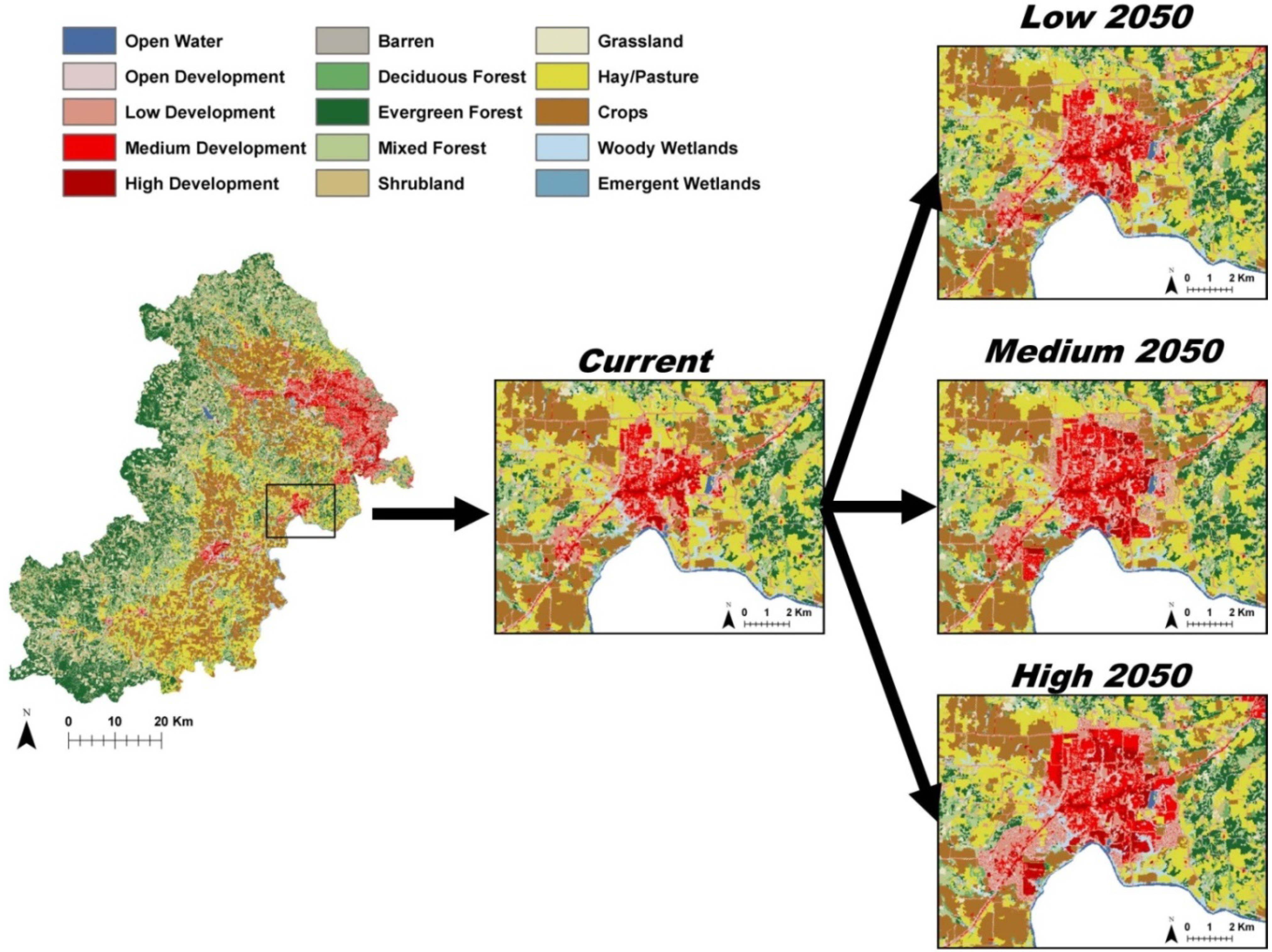
| Scenario | High Dev. | Medium Dev. | Low Dev. | Open Dev. | |
|---|---|---|---|---|---|
| Low | Urban | 1250 (37%) | 603 (5%) | 944 (5%) | 260 (5%) |
| Rural | 34 (12%) | 5 (1%) | 40 (1%) | 64 (1%) | |
| Medium | Urban | 3046 (91%) | 1805 (16%) | 2823 (16%) | 777 (2%) |
| Rural | 41 (14%) | 13 (2%) | 108 (4%) | 173 (2%) | |
| High | Urban | 4331 (129%) | 2665 (24%) | 4168 (23%) | 1148 (23%) |
| Rural | 44 (15%) | 18 (2%) | 146 (2%) | 234 (4%) |
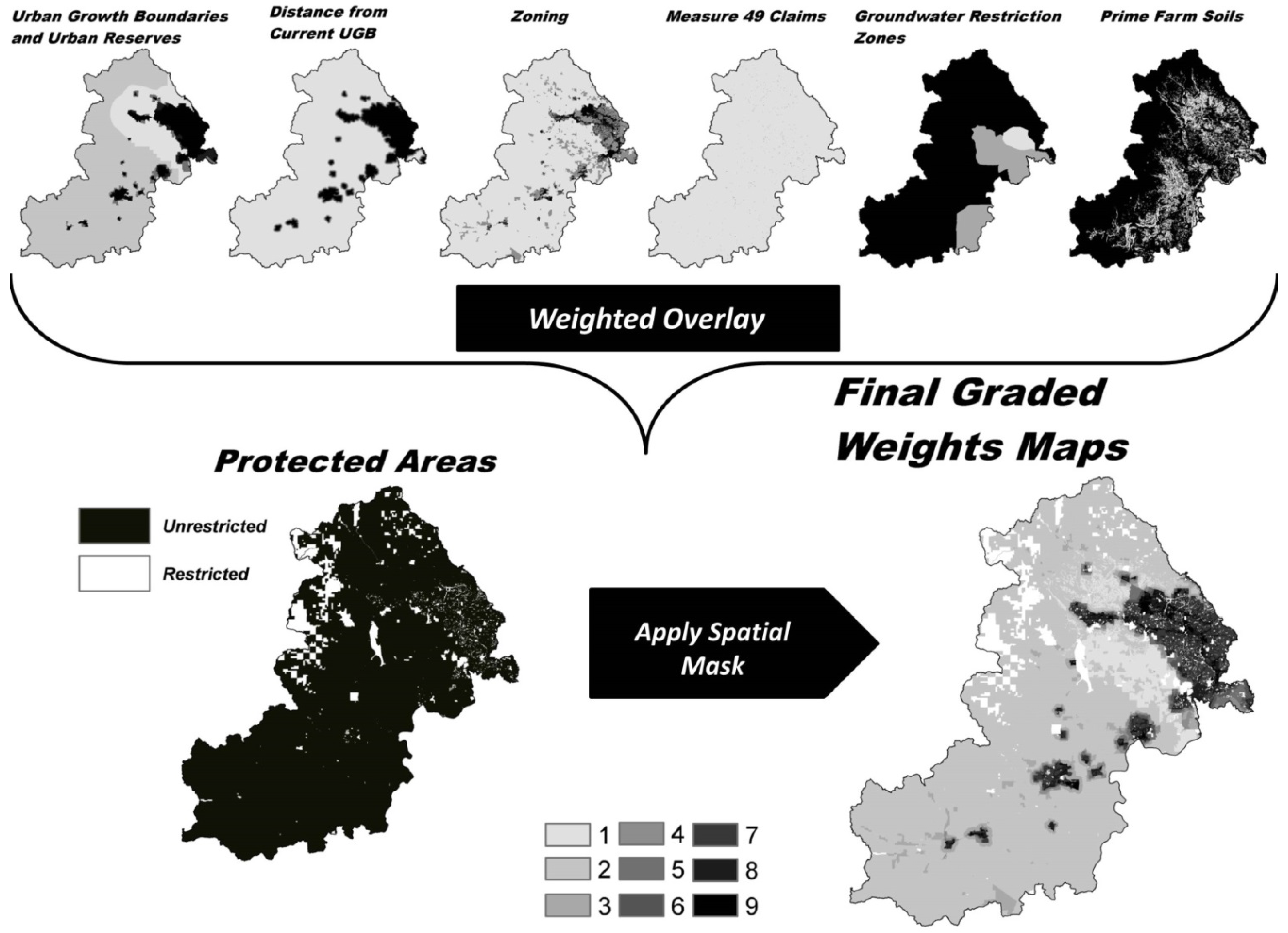
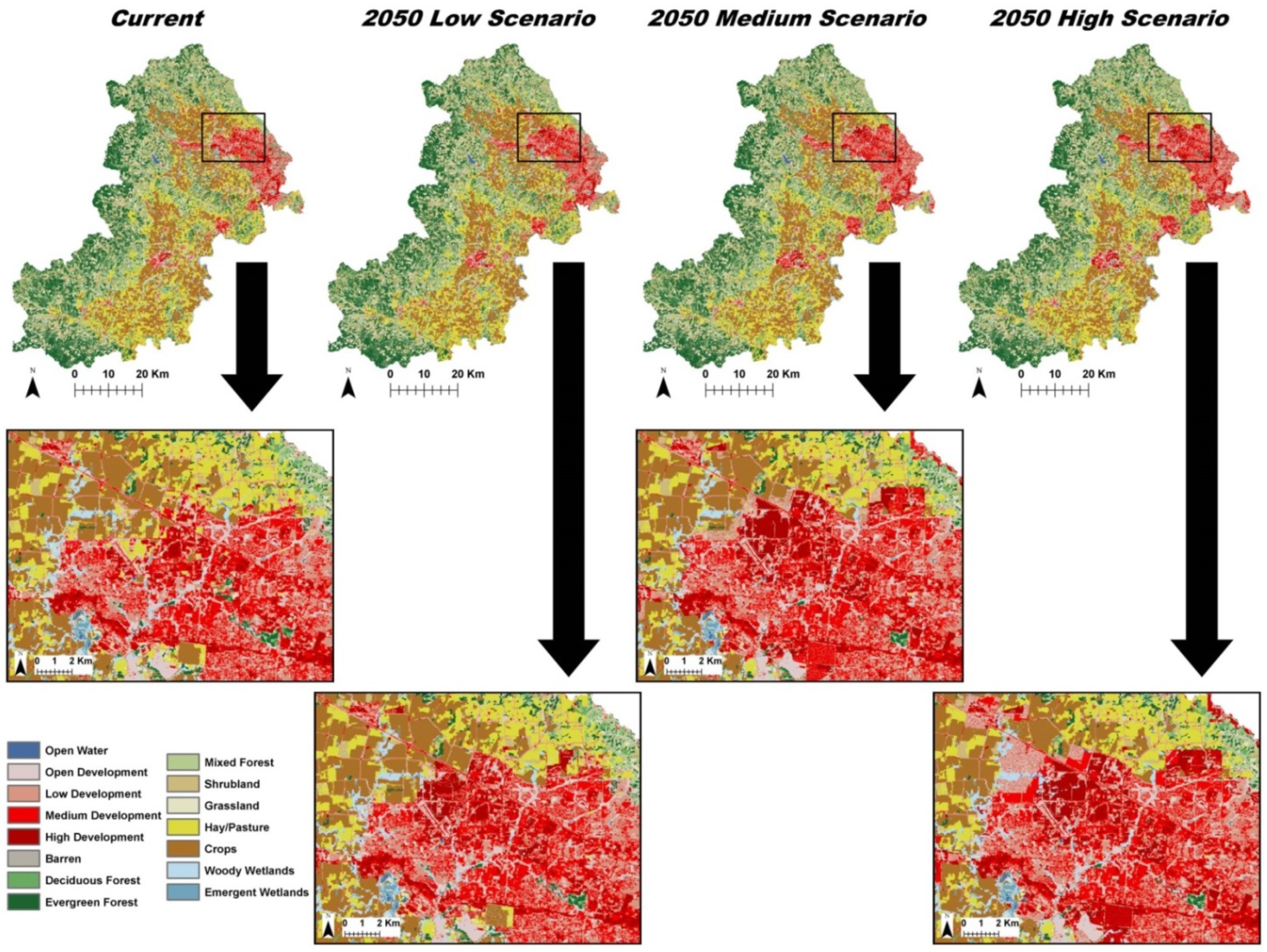
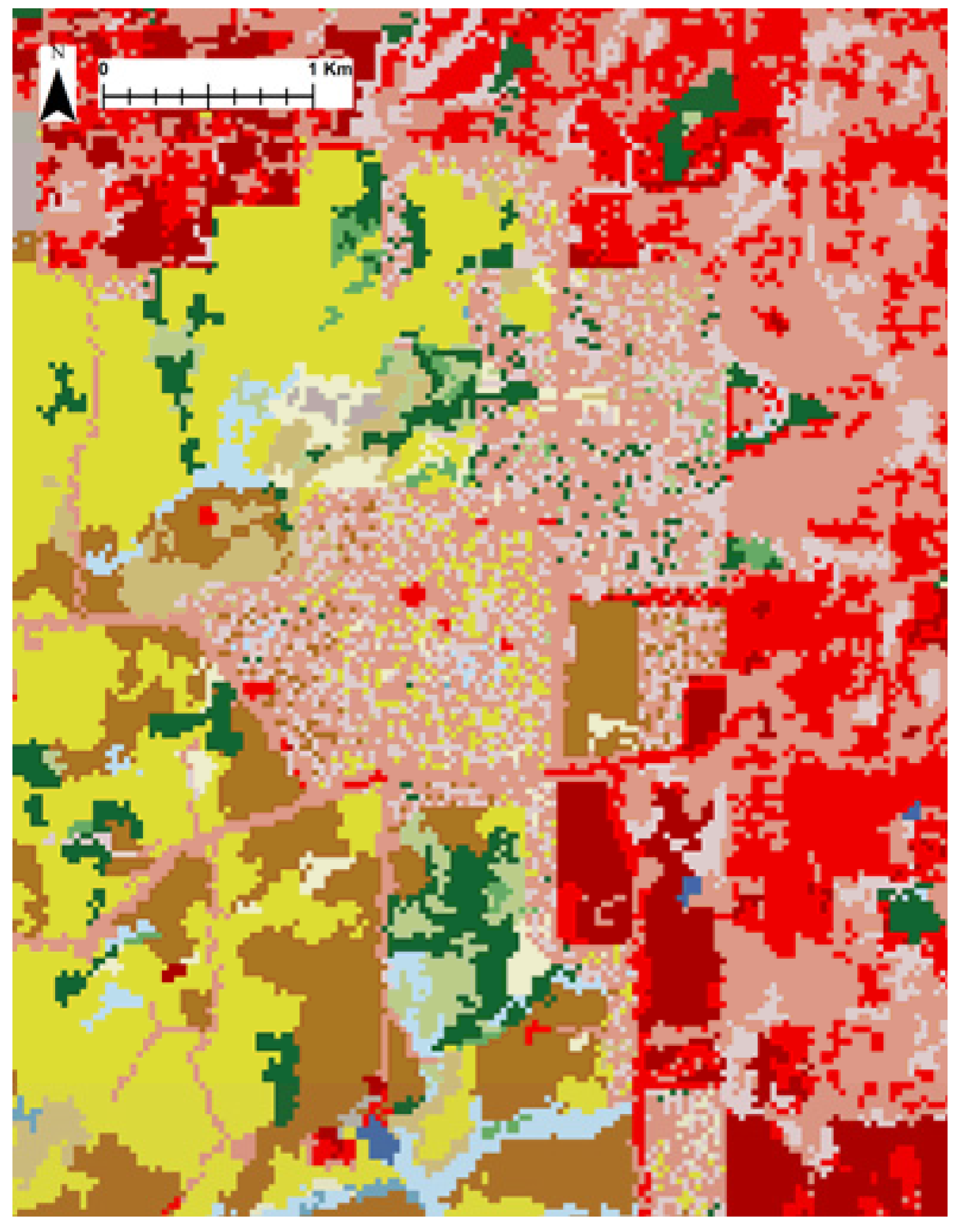
2.4. Mapping

| Urban Growth Boundary (UGB) | UGB Dist. | Zoning | Prime Farm Soils | Groundwater Restriction Zones | Measure 49 Claims | Geometric Mean | Weight | |
|---|---|---|---|---|---|---|---|---|
| Urban Growth Boundary (UGB) | 1 | 3 | 2 | 9 | 9 | 9 | 4.04 | 44% |
| UGB Distance | 1/3 | 1 | 1/2 | 7 | 9 | 5 | 1.94 | 21% |
| Zoning | 1/2 | 2 | 1 | 9 | 7 | 1 | 1.99 | 21% |
| Prime Farm Soils | 1/9 | 1/7 | 1/9 | 1 | 1/3 | 1/7 | 0.21 | 2% |
| Groundwater Restriction Zones | 1/9 | 1/9 | 1/7 | 3 | 1 | 5 | 0.55 | 6% |
| Measure 49 Claims | 1/9 | 1/5 | 1 | 7 | 1/5 | 1 | 0.56 | 6% |
| Total | 9.29 | 100% |
3. Results

4. Discussion
5. Conclusions
- (1)
- Although simple, our land cover projection requires the use of a quantitative GIS process to actually produce the maps, so it still faces the same issues of other scenario modeling efforts when translating qualitative data to quantitative.
- (2)
- Keeping the stakeholder consultation limited is advantageous, because it allows researchers to model future land cover under manageable time and effort constraints with widely available GIS data. Our land cover scenarios represent a gradient of potential realities based on the same storyline, and researchers still needed to make assumptions and set some of the parameters themselves.
- (3)
- The stakeholder consultation led to place specific analysis (e.g., different growth rates for urban vs. rural areas). The land use regulatory system is unique to Oregon, and the spatial data based on it encapsulates a great deal of external analysis that made our process faster. This highlights the potential difficulty in generalizing scenario development frameworks that facilitate reproducibility [15].
Acknowledgments
Author Contributions
Conflicts of Interest
References
- Millennium Ecosystem Assessment (MA). Ecosystems and Human Well-Being; Island Press: Washington, DC, USA, 2005. [Google Scholar]
- Foley, J.A.; DeFries, R.; Asner, G.P.; Barford, C.; Bonan, G.; Carpenter, S.R.; Chapin, F.S.; Coe, M.T.; Daily, G.C.; Gibbs, H.K.; et al. Global consequences of land use. Science 2005, 309, 570–574. [Google Scholar] [CrossRef]
- Seto, K.C.; Güneralp, B.; Hutyra, L. Global forecasts of urban expansion to 2030 and direct impacts on biodiversity and carbon pools. Proc. Natl. Acad. Sci. USA 2012, 109, 16083–16088. [Google Scholar] [CrossRef]
- Gulickx, M.M.C.; Verburg, P.H.; Stoorvogel, J.J.; Kok, K.; Veldkamp, A. Mapping landscape services: A case study in a multifunctional rural landscape in the Netherlands. Ecol. Indic. 2013, 24, 273–283. [Google Scholar] [CrossRef]
- Turner, B.L.; Lambin, E.F.; Reenberg, A. The emergence of land change science for global environmental change and sustainability. Proc. Natl. Acad. Sci. USA 2007, 104, 20666–20671. [Google Scholar] [CrossRef]
- Thompson, J.R.; Wiek, A.; Swanson, F.J.; Carpenter, S.R.; Hollingsworth, T.; Spies, T.A.; Foster, D.R. Scenario studies as a synthetic and integrative research activity for long-term ecological research. BioScience 2012, 62, 367–376. [Google Scholar] [CrossRef]
- Bateman, I.J.; Harwood, A.R.; Mace, G.M.; Watson, R.T.; Abson, D.J.; Andrews, B.; Binner, A.; Crowe, A.; Day, B.H.; Dugdale, S.; et al. Bringing ecosystem services into economic decision-making: Land use in the United Kingdom. Science 2013, 341, 45–50. [Google Scholar] [CrossRef]
- Goldstein, J.H.; Caldarone, G.; Duarte, T.K.; Ennaanay, D.; Hannahs, N.; Mendoza, G.; Polasky, S.; Wolny, S.; Daily, G.C. Integrating ecosystem-service tradeoffs into land-use decisions. Proc. Natl. Acad. Sci. USA 2012, 109, 7565–7570. [Google Scholar] [CrossRef]
- Boody, G.; Vondracek, B.; Andow, D.A.; Krinke, M.; Westra, J.; Zimmerman, J.; Welle, P. Multifunctional agriculture in the United States. BioScience 2005, 55, 27–38. [Google Scholar] [CrossRef]
- Santelmann, M.V.; White, D.; Freemark, K.; Nassauer, J.I.; Eilers, J.M.; Vaché, K.B.; Danielson, B.J.; Corry, R.C.; Clark, M.E.; Polasky, S.; et al. Assessing alternative futures for agriculture in Iowa, U.S.A. Landsc. Ecol. 2004, 19, 357–374. [Google Scholar] [CrossRef]
- Waldhardt, R.; Bach, M.; Borresch, R.; Breuer, L.; Diekötter, T.; Frede, H.; Gäth, S.; Ginzler, O.; Gottschalk, T.; Julich, S.; et al. Evaluating today’s landscape multifunctionality and providing an alternative future: A normative scenario approach. Ecol. Soc. 2010, 15, 30:1–30:20. [Google Scholar]
- Price, J.; Silbernagel, J.; Miller, N.; Swaty, R.; White, M.; Nixon, K. Eliciting expert knowledge to inform landscape modeling of conservation scenarios. Ecol. Model. 2012, 229, 76–87. [Google Scholar] [CrossRef]
- Westervelt, J.; BenDor, T.; Sexton, J. A technique for rapidly forecasting regional urban growth. Environ. Plan. B: Plan. Des. 2011, 38, 61–81. [Google Scholar] [CrossRef]
- Patel, M.; Kok, K.; Rothman, D.S. Participatory scenario construction in land use analysis: An insight in the experiences created by stakeholder involvement in the northern Mediterranean. Land Use Policy 2007, 24, 546–561. [Google Scholar] [CrossRef]
- Alcamo, J. The SAS approach: Combining qualitative and quantitative knowledge in environmental scenarios. In Environmental Futures: The Practice of Environmental Scenario Analysis; Alcamo, J., Ed.; Elsevier: Amsterdam, The Netherlands, 2008; pp. 123–150. [Google Scholar]
- Kok, K. The potential of fuzzy cognitive maps for semi-quantitative scenario development, with an example from Brazil. Glob. Env. Chang. 2009, 19, 122–133. [Google Scholar] [CrossRef]
- Walz, A.; Lardelli, C.; Behrendt, H.; Grêt-Regamey, A.; Lundström, C.; Kytzia, S.; Bebi, P. Participatory scenario analysis for integrated regional modelling. Landsc. Urban Plan. 2007, 81, 114–131. [Google Scholar] [CrossRef]
- Swetnam, R.D.; Fisher, B.; Mbilinyi, B.P.; Munishi, P.K.T.; Willcock, S.; Ricketts, T.; Mwakalila, S.; Balmford, A.; Burgess, N.D.; Marshall, A.R.; et al. Mapping socio-economic scenarios of land cover change: A GIS method to enable ecosystem service modelling. J. Environ. Manag. 2011, 92, 563–574. [Google Scholar] [CrossRef]
- Lamarque, P.; Artaux, A.; Barnaud, C.; Dobremez, L.; Nettier, B.; Lavorel, S. Taking into account farmers’ decision making to map fine-scale land management adaptation to climate and socio-economic scenarios. Landsc. Urban Plan. 2013, 119, 147–157. [Google Scholar] [CrossRef]
- Koschke, L.; Fürst, C.; Frank, S.; Makeschin, F. A multi-criteria approach for an integrated land-cover-based assessment of ecosystem services provision to support landscape planning. Ecol. Indic. 2012, 21, 45–56. [Google Scholar]
- Hulse, D.W.; Branscomb, A.; Payne, S.G. Envisioning alternatives: Using citizen guidance to map future land and water use. Ecol. Appl. 2004, 4, 325–341. [Google Scholar]
- Oregon Blue Book. City and County Populations. Available online: http://bluebook.state.or.us/local/populations/populations.htm (accessed on 21 August 2013).
- Oregon Metro. 20 and 50 Year Regional Employment and Population Range Forecasts. Available online: http://library.oregonmetro.gov/files/20–50_range_forecast.pdf (accessed on 4 April 2013).
- Portland State University College of Urban and Public Affairs Population Research Center. Population Estimates. Available online: http://www.pdx.edu/prc/population-estimates-0 (accessed on 19 August 2013).
- Fry, J.A.; Coan, M.J.; Homer, C.G.; Meyer, D.K.; Wickham, J.D. Completion of the National Land Cover Database (NLCD) 1992–2001 Land Cover Retrofit Product. Available online: http://pubs.usgs.gov/of/2008/1379/pdf/ofr2008-1379.pdf (accessed on 13 January 2014).
- Fry, J.; Xian, G.; Jin, S.; Dewitz, J.; Homer, C.; Yang, L.; Barnes, C.; Herold, N.; Wickham, J. Completion of the 2006 National Land Cover Database for the conterminous United States. Photgramm Eng. Remote Sens. 2011, 77, 858–864. [Google Scholar]
- Lambin, E.F.; Turner, B.L.; Geist, H.J.; Agbola, S.B.; Angelsen, A.; Bruse, J.W.; Coomes, O.T.; Dirzo, R.; Fischer, G.; Folke, C.; et al. The causes of land use and land cover change: Moving beyond myths. Glob. Environ. Chang. 2001, 11, 261–269. [Google Scholar] [CrossRef]
- Planning the Oregon Way: A Twenty-Year Evaluation; Abbot, C.; Howe, D.; Adler, S. (Eds.) Oregon State University Press: Corvallis, OR, USA, 1994.
- Oregon Department of Land Conservation and Development. Ballot Measures 37 (2004) and 49 (2007) Outcomes and Effects. Available online: http://www.oregon.gov/LCD/docs/publications/m49_2011-01-31.pdf (accessed on 1 April 2013).
- Oregon Department of Land Conservation and Development. Metro Urban and Rural Reserves. Available online: http://www.oregon.gov/LCD/Pages/metro_urban_and_rural_reserves.aspx (accessed on 1 April 2013).
- Boeder, M.; Chang, H. Multi-scale analysis of oxygen demand trends in an urbanizing Oregon watershed, USA. J. Environ. Manag. 2008, 87, 567–581. [Google Scholar] [CrossRef]
- Praskievicz, S.; Chang, H. Impacts of climate change and urban development on water resources in the Tualatin River basin, Oregon. Ann. Assoc. Am. Geogr. 2011, 101, 249–271. [Google Scholar] [CrossRef]
- Oregon Department of Environmental Quality. Tualatin Subbasin Total Maximum Daily Load and Water Quality Management Plan: Chapter 1—Overview and Background. Available online: http://www.deq.state.or.us/wq/tmdls/docs/willamettebasin/tualatin/revision/Ch0CoverExecSummary.pdf (accessed on 3 March 2013).
- Pratt, B.; Chang, H. Effects of land cover, topography, and built structure on seasonal water quality at multiple spatial scales. J Haz. Mater. 2012, 209/210, 48–58. [Google Scholar] [CrossRef]
- Chang, H.; Thiers, P.; Netusil, N.; Yeakley, J.A.; Rollwagon-Bollens, G.; Bollens, S.M. Relationship between environmental governance and water quality in a growing metropolitan area of the Pacific Northwest, USA. Hydro. Earth Syst. Sci. 2014, in press. [Google Scholar]
- Oregon Metro. RLIS Live, Geographic Information System Data. Available online: http://www.oregonmetro.gov/index.cfm/go/by.web/id=593 (accessed on 21 August 2013).
- City of Dayton, Oregon. Planning Atlas and Comprehensive Plan. Available online: http://www.ci.dayton.or.us/vertical/sites/%7B0813AE62-E15F-4C65-858B-10DDF2ABA1FE%7D/uploads/Complete_Copy_3-31-11.pdf (accessed on 11 March 2014).
- Oregon Spatial Data Library. Available online: http://spatialdata.oregonexplorer.info/geoportal/catalog/main/home.page (accessed on 21 August 2013).
- USFWS Geospatial Services. USFWS National Cadastral Data. Available online: http://www.fws.gov/GIS/data/CadastralDB/index.htm (accessed on 21 August 2013).
- Oregon Water Resources Department. Water Protections and Restrictions. Available online: http://www.oregon.gov/owrd/pages/pubs/aquabook_protections.aspx (accessed on 21 August 2013).
- Oregon State Archives. Department of Land Conservation and Development. Division 33; Agricultural Land. Available online: http://arcweb.sos.state.or.us/pages/rules/oars_600/oar_660/660_033.html (accessed on 27 September 2013).
- U.S. Census Bureau. Profile of General Population and Housing Characteristics: 2010. Geography: Portland-Vancouver-Hillsboro, OR-WA Metro Area (part); Oregon, USA, 2010. Available online: http://factfinder2.census.gov/faces/tableservices/jsf/pages/productview.xhtml?pid=DEC_10_DP_DPDP1&prodType=table (accessed on 19 August 2013). [Google Scholar]
- U.S. Bureau of Labor Statistics. Local Area Employment Statistics, U.S. Department of Labor. Available online: http://data.bls.gov/cgi-bin/dsrv (accessed on 19 August 2013).
- Oregon Metro. The Nature of 2040: The Region’s 50-Year Plan for Managing Growth. Available online: http://library.oregonmetro.gov/files/natureof2040.pdf (accessed on 28 January 2014).
- Environmental Science Research Institute. ArcGIS 10.1.; Environmental Science Research Institute: Redlands, CA, USA, 2010. [Google Scholar]
- Saaty, T.L. The Analytic Hierarchy Process: Planning, Priority Setting, Resource Allocation; McGraw-Hill: New York, NY, USA, 1980. [Google Scholar]
- Castella, J.; Trung, T.N.; Boissau, S. Participatory simulation of land-use changes in the northern mountains of Vietnam: The combined use of an agent-based model, a role-playing game, and a geographic information system. Ecol. Soc. 2005, 10, 27:1–27:32. [Google Scholar]
- Rounsevell, M.D.A.; Ewert, F.; Reginster, I.; Leemans, R.; Carter, T.R. Future scenarios of European agricultural land use II. Projecting changes in cropland and grassland. Agric. Ecosyst. Environ. 2005, 107, 117–135. [Google Scholar] [CrossRef]
- Parker, D.C.; Manson, S.M.; Janssen, M.A.; Hoffman, M.J.; Deadman, P. Multi-agent systems for the simulation of land-use and land-cover change: A review. Ann. Assoc. Am. Geogr. 2003, 93, 314–337. [Google Scholar] [CrossRef]
- Kok, K.; van Delden, H. Combining two approaches of integrated scenario development to combat desertification in the Guadalentín Watershed, Spain. Environ. Plan. B: Plan Des. 2009, 36, 49–66. [Google Scholar] [CrossRef]
- Southworth, J.; Marsik, M.; Qiu, Y.; Perz, S.; Cumming, G.; Stevens, F.; Rocha, K.; Duchelle, A.; Barnes, G. Roads as drivers of change: Trajectories across the tri-national frontier in MAP, the southwestern Amazon. Remote Sens. 2011, 3, 1047–1066. [Google Scholar] [CrossRef]
- Kelley, S.; (Washington County Land Use and Transportation Department, Hillsboro, OR, USA). Personal communication, 15 November 2012.
- Radeloff, V.C.; Nelson, E.; Plantinga, A.J.; Lewis, D.J.; Helmers, D.; Lawler, J.J.; Withey, J.C.; Beaudrey, R.; Martinuzzi, S.; Butsic, V.; et al. Economic-based projections of future land use in the coterminous Unites States under alternative policy scenarios. Ecol. Appl. 2012, 22, 1036–1049. [Google Scholar] [CrossRef]
- Suarez-Rubio, M.; Lookingbill, T.R.; Wainger, L.A. Modeling exurban development near Washington, DC, USA: Comparison of a pattern based model and spatially-explicit econometric model. Landsc. Ecol. 2012, 27, 1045–1061. [Google Scholar] [CrossRef]
- Yee, D.; (Oregon Metro, Portland, OR, USA). Personal communication, 11 July 2013.
- Walker, P.A.; Hurley, P.T. Planning Paradise: Politics and Visioning of Land Use in Oregon; The University of Arizona Press: Tucson, AZ, USA, 2011. [Google Scholar]
- Peterson, G.D.; Cumming, G.S.; Carpenter, S.R. Scenario planning: A tool for conservation planning in an uncertain world. Conserv. Biol. 2003, 179, 358–366. [Google Scholar]
© 2014 by the authors; licensee MDPI, Basel, Switzerland. This article is an open access article distributed under the terms and conditions of the Creative Commons Attribution license (http://creativecommons.org/licenses/by/3.0/).
Share and Cite
Hoyer, R.W.; Chang, H. Development of Future Land Cover Change Scenarios in the Metropolitan Fringe, Oregon, U.S., with Stakeholder Involvement. Land 2014, 3, 322-341. https://doi.org/10.3390/land3010322
Hoyer RW, Chang H. Development of Future Land Cover Change Scenarios in the Metropolitan Fringe, Oregon, U.S., with Stakeholder Involvement. Land. 2014; 3(1):322-341. https://doi.org/10.3390/land3010322
Chicago/Turabian StyleHoyer, Robert W., and Heejun Chang. 2014. "Development of Future Land Cover Change Scenarios in the Metropolitan Fringe, Oregon, U.S., with Stakeholder Involvement" Land 3, no. 1: 322-341. https://doi.org/10.3390/land3010322
APA StyleHoyer, R. W., & Chang, H. (2014). Development of Future Land Cover Change Scenarios in the Metropolitan Fringe, Oregon, U.S., with Stakeholder Involvement. Land, 3(1), 322-341. https://doi.org/10.3390/land3010322