Uncovering Dominant Land-Cover Patterns of Quebec: Representative Landscapes, Spatial Clusters, and Fences

Abstract

Mapping large areas for planning and conservation is a challenge undergoing rapid transformation. For centuries, the creation of broad-extent maps was the near-exclusive domain of expert specialist cartographers, who painstakingly delineated regions of relative homogeneity with respect to a given set of criteria. In the satellite era, it has become possible to rapidly create and update categorizations of Earth’s surface with improved speed and flexibility. Land cover datasets and landscape metrics offer a vast set of information for viewing and quantifying land cover across large areas. Comprehending the patterns revealed by hundreds of possibly relevant landscape metric values, however, remains a daunting task. We studied the information content of a large set of landscape pattern metrics across Quebec, Canada, asking whether they were capable of making consistent, spatially cohesive distinctions among patterns in landscapes. We evaluated the possibility of metrics to identify representative landscapes for efficient sampling or conservation, and determined areas where differences in nearby landscape patterns were the most and least pronounced. This approach can serve as a template for a landscape perspective on the challenges that will be faced in the near future by planners and conservationists working across large areas.

1. Introduction

It is a longstanding challenge to appropriately map large areas for conservation and planning. Scientists typically use a variety of mapping approaches that classify broad regions according to a range of criteria: these include terrestrial eco-region maps [1], environmental domain classifications [2,3], and continental-scale biogeographical regionalizations [4,5]. Many scientists rely on these products for research questions, while resource managers need them for better planning of resource uses [6].

The enormous spatial scale of climate change will demand a sophisticated and complex understanding of the many ways that large areas may contain both large-scale patterns and fine-scale granularity. As systematic planning efforts to cope with climate change begin at local [7], regional [8,9], and continental [10] scales, we can expect a pressing need to understand regions via strategies that can consider multiple criteria, produce flexible outputs, and ingest large amounts of new information.

As planners contemplate specific ways to manage resources in a context of climate change [11], it is important to recognize that typical broad-scale classification maps are limited in several ways that can have important implications in their use for large-scale planning. First, regionalization of environmental factors into closed, contiguous polygons inherently implies a generalization of many phenomena [6]. Second, because most polygon-based maps do not quantify or locate variability within regions [5], it is difficult to know which areas within a polygon best represent its nominal characteristics. Third, local variations in environmental drivers may cause the patterns to change across space and time [12,13]. In Quebec, Canada, for example, landscape patterns at any moment are a function of many abiotic, biotic, and human factors operating simultaneously at multiple temporal and spatial scales [14,15,16,17,18].

In addition to polygon-based ecological classification maps, scientists have access to an increasing number of high quality raster-based data sets that quantify phenomena across large areas. Satellite-based land-cover maps, in particular, present a characterisation of the ground surface composition at a much finer scale than that of most polygon-based maps [19,20,21]. Building on the production of land-cover maps, analysis techniques are in rapid expansion for biophysical regionalizations [2,4], ecoregion delineation [5,22], object-based classification [23,24,25], and data sets fusing data from both raster and polygon sources [26,27,28,29,30,31].

To better understand and use land-cover patterns, a large set of landscape metrics has been developed in landscape ecology to quantify both the composition and configuration of landscape patterns [32]. Typically, they are used in studies seeking to understand relationships between spatial characteristics of landscapes and ecological processes [13]. Though mostly used in small areas with mixed success [33,34], landscape metrics calculated across large areas have been integrated as data for large-scale ecological investigations, notably for national or global assessments [35,36,37,38]. Nearly all of these maps have focused on measures that are rooted in, or exclusively linked to, the proportion of a phenomenon in a given area. Studies typically target a small set of individual metrics mapped across large areas, often to characterize forest fragmentation [36,37,39,40,41]. Thus far, limited consideration has been paid to the question of the information content among a large set of metrics across large areas, in part because of the challenges of interpreting and computing such large datasets over vast spatial extents [42].

To improve comprehension of the information contained in large geographic data sets, researchers can group landscapes, using a variety of quantitative clustering methods [5,43]. This allows the variability in the data to be compressed, and because of the geographic context, cluster membership can be spatially visualized through maps [42,44]. An increasing number of studies have proposed to highlight the best representatives of each group for further consideration, by identifying “exemplars” [45,46,47], “centroids” [5,44], or “medoids” [42,48]. Complementary to relatively dense numerical tables of characteristics to summarize landscape characteristics, representative landscapes have the ability to summarize an immense area into a small set of objectively identified specific places that can be used for careful planning or monitoring of resources [19,46,49].

In Quebec, a large province of Canada spanning nearly 20 degrees of latitude and 23 degrees of longitude, there are existing maps of forest characteristics and bioclimatic zones [3], but no comprehensive interpretation of the observable land-cover patterns across the province. To better understand the baseline patterns of forest composition and configuration across this vast area, we pursued three objectives. First, we explored the information content of an extensive set of landscape pattern metrics covering the forested land cover of the province, to investigate whether landscape metrics were suitable for partitioning landscapes of a large area into distinct, consistent and spatially cohesive regions. Second, we assessed the capability of metrics to distinguish representative landscapes that could be used as sampling units or sites for long-term study or conservation. Third, we determined where differences in landscape patterns were the most and least pronounced between adjacent landscapes over the whole province. The approach in this article demonstrates an effective set of strategies to synthesize both the composition and configuration of Quebec’s forested land, and will serve as a template for a landscape perspective for challenges that will be faced in the near future by planners and conservationists working across large areas.

2. Material and Methods

2.1. Study Area

This research focused on the forested landscapes of Quebec, Canada (Figure 1). The province of Quebec is a vast 1.3 million km² region [50] located between 45°N–63°N and 57°W–79°30'W (Figure 1). Landscape patterns are perpetually modified by the interplay of a wide array of natural drivers and regimes [40,51], many different disturbance sources such as fires, insect outbreaks and logging [15,16,17,18,52]; patterns are composed of diverse vegetation cover types appearing throughout the Province. At this scale, the main drivers of landscape covers are the substantial climatic gradient occurring from south to north (across 1,900 km), and, to a lesser extent, soil type, topography and variation in precipitation regimes [3]. These drivers divide the province into broad regions [3] and the Ministère des Ressources naturelles du Québec (MRN) delineated five vegetation subzones (Figure 1) according to dominating vegetation at climax [51]: (A) the hardwood forest, comprised prominently of sugar maple, yellow birch, basswood, and bitternut hickory; (B) the mixed forest, comprised of species such as balsam fir and yellow birch; (C) the continuous boreal forest, comprised of black spruce, mosses, lichen, balsam fir, and white birch; (D) the taiga, comprised of black spruce, lichens; and (E) the forested tundra, of dwarf black spruce and lichens. Disturbances substantially affect the patterns in some subzones. In the boreal forest (Figure 1, site C), patterns are influenced by fire regimes and by forestry activities [15]. The mixed forest (Figure 1, site B), closer to population centers, is also affected by forest industries and fires [16]. The hardwood forests (Figure 1, site A) have been modified by the human activities of farming, urban settlements and forestry for hundreds of years [17,52].

Figure 1. Earth Observation for Sustainable Development of Forests land-cover (EOSD) land cover in the province of Quebec, Canada. Ministère des Ressources naturelles du Québec (MRN) vegetation subzones (black lettering) express the broad spatial variability along the large bioclimatic gradient. Subzones are (A) hardwood forest; (B) mixed forest; (C) continuous boreal forest; (D) taiga; (E) forested tundra. Subzone F in far northern Quebec is non-forested and not part of the EOSD forest classification. Some smaller land-cover categories were combined to increase interpretability.

Figure 1. Earth Observation for Sustainable Development of Forests land-cover (EOSD) land cover in the province of Quebec, Canada. Ministère des Ressources naturelles du Québec (MRN) vegetation subzones (black lettering) express the broad spatial variability along the large bioclimatic gradient. Subzones are (A) hardwood forest; (B) mixed forest; (C) continuous boreal forest; (D) taiga; (E) forested tundra. Subzone F in far northern Quebec is non-forested and not part of the EOSD forest classification. Some smaller land-cover categories were combined to increase interpretability.

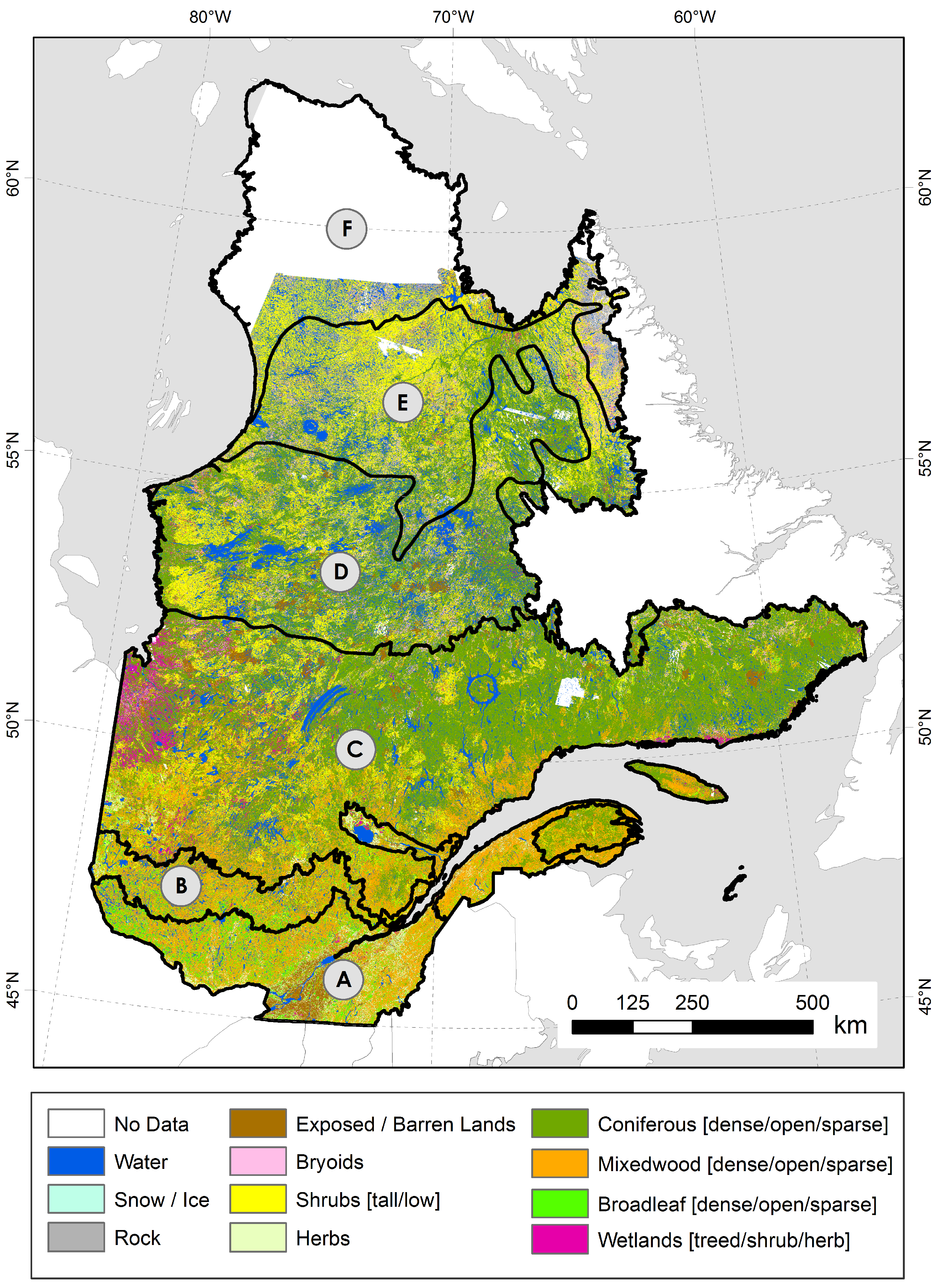
2.2. Land-Cover Data and Landscape Metrics

To characterize the land-cover composition of landscapes in Quebec, we used the Earth Observation for Sustainable Development of Forests land-cover (EOSD) data set [50,53]. The EOSD data set is a freely available product derived from Landsat-7 imagery resampled at 25-meter pixels with the nominal data collection of year 2000. The EOSD project categorizes Canada’s forested regions with 23 different land-cover classes [49] (background in Figure 1). The EOSD product did not categorize northern non-forested regions above the forested tree line (the blank zone F in Figure 1); they were excluded from this study.

We used the EOSD mosaic of Quebec to generate landscapes for which we calculated landscape metrics for consideration. Using the framework of the Canadian National Topographic System 1:50,000 scale sheet borders, we cut the study area into 1,398 rectangular shaped raster landscapes of about 900 km² having 25-meter pixels. The 23 possible classes were reduced to 20 usable classes, by combining the unusable categories “shadow”, “cloud”, and “unclassified”, with the existing “no data” class. This particular cutting frame was performed to be consistent with existing large-scale studies [36,47,49]. To ensure future potential for comparison across jurisdictional lines, the metric set was the same large set of calculations used in Cardille and Lambois [46]. For each landscape, Fragstats v3.3 [54,55] was used to calculate 90 pattern metrics at the landscape level and 90 at the class level (for each of the possible 20 classes found in a landscape), resulting in a set of 1,890 landscape metric values for each of the 1,398 landscapes.

2.3. Extracting Information from Metric Values: Clustering and Determining Representatives

Because landscape pattern metric values are numbers with different orders of magnitude, and may well be correlated [34,54], we followed the protocol of Cardille and Lambois [46] and performed a principal component analysis on the metric set to form a set of orthogonal meta-metrics [56,57,58]. This revealed the depth of the redundancy in the full landscape metric set: a vector of 85 measures was sufficient to capture 90% of the variation in the large set. Despite the low information value of individual principal components beyond the 85th, we retained the full set of 1,398 principal components to assess landscapes based on all the information that might distinguish landscapes from each other. This use of the full information content was not significantly more computationally demanding and avoided an arbitrary cutoff.

To estimate the differences between the landscape patterns of each pair of landscapes, we calculated the Euclidean distance between their values along the principal components axes. For a pair of landscapes a and b, the difference between their land-cover patterns was computed as:

d_a,b = sqrt((PC1_a − PC1_b)² + … + (PC1398_a − PC1398_b)²)

(1)

The matrix of differences between all pairs of landscapes was used as input to the affinity propagation algorithm to perform a clustering analysis [45]. That algorithm clusters more efficiently than the better-known k-means algorithm, while it simultaneously identifies an item from the set that best represents each cluster [45]. Using the apcluster package [59] in R [60], we clustered the landscape set in 55 clustering iterations, each with a specified number of clusters (k = 2 to 50, 55, 60, 65, 70, 75, and 100) and the corresponding number of exemplars. To understand the distribution of landscape pattern in space and assess the spatial pattern of differences within a cluster of landscapes, we developed a “centrality” map of the similarity in landscape pattern of every cluster to its exemplar [44].

2.4. Spatial Fences

We computed “spatial fences” [44] to identify the most significant borders among all the different landscape pattern types in Quebec. Spatial fences represent cluster boundaries that appeared repeatedly across the iterations of different numbers of clusters; boundaries that appeared repeatedly over the same area, especially for the coarsest regionalizations of landscapes, identified the most important variation of patterns among adjacent landscapes in forested Quebec. Fences do not form the closed polygons seen in most traditional ecological regionalization work [44]; rather, they occur at the edges of where landscapes were similar enough to be consistently grouped together across several sets of clusters. To illustrate the degree of importance of each fence, fences were mapped with varying thickness [44]. Thicker segments represented more noteworthy fences, and the thickness was set using two criteria. First, we added an inversely proportional weight on the number of clusters; we made borders between spatial clusters thicker if the “k” was small. As a result, the borders of the clustering with two groups were the strongest and thus drawn more thickly than others. Second, thickness was also determined by the existence of a division between cluster types in more than one clustering iteration. Hence, the thickest fences present the location of the most fundamental and pronounced changes in landscape patterns in the province.

3. Results

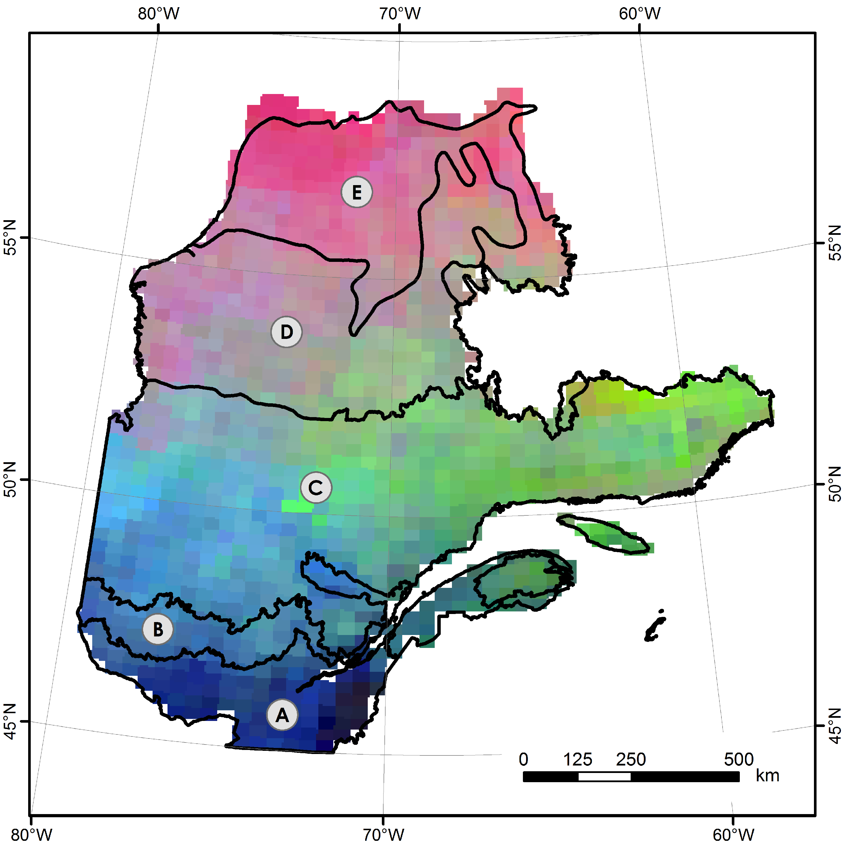
3.1. Composite Image of PCA Values

The main characteristics of landscape patterns change gradually across Quebec (Figure 2). Across the wide spectrum of bioclimatic conditions and the multitude of drivers generating land cover patterns in the province, areas with similar conditions are grouped together in space. For example, northern patterns were characterized by extreme values on the first principal component, while landscapes located in the south-central part of Quebec represented different combinations of the three principal components.

Imaging the first three principal components (Figure 2) reveals some of the ways regionalized patterns of land cover are spatially arranged across Quebec. The forested tundra subzone (Figure 2, site E) contains relatively homogeneous land-cover patterns that differ strongly from those of southern Quebec, as noted by extreme values along the first principal component from landscapes in the rest of the province. The hardwood forest subzone (Figure 2, site A) is also characterized by relatively homogeneous land-cover patterns. The mixed forest, the continuous boreal forest and the taiga subzones also reveal mostly distinct patterns, as variations in the three first principal components among these zones are visible (Figure 2). Additionally, they are presenting a clear latitudinal structure. The visible difference between the patterns in the eastern and western part of the continuous boreal forest (Figure 2, site C) is consistent with the land-cover data (Figure 1), where a clear distinction in landscape composition divides the boreal forest from the taiga. It is also consistent with major differences in hydrologic regimes characterizing the eastern from the western part of boreal forest [3].

Figure 2. Composite image comprised of the three first principal components of landscape metric values (PC1 in red, PC2 in green, PC3 in blue). Each square cell represents an individual landscape.

Figure 2. Composite image comprised of the three first principal components of landscape metric values (PC1 in red, PC2 in green, PC3 in blue). Each square cell represents an individual landscape.

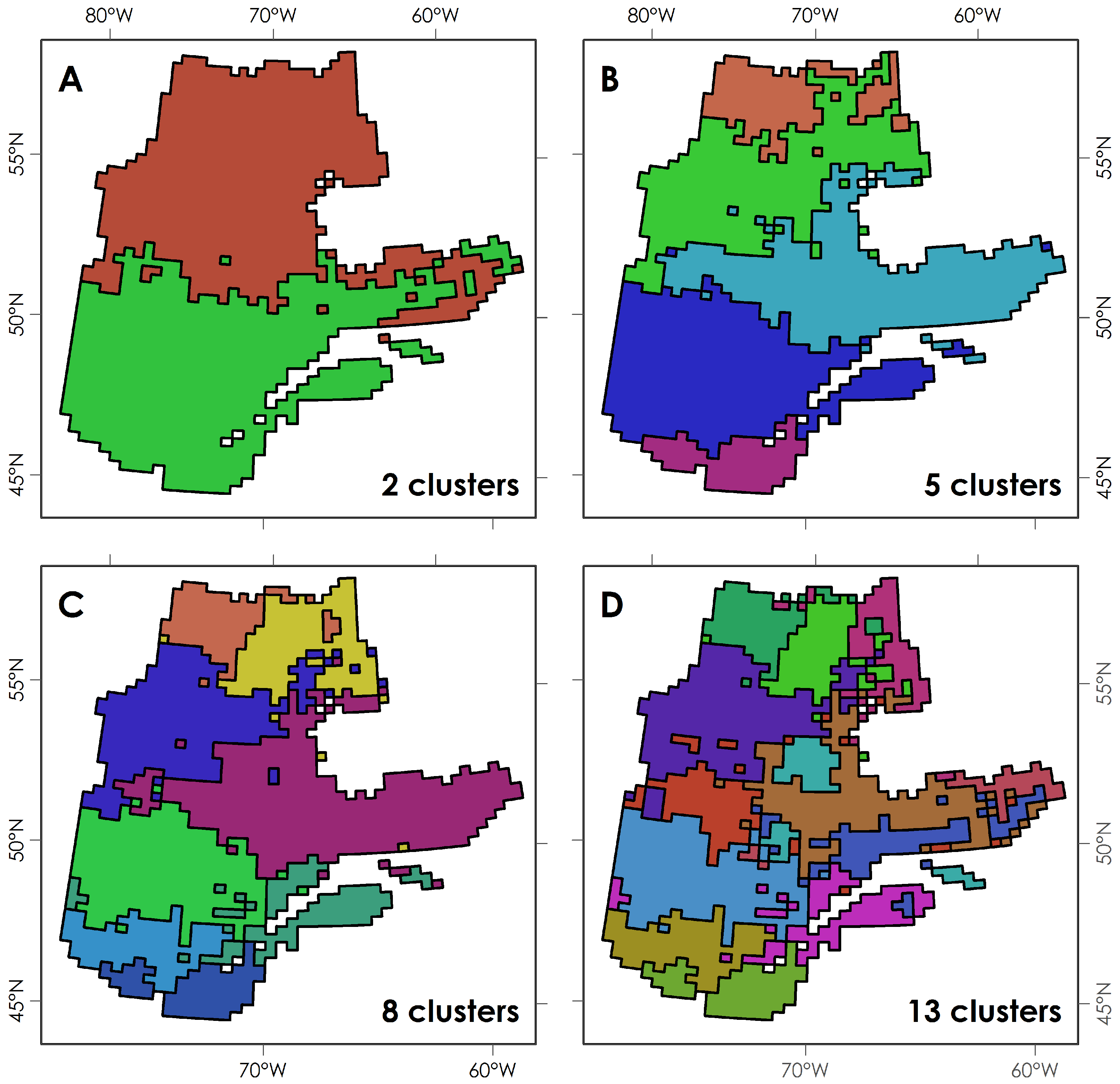
3.2. Spatial Clusters

Despite the fact that no positional information (i.e., coordinates, zones, etc.) was included in the similarity and clustering processes, classifications of landscapes of Quebec display a strong and consistent spatial cohesion across a wide range of cluster counts (Figure 3). Across a range of cluster numbers (Figure 3), landscapes grouped together by landscape metrics were largely homogeneously grouped when mapped in geographic space. Clustering of landscapes into five groups, for example as shown in Figure 3B, revealed cohesive patterns in metric space, as well as being homogeneously grouped in space. Clustering similar landscapes using only landscape metrics did not generate arbitrarily arranged clusters in geographic space. Rather, clusters of landscape pattern types are highly spatially organized and this structure largely corresponds to the provincial latitudinal gradient. The spatial cohesion of clusters of landscape metric values is so pronounced that they can be considered as a potential partitioning of land-cover characteristics of Quebec. With few exceptions, clusters were almost entirely spatially contiguous (Figure 3).

Figure 3. Unconstrained clustering using landscape pattern metrics showing partitioning of Quebec into 2 (A), 5 (B), 8 (C), and 13 (D) groups.

Figure 3. Unconstrained clustering using landscape pattern metrics showing partitioning of Quebec into 2 (A), 5 (B), 8 (C), and 13 (D) groups.

The classified pattern (Figure 3) values are roughly consistent with Quebec’s major bioclimatic drivers (Figure 1). First, clustering outputs illustrate a latitudinal structure in spatial distribution of land-cover patterns based on the bioclimatic gradient. When looking at maps of Figure 3A–C, the north-south structure is clear. For runs with higher numbers of clusters (Figure 3C,D), clusters tend to partition the geographic space from west to east along 70°W. That is also consistent with more local- or regional-scale factors such as hydrological regimes and other edaphic factors having consequences on vegetation growth and, presumably, landscape patterns [3,61].

With little exception, landscapes that were near each other in metric space were also near each other in geographic space. Landscapes that were the most similar to their exemplar also strongly tended to be those that were among those geographically nearest to it (Figure 4, right panel); geographically distant landscapes were generally less similar (lighter colours near cluster boundaries). This representation of the exemplars’ geographic and numeric centrality reveals the intra-group homogeneity as well as the inter-group heterogeneity. For example, within-group homogeneity can be seen in cluster #3 where similarity values are mostly uniform across the cluster. On the other hand, inter-group heterogeneity can be observed in at least two ways on geographic space. One example is a gradual transition of patterns exemplified by a distinctive strip of light coloured cells on common frontiers between clusters #1 and #2. A much different example is found at the border of clusters #4 and #5 where sharper distinction among patterns is seen.

Figure 4. Clustering set of five with representative landscapes located within their clusters in Quebec. In the centrality map, measures of centrality are represented with colour ramps (darker colours represent higher similarity of landscapes to their exemplar, lighter colours represent lower similarity values.

Figure 4. Clustering set of five with representative landscapes located within their clusters in Quebec. In the centrality map, measures of centrality are represented with colour ramps (darker colours represent higher similarity of landscapes to their exemplar, lighter colours represent lower similarity values.

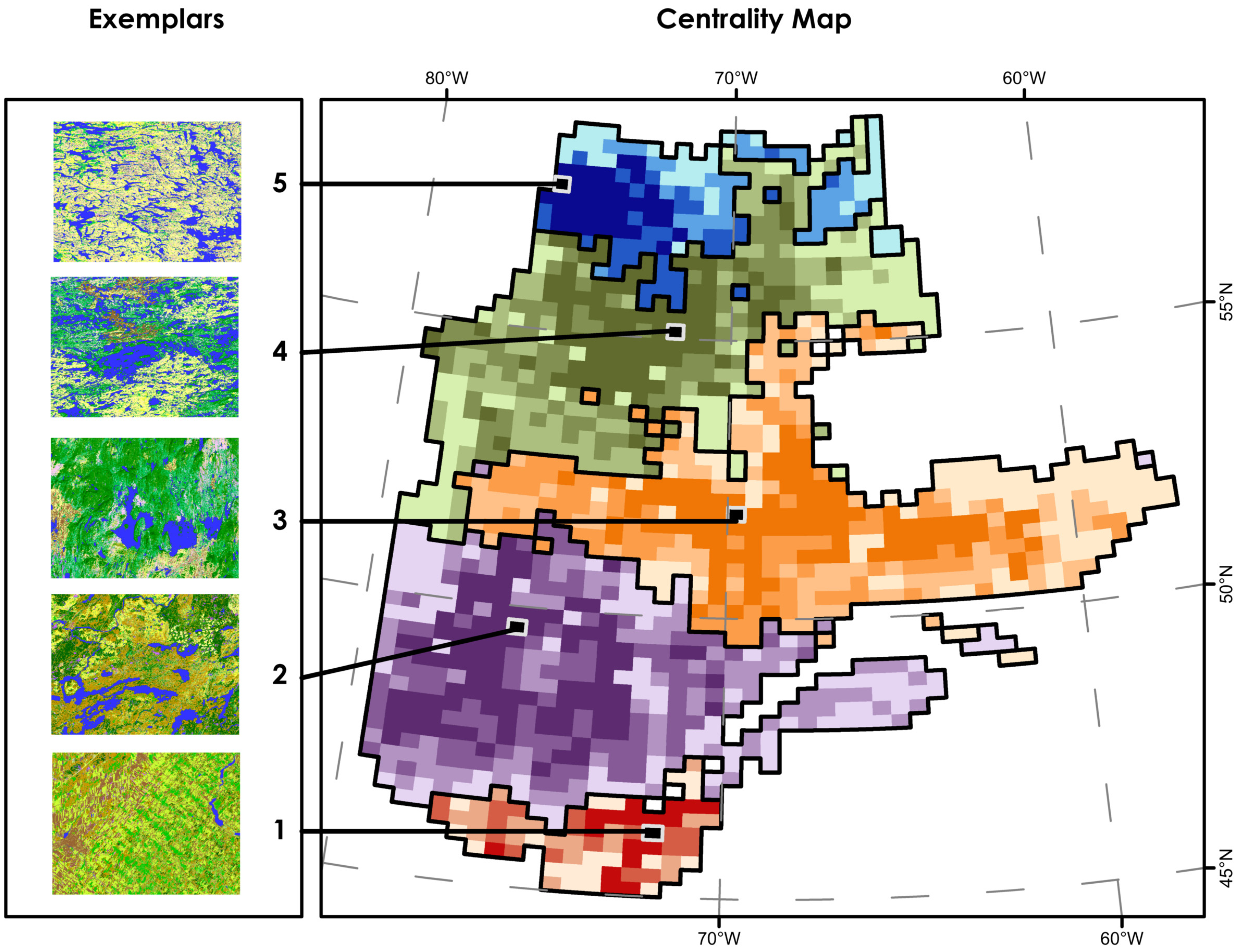
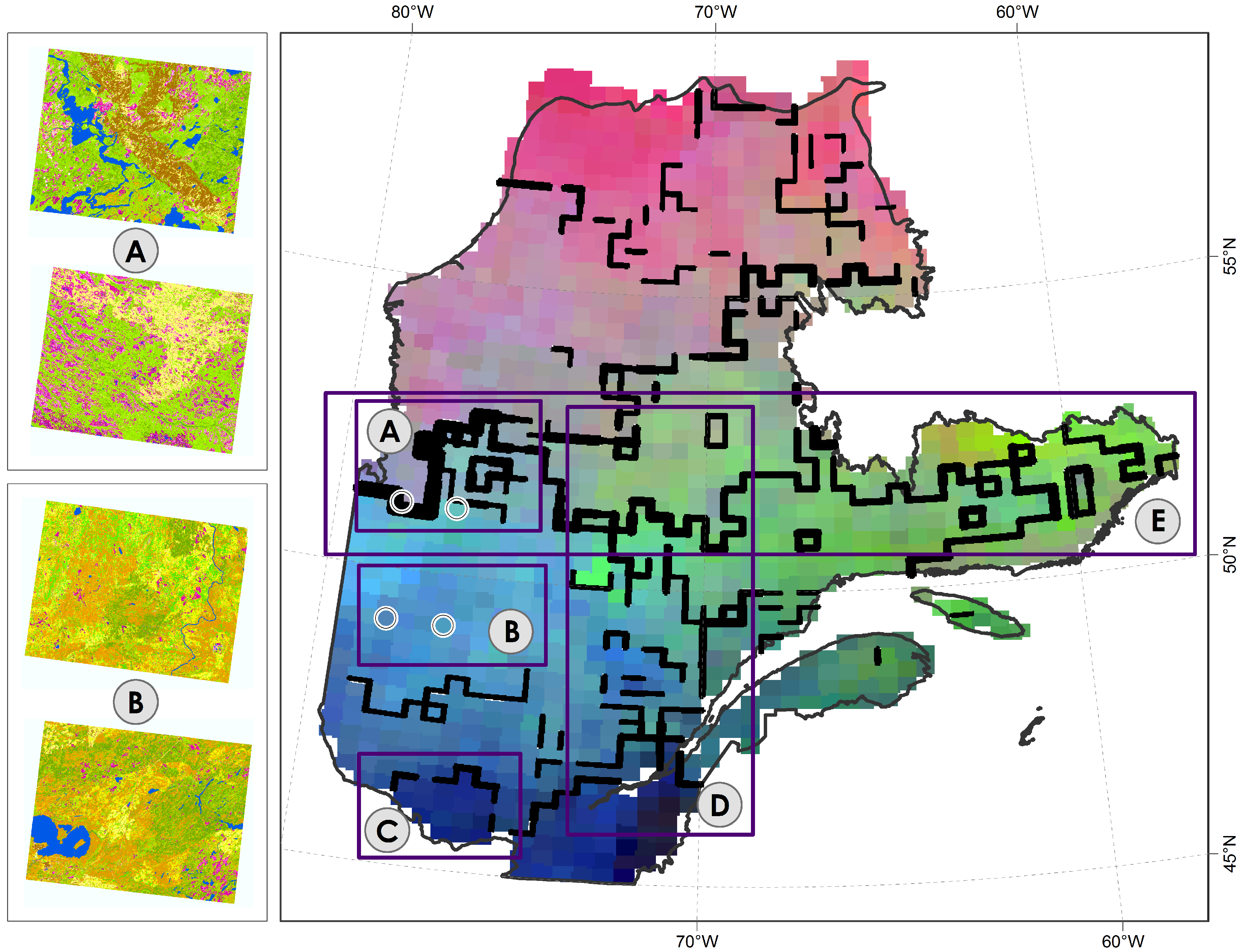
3.3. Representative Land-Cover Patterns of Forested Quebec

Exemplars given by the affinity propagation algorithm visually summarize landscape patterns found within clusters (Figure 4, left panel). The spatial distribution of representative landscapes (Figure 4) follows a latitudinal spatial distribution similar to the vegetation composition based on the bioclimatic divisions evident in Figure 1 [51]:

• “Exemplar 1—pasture lands and broad-leaf forest” (Figure 4, #1) is a landscape dominated by a mixed of pasture-lands (herbs) and croplands (exposed lands), and patches of dense broad-leaf forest. This landscape corresponds to the typical southern Quebec agricultural landscape with its human induced patterns—square shaped patches—rather than natural land cover patterns, which is consistent with Pan et al. [52].
• “Exemplar 2—mixed forest” (Figure 4, #2) is composed of dense mixed-wood and dense coniferous forest, and logging patterns are also very noticeable with networks of square-shaped “shrub” patches linked by thin straight forest roads, human induced patterns such as those from logging, and highly linear patches (roads, power transmission line corridors, rail roads). These patterns match expectations based on previous studies [16,17].
• “Exemplar 3—Eastern Boreal forest” (Figure 4, #3) is characterized by dense and continuous coniferous forest with some sparse patches of bryoids, shrubs, and exposed lands. This landscape presents a composition similar to the description of the continuous boreal forest [51].
• “Exemplar 4—taiga and northern transition forest” (Figure 4, #4) is comprised of very large patches of sparse-open coniferous forest and shrubs, and widespread water bodies. This is consistent with the taiga description of open coniferous forests paired with lichen soil cover [51].
• “Exemplar #5—shrubby tundra” (Figure 4, #5) is mainly represented by shrubs and lakes, and composed of sparse coniferous patches along water patches sides, typical of northern Quebec and similar to the forested tundra description [51].

3.4. Spatial Fences

Superposing the divisions between repeated clustering iterations illustrates regions of Quebec according to land-cover patterns, and the resulting spatial fences identify the most pronounced variation in land-cover patterns among adjacent landscapes across forested Quebec (Figure 5). The degree of importance in pattern differences is represented by the thickness of fences between landscapes: thickest fences identify the most important landscape pattern differences at the provincial scale (Figure 5, box A), while thinner fences represent differences that are less important, but still noteworthy at this scale (Figure 5, box C). Pattern-derived regions defined with spatial fences are not neatly closed polygons (as in Figure 4); areas with no fence segments are those where pattern differences across space are too gradual to form break points between cluster types (box B). On close inspection, landscapes on opposite sides of a thick fence (Figure 5, box A, left panel) often have landscape composition and configuration that are much more different than landscape pairs with no thick fence between them (Figure 5, box B, left panel). The thinnest fences shown were borders between clusters that occurred at least 5 times (e.g., Figure 5, box C) across the clustering levels. The thickest fences, on the other hand, reappeared more than 16 times (Figure 5, box A), and they clearly correspond to large differences in the first three principal components of land-cover metrics (Figure 2).

Spatial fences delineate relatively sharp pattern changes in geographic space, and expose at least two interesting facts about Quebec landscape patterns. A first thing to note is the major fence that occurs along the 52°N line (Figure 5, box E), this fence is among the most pronounced in the study area and it divides the province into two regions between South, where patterns are mainly dominated with higher forest densities, and North, where patterns are mostly characterized by sparsely forested patches [51]. This important fence roughly matches the current northern commercial logging limit, which was delimited in part by biophysical and stand productivity constraints [62]. Second, spatial fences identify at least two kinds of regions of landscape patterns of Quebec; there are relatively “pure” regions and “mixed” regions. Pure regions (Figure 5, box B) are areas where landscape are characterized by strongly homogeneous patterns compared with nearby landscapes, where no fences were found more than 5 times during the clustering iterations. Mixed regions, in contrast, are those where considerable differences exist among landscapes in a relatively concentrated area (e.g., Figure 5, box D).

Figure 5. Spatial fences in forested Quebec. Borders between clusters across iterations reveal the most and least pronounced variation among adjacent landscapes in forested Quebec. Thickness of fences represents the degree of magnitude in pattern dissimilarities: thicker fences locate more important changes, and gaps locate gradual changes in landscape patterns.

Figure 5. Spatial fences in forested Quebec. Borders between clusters across iterations reveal the most and least pronounced variation among adjacent landscapes in forested Quebec. Thickness of fences represents the degree of magnitude in pattern dissimilarities: thicker fences locate more important changes, and gaps locate gradual changes in landscape patterns.

4. Discussion

4.1. Landscape Pattern Information and Clustering

The total information content of the set of landscape metrics for forested Quebec revealed that landscape patterns in Quebec are markedly structured cohesively in space, and that clusters of patterns are broadly consistent with what can be seen in the EOSD data. Although multiple principal component axes were used for precision when quantifying differences among landscapes, the image of the three first principal components contained considerable information on pattern spatial distribution across our large study area. This image map also helped us to envision how the clustering algorithm would partition landscapes throughout Quebec.

Clustering results suggest that landscape metrics are powerful enough to reveal the general structure in landscape pattern geographic distribution over Quebec. Clusters of landscape metric values were highly spatially aggregated and, surprisingly to us, quite cohesively homogeneous throughout the province. They revealed that landscape patterns in the province of Quebec vary, for lower numbers of cluster scenarios, principally along a south-north axis and, for greater numbers of cluster scenarios, in more complex ways longitudinally. This spatial structure, which relates with broad-scale patterns of bioclimatic drivers, brought new insights on how we can understand Quebec forested landscapes.

Given the consistent spatial coherence across a large number of cluster solutions, these results suggest that this approach to partitioning does indeed reveal highly useful landscape information. Landscape pattern metrics help to understand and group landscape conditions in Quebec, unlike other classifications that are largely based on expected late-successional state of vegetation conditions. Consequently, clustering results represent a new type of biogeographical information that could contribute to future broad-scale ecological planning and conservation efforts. The quantitative and flexible approach presented here might be adapted for tracing new ecological regions by combining various types of relevant ecological ancillary data for specific needs.

In contrast to the regionalization of British Columbia of Long et al. [42], our metric-based clusters formed groupings that were spatially contiguous. This may be due to several factors. First, because Long et al. used substantially fewer metrics (6 vs. more than 1,000 in this study), they may have had less total information available with which to successfully discriminate among landscapes. Additionally, because their study was on a much smaller area (5.5 × 10⁴ km² vs. 1.3 × 10⁶ km² here) using much smaller study units (1 km² vs. 900 km² here), their processing might have searched for much finer-scale variation than in our provincial-scale coarse partitioning to cluster major landscape types. Third, their study region (mountainous British Columbia) may simply contain much more spatial variation than Quebec notably through its extreme terrain variation, which can cause noteworthy changes in land cover patterns at fine scale. The intriguing differences and similarities suggest a need for deeper research on the use of landscape pattern metrics to delineate regions over large areas.

The results of this spatial clustering analysis are promising, and not limited in any way to the identification and mapping of land-cover patterns. Most immediately, the relation of landscape structure and biodiversity suggests that there may be potential to use this result to estimate biodiversity distribution or identify hotspots of biodiversity. More broadly, additional environmental descriptors could be incorporated in this approach to fit different classification needs. Biophysical data (soils nutrient concentrations, precipitations, sunlight exposure, etc.) could be used to create a more complete ecological-oriented map, and/or to separate differing landscapes within an existing ecological zone. This model could be used outside forests as well—for example for the clustering of lakes using chemical data or satellite signatures. Lakes could be separated into a desired number of groups with target lakes identified as exemplars, leading to a considerably more efficient field campaign.

4.2. Representative Landscapes

Representative landscapes, available through the clustering algorithm used here, provide an efficient way of objectively summarizing the information content of a large and complex landscape pattern metric data set [43,44]. Here, exemplars followed, with few exceptions, the general expectations based on the broad-scale bioclimatic gradient. The two southernmost exemplars (#1—pasture lands and broad-leaf forest and #2—mixed forest) revealed clear patterns of the human land uses of farming and logging. In this setting, where a set of real-world landscapes can be viewed or visited, small sets of exemplars are likely easier to interpret and to quickly understand than only summary tables of metric values [46,47]. In our opinion, this could be a very useful way of generalizing complex scientific research results on landscape patterns, thus aiding managers, policymakers and conservationists.

Representative landscapes may be useful in a variety of applications for studying forested landscapes in Quebec or any other large area. Geographers, landscape ecologists, resource managers, and conservationists could reasonably use exemplars as representative sampling landscapes for broad scale ecological studies or for comparing different conservation approaches on representative landscape patterns. For example, these exemplars could help managers identify a representative province-scale network of study sites [63], or to verify the spatial representativeness of existing study sites [44] or parks and protected areas [47] in relation to an entire study area.

4.3. Spatial Aspect of Land-Cover Patterns

With a geographic representation of each landscape’s similarity to its representative, it is possible to easily assess within-group homogeneity and locate between-group borders [43]. From this information, field ecologists could then use such information to efficiently sample from representative landscapes while avoiding non-characteristic conditions in their field campaigns. Additionally, the homogeneity of clusters could be useful to locate landscape pattern transition zones over Quebec, for example, where boundaries between clusters are characterized by patterns that are less similar to their exemplar. The reasonable results obtained with the centrality map suggest that landscape pattern metrics successfully express the spatial distribution of landscape patterns this large area. Despite the many potential obstacles related to the use of individual landscape pattern metrics [33,34], using a large number of properly treated metrics for quantitatively characterizing and grouping diverse landscapes works well to explore and summarize large-scale patterns across Quebec.

Fences synthesized consistent results of multiple clustering iterations seeking different numbers of groups. Here, mapping the spatial fences successfully revealed the degree of dissimilarity between landscape pattern regions. Variability was shown through the thickness of fences, in which the thickest segments demonstrated the most pronounced differences, while gaps between segments presented gradual changes in patterns. This synthesis of multiple clustering solutions delineates pattern changes along a gradient, contrasting with traditional polygon-based classifications [44].

4.4. Limits of Research and Future Work

It is worth recalling that we used the EOSD land cover product circa 2000, and results shown here are ultimately limited by its classification scheme and quality. The spatial resolution (25 m) of the EOSD is widely considered as acceptable for land-cover classification across large areas; nevertheless, this resolution is ultimately derived from the resolution of satellite imagery, rather than an inherently correct mapping unit for ecological research. In the interim since the satellite data were first collected, ground reality may have changed and our results should be interpreted only in this light. Additionally, since landscape pattern metrics may behave differently depending on the classification categories, the spatial resolution and the extent of study units (among many other factors), direct comparison or conclusion with similar studies should be performed carefully. In future work, using irregular study units as the basis for calculating metrics might be illuminating. Notably, the MRN often uses a much smaller study unit for resource management—ecological districts. These polygon-based ecological districts vary both in shape and size since they were delineated using natural features. These characteristics would be, in our opinion, interesting to test with this approach. Future research might also explore the number of clustering runs necessary to show stable spatial fences: the many iterations executed here seemed more than adequate to understand the variability in the system, but this large number of iterations may not have been crucial to success of the method.

5. Conclusions

In this research, we demonstrated that the total information contained in a large landscape metric data set could capture the broad-scale spatial structure of landscape patterns across a very large study area. A principal component image summarizing metric information visually demonstrated the ability of these metrics to express the variation of patterns at the landscape scale. Clustering of metrics revealed a distinct spatial distribution of landscape patterns while being cohesively aggregated in space. In short, results have shown the potential of landscape pattern metrics to successfully differentiate landscape patterns across such large areas. As the development and use of large-scale products increases, efficient tools will be needed to summarize and represent the data, especially when dealing with a landscape approach and large data sets. Here, affinity propagation was found to be a flexible and efficient algorithm by its ability to simultaneously cluster similar landscapes while objectively identifying representatives within groups. This process was able to satisfy two basic needs of land management across large areas: produce an overview of a large area, while highlighting useful subsets for closer inspection. Such exemplars aid the understanding of patterns and our interpretation of clustering outputs, and in a planning context can visually clarify the characteristics of landscapes found around the province while proposing ideal study locations.

The centrality map and spatial fences shown here are a new form of spatial ecological information about the forested landscapes of Quebec. These spatial representations contrast [5,41] with typical region classifications; in which contiguous closed polygons are modeled as containing relatively homogenous elements within their borders. The centrality map uncovered where patterns are highly similar to clusters’ representatives, locating groups of patterns that can be confidently viewed as spatially cohesive. Spatial fences illustrated where landscape pattern differences are the sharpest, as well as where changes are too gradual to form a discrete spatial entity. These quantitative and flexible methods give results that are, we believe, only a starting point to the easier interpretation of the extensive spatial information in large-scale classifications and other types of spatial data sets covering large extents.

References

1. Olson, D.M.; Dinerstein, E.; Wikramanayake, E.D.; Burgess, N.D.; Powell, G.V.N.; Underwood, E.C.; D’Amico, J.A.; Itoua, I.; Strand, H.E.; Morrison, J.C.; et al. Terrestrial ecoregions of the worlds: A new map of life on Earth. BioScience 2001, 51, 933–938. [Google Scholar] [CrossRef]
2. Coops, N.C.; Wulder, M.A.; Iwanicka, D. An environmental domain classification of Canada using earth observation data for biodiversity assessment. Ecol. Inform. 2009, 4, 8–22. [Google Scholar] [CrossRef]
3. Robitaille, A.; Saucier, J.P. Paysages Régionaux du Québec Méridional; Les Publications du Québec: Québec, QC, Canada, 1998; p. 213. [Google Scholar]
4. Mackey, B.G.; Berry, S.L.; Brown, T. Reconciling approaches to biogeographical regionalization: A systematic and generic framework examined with a case study of the Australian continent. J. Biogeogr. 2008, 35, 213–229. [Google Scholar] [CrossRef]
5. Hargrove, W.W.; Hoffman, F.M. Using multivariate clustering to characterize ecoregion borders. Comput. Sci. Eng. 1999, 1, 18–25. [Google Scholar] [CrossRef]
6. Loveland, T.R.; Merchant, J.M. Ecoregions and ecoregionalization: Geographical and ecological perspectives. Environ. Manag. 2004, 34, S1–S13. [Google Scholar] [CrossRef]
7. Grandmont, K.; Fortier, D.; Cardille, J.A. Multi-Criteria Analysis with Geographic Information Systems in Changing Permafrost Environments: Opportunities and Limits. In Cold Regions Engineering 2012: Sustainable Infrastructure Development in a Changing Cold Environment; Morse, B., Dore, G., Eds.; American Society of Civil Engineers (ASCE): Reston, VA, USA, 2012; pp. 666–675. [Google Scholar]
8. Dale, V.H.; Joyce, L.A.; McNulty, S.; Neilson, R.P.; Ayres, M.P.; Flannigan, M.D.; Hanson, P.J.; Irland, L.C.; Lugo, A.E.; Peterson, C.J.; et al. Climate change and forest disturbances. BioScience 2001, 51, 723–734. [Google Scholar] [CrossRef]
9. Heikkinen, R.K.; Luoto, M.; Araujo, M.B.; Virkkala, R.; Thuiller, W.; Sykes, M.T. Methods and uncertainties in bioclimatic envelope modelling under climate change. Prog. Phys. Geogr. 2006, 30, 751–777. [Google Scholar] [CrossRef]
10. Allen, C.D.; Macalady, A.K.; Chenchouni, H.; Bachelet, D.; McDowell, N.; Vennetier, M.; Kitzberger, T.; Rigling, A.; Breshears, D.D.; Hogg, E.H.; et al. A global overview of drought and heat-induced tree mortality reveals emerging climate change risks for forests. For. Ecol. Manag. 2010, 259, 660–684. [Google Scholar] [CrossRef]
11. Millar, C.I.; Stephenson, N.L.; Stephens, S.L. Climate change and forests of the future: Managing in the face of uncertainty. Ecol. Appl. 2007, 17, 2145–2151. [Google Scholar] [CrossRef]
12. Bailey, R.G. Identifying ecoregion boundaries. Environ. Manag. 2004, 34, S14–S26. [Google Scholar] [CrossRef]
13. Turner, M.G. Landscape ecology: What is the state of the science? Annu. Rev. Ecol. Evol. Syst. 2005, 36, 319–344. [Google Scholar] [CrossRef]
14. Turner, M.G.; Gardner, R.H.; O’Neil, R.V. Landscape Ecology in Theory and Practice: Pattern and Process, 1st ed.; Springer-Verlag: New York, NY, USA, 2001; p. 404. [Google Scholar]
15. Bergeron, Y.; Gauthier, S.; Kafka, V.; Lefort, P.; Lesieur, D. Natural fire frequency for the eastern Canadian boreal forest: Consequences for sustainable forestry. Can. J. For. Res. 2001, 31, 384–391. [Google Scholar] [CrossRef]
16. Boucher, Y.; Arseneault, D.; Sirois, L.; Blais, L. Logging pattern and landscape changes over the last century at the boreal and deciduous forest transition in Eastern Canada. Landsc. Ecol. 2009, 24, 171–184. [Google Scholar] [CrossRef]
17. Boucher, Y.; Arseneault, D.; Sirois, L. Logging-induced change (1930–2002) of a preindustrial landscape at the northern range limit of northern hardwoods, eastern Canada. Can. J. For. Res. 2006, 36, 505–517. [Google Scholar] [CrossRef]
18. Boucher, Y.; Grondin, P. Impact of logging and natural stand-replacing disturbances on high-elevation boreal landscape dynamics (1950–2005) in eastern Canada. For. Ecol. Manag. 2012, 263, 229–239. [Google Scholar] [CrossRef]
19. Lillesand, T.M.; Kiefer, R.W.; Chipman, J.W. Remote Sensing and Image Interpretation, 6th ed.; John Wiley & Sons, Inc.: Hoboken, NJ, USA, 2008; p. 756. [Google Scholar]
20. Loveland, T.R.; Reed, B.C.; Brown, J.F.; Ohlen, D.O.; Zhu, Z.; Yang, L.; Merchant, J.W. Development of a global land cover characteristics database and IGBP DISCover from 1 km AVHRR data. Int. J. Remote Sens. 2000, 21, 1303–1330. [Google Scholar] [CrossRef]
21. Latifovic, R.; Zhu, Z.L.; Cihlar, J.; Giri, C.; Olthof, I. Land cover mapping of north and central America—Global land cover 2000. Remote Sens. Environ. 2004, 89, 116–127. [Google Scholar] [CrossRef]
22. Prince, S.D.; Steininger, M.K. Biophysical stratification of the Amazon basin. Glob. Chang. Biol. 1999, 5, 1–22. [Google Scholar] [CrossRef]
23. Chen, G.; Hay, G.J.; St-Onge, B. A GEOBIA framework to estimate forest parameters from lidar transects, Quickbird imagery and machine learning: A case study in Quebec, Canada. Int. J. Appl. Earth Obs. Geoinf. 2012, 15, 28–37. [Google Scholar] [CrossRef]
24. Chen, G.; Hay, G.J. An airborne lidar sampling strategy to model forest canopy height from Quickbird imagery and GEOBIA. Remote Sens. Environ. 2011, 115, 1532–1542. [Google Scholar] [CrossRef]
25. Hay, G.J.; Blaschke, T. Special issue: Geographic Object-Based Image Analysis (GEOBIA) foreword. Photogramm. Eng. Remote Sens. 2010, 76, 121–122. [Google Scholar]
26. Ramankutty, N.; Evan, A.T.; Monfreda, C.; Foley, J.A. Farming the planet: 1. Geographic distribution of global agricultural lands in the year 2000. Glob. Biogeochem. Cycle. 2008. [Google Scholar] [CrossRef]
27. Monfreda, C.; Ramankutty, N.; Foley, J.A. Farming the planet: 2. Geographic distribution of crop areas, yields, physiological types, and net primary production in the year 2000. Glob. Biogeochem. Cycle. 2008. [Google Scholar] [CrossRef]
28. Girvetz, E.H.; Thorne, J.H.; Berry, A.M.; Jaeger, J.A.G. Integration of landscape fragmentation analysis into regional planning: A statewide multi-scale case study from California, USA. Landsc. Urban Plan. 2008, 86, 205–218. [Google Scholar] [CrossRef]
29. Cardille, J.A.; Foley, J.A. Agricultural land-use change in Brazilian Amazonia between 1980 and 1995: Evidence from integrated satellite and census data. Remote Sens. Environ. 2003, 87, 551–562. [Google Scholar] [CrossRef]
30. Cardille, J.A.; Foley, J.A.; Costa, M.H. Characterizing patterns of agricultural land use in Amazonia by merging satellite classifications and census data. Glob. Biogeochem. Cycle. 2002. [Google Scholar] [CrossRef]
31. Ellis, E.C.; Ramankutty, N. Putting people in the map: Anthropogenic biomes of the world. Front. Ecol. Environ. 2008, 6, 439–447. [Google Scholar] [CrossRef]
32. Gustafson, E.J. Quantifying landscape spatial pattern: What is the state of the art? Ecosystems 1998, 1, 143–156. [Google Scholar] [CrossRef]
33. Peng, J.; Wang, Y.; Zhang, Y.; Wu, J.; Li, W.; Li, Y. Evaluating the effectiveness of landscape metrics in quantifying spatial patterns. Ecol. Indic. 2010, 10, 217–223. [Google Scholar] [CrossRef]
34. Li, H.B.; Wu, J.G. Use and misuse of landscape indices. Landsc. Ecol. 2004, 19, 389–399. [Google Scholar] [CrossRef]
35. Kupfer, J.A. National assessments of forest fragmentation in the US. Glob. Environ. Chang. 2006, 16, 73–82. [Google Scholar] [CrossRef]
36. Wulder, M.A.; White, J.C.; Han, T.; Coops, N.C.; Cardille, J.A.; Holland, T.; Grills, D. Monitoring Canada’s forests. Part 2: National forest fragmentation and pattern. Can. J. Remote Sens. 2008, 34, 563–584. [Google Scholar] [CrossRef]
37. Riitters, K.H.; Wickham, J.D.; O’Neill, R.V.; Jones, K.B.; Smith, E.R.; Coulston, J.W.; Wade, T.G.; Smith, J.H. Fragmentation of continental United States forests. Ecosystems 2002, 5, 815–822. [Google Scholar] [CrossRef]
38. Riitters, K.; Wickham, J.; O’Neill, R.; Jones, B.; Smith, E. Global-scale patterns of forest fragmentation. Conserv. Ecol. 2000, 4, 3. [Google Scholar]
39. Wade, T.G.; Riitters, K.H.; Wickham, J.D.; Jones, K.B. Distribution and causes of global forest fragmentation. Conserv. Ecol. 2003, 7, 7. [Google Scholar]
40. Wulder, M.A.; White, J.C.; Coops, N.C. Fragmentation regimes of Canada’s forests. Can. Geogr. 2011, 55, 288–300. [Google Scholar] [CrossRef]
41. Cardille, J.; Turner, M.; Clayton, M.; Gergel, S.; Price, S. Metaland: Characterizing spatial patterns and statistical context of landscape metrics. BioScience 2005, 55, 983–988. [Google Scholar] [CrossRef]
42. Long, J.; Nelson, T.; Wulder, M. Regionalization of landscape pattern indices using multivariate cluster analysis. Environ. Manag. 2010, 46, 134–142. [Google Scholar] [CrossRef]
43. Kupfer, J.A.; Gao, P.; Guo, D. Regionalization of forest pattern metrics for the continental United States using contiguity constrained clustering and partitioning. Ecol. Inform. 2012, 9, 11–18. [Google Scholar] [CrossRef]
44. Hargrove, W.W.; Hoffman, F.M. Potential of multivariate quantitative methods for delineation and visualization of ecoregions. Environ. Manag. 2004, 34, S39–S60. [Google Scholar] [CrossRef]
45. Frey, B.J.; Dueck, D. Clustering by passing messages between data points. Science 2007, 315, 972–976. [Google Scholar] [CrossRef]
46. Cardille, J.A.; Lambois, M. From the redwood forest to the Gulf Stream waters: Human signature nearly ubiquitous in representative US landscapes. Front. Ecol. Environ. 2010, 8, 130–134. [Google Scholar] [CrossRef]
47. Cardille, J.A.; White, J.C.; Wulder, M.A.; Holland, T. Representative landscapes in the forested area of Canada. Environ. Manag. 2012, 49, 163–173. [Google Scholar] [CrossRef]
48. Van der Laan, M.J.; Pollard, K.S.; Bryan, J. A new partitioning around medoids algorithm. J. Stat. Comput. Simul. 2003, 73, 575–584. [Google Scholar] [CrossRef]
49. Wulder, M.A.; White, J.C.; Cranny, M.; Hall, R.J.; Luther, J.E.; Beaudoin, A.; Goodenough, D.G.; Dechka, J.A. Monitoring Canada’s forests. Part 1: Completion of the EOSD land cover project. Can. J. Remote Sens. 2008, 34, 549–562. [Google Scholar] [CrossRef]
50. Institut de la statistique du Québec (ISQ). Le Québec Chiffres en Main—Québec Handy Numbers; Institut de la Statistique du Québec, Gouvernement du Québec: Québec, QC, Canada, 2011; p. 72.
51. Zones de Végétation et Domaines Biolimatiques du Québec. Ministère des Ressources Naturelles et de la Faune du Québec (MRNF). Available online: http://www.mrnf.gouv.qc.ca/forets/connaissances/connaissances-inventaire-zones-carte.jsp (accessed on 18 October 2013).
52. Pan, D.; Domon, G.; de Blois, S.; Bouchard, A. Temporal (1958 to 1993) and spatial patterns of land use changes in Haut-Saint-Laurent (Quebec, Canada) and their relation to landscape physical attributes. Landsc. Ecol. 1999, 14, 35–52. [Google Scholar] [CrossRef]
53. System of Agents for Forest Observation Research with Automation Hierarchies. SAFORAH. Available online: http://www.saforah.org (accessed on 29 October 2013).
54. Cushman, S.A.; McGarigal, K.; Neel, M.C. Parsimony in landscape metrics: Strength, universality, and consistency. Ecol. Indic. 2008, 8, 691–703. [Google Scholar] [CrossRef]
55. McGarigal, K.; Cushman, S.A.; Neel, M.C.; Ene, E. FRAGSTATS: Spatial Pattern Analysis Program for Categorical Maps (Version 3.3); The University of Massachusetts: Amherst, MA, USA, 2002. [Google Scholar]
56. Riitters, K.H.; Oneill, R.V.; Hunsaker, C.T.; Wickham, J.D.; Yankee, D.H.; Timmins, S.P.; Jones, K.B.; Jackson, B.L. A factor-analysis of landscape pattern and structure metrics. Landsc. Ecol. 1995, 10, 23–39. [Google Scholar] [CrossRef]
57. O’Neill, R.V.; Riitters, K.H.; Wickham, J.D.; Jones, K.B. Landscape pattern metrics and regional assessment. Ecosyst. Health 1999, 5, 225–233. [Google Scholar] [CrossRef]
58. Cain, D.H.; Riitters, K.; Orvis, K. A multi-scale analysis of landscape statistics. Landsc. Ecol. 1997, 12, 199–212. [Google Scholar] [CrossRef]
59. Bodenhofer, U.; Kothmeier, A.; Hochreiter, S. APCluster: An R package for affinity propagation clustering. Bioinformatics 2011, 27, 2463–2464. [Google Scholar] [CrossRef]
60. R Development Core Team. R: A Language and Environment for Statistical Computing; R Foundation for Statistical Computing: Vienna, Austria, 2011. [Google Scholar]
61. Sarr, D.A.; Hibbs, D.E.; Huston, M.A. A hierarchical perspective of plant diversity. Q. Rev. Biol. 2005, 80, 187–212. [Google Scholar] [CrossRef]
62. Ministère des Ressources Naturelles du Québec (MRN). La Limite Nordique des Forêts Attribuables; Ministère des Ressources Naturelles, Gouvernement du Québec: Québec, QC, Canada, 2000; p. 101.
63. Keller, M.; Schimel, D.S.; Hargrove, W.W.; Hoffman, F.M. A continental strategy for the National Ecological Observatory Network. Front. Ecol. Environ. 2008, 6, 282–284. [Google Scholar] [CrossRef]