Article

Spatiotemporal Dynamics of Green Infrastructure in an Agricultural Peri-Urban Area: A Case Study of Baisha District in Zhengzhou, China

1
College of Landscape Architecture and Art, Henan Agricultural University, Zhengzhou 450002, China
2
Graduate School of Urban Studies, Hanyang University, 222 Wangsimni-ro, Seongdong-gu, Seoul 04763, Korea
*
Author to whom correspondence should be addressed.
These authors contributed to this work equally and should be regarded as co-first authors.
Land 2021, 10(8), 801; https://doi.org/10.3390/land10080801
Submission received: 11 June 2021 / Revised: 27 July 2021 / Accepted: 27 July 2021 / Published: 30 July 2021

Abstract

:
Quantifying the dynamics of green infrastructure (GI) in agricultural peri-urban areas is of great significance to the regional ecological security, food security, and the sustainable development of urban integration. Based on remote sensing images, this study aims to provide a spatiotemporal dynamic assessment of the GI in Baisha District from 2007 to 2018 to improve the layout of GI and planning policies from the perspective of ecological security and food security. Research methods include landscape pattern indices, spatial autocorrelations, and grid analyses in this case study. The results suggest that ensuring the dominant position of farmland is critical to maintaining the composition and connectivity of the overall GI. The recreation, inheritance of farming culture, and ecosystem service functions of farmland should be improved to meet the growing needs of urban residents. GI includes the farmland, greenspace, and wetland on both sides of the Jialu River that should be retained and restored as much as possible to protect natural ecological processes. Simultaneously, construction of important urban facilities and residential areas in flooded areas should be banned. A part of the evenly distributed large greenspace patches should be moved to both sides of the Jialu River to increase the agglomeration effect of GI. Optimization measures in this case study also offer a perspective for other agricultural peri-urban areas that have experienced similar urbanization.

1. Introduction

Due to the sobering impacts on the geography, demographics, economies, and spatial evolution of cities [1], urbanization has received great attention in recent years by increasingly more social scientists, urban planners, and geographers [2,3,4] Earth is becoming urbanized on a scale unprecedented in history. The most recent estimates show that the urban population exploded globally, rising from 29.4% in 1950 to 56.2% in 2020, and it is expected to increase to 67.2% by 2050 [5]. At the same time, urban integration has become an important feature of urbanization, emphasizing extensive union and integration between cities [6,7] The peri-urban area is the main spatial connection region between cities; its land-use changes rapidly with the deepening of urban integration [8,9,10,11] and its green infrastructure (GI), known as natural life support systems including farmlands, forestlands, and wetlands have undergone major changes [8,12,13]. Especially in peri-urban areas dominated by agricultural land, prominent changes in GI are mainly manifested in the continuous reduction of farmland, which is evident in Sweden [14], Australia [15], Ghana [16], and other countries. Moreover, the contradictions between agricultural land, greenspace, and urban construction land continue to deepen.In Ethiopia, people suffer from food insecurity as a result of the imbalance of food supply and demand caused by the prominent contradiction between farmland and urban construction land [17]. In Bangladesh, the contradictions not only affect the urban drainage network but also the quality of runoff that in turn affects the quality of water stored in lakes [18]. Currently, how to address the contradictions has become an important issue of global interest and concern.
It has been shown that GI has the functions of purifying soil, regulating climate, reducing the urban heat island effect, and protecting biodiversity [17,19,20,21], and its comfort and accessibility affects the rate of urbanization and transformation [18]. More importantly, as the main GI in agricultural peri-urban areas, agricultural land not only has an irreplaceable ecological service value but is also directly related to the issue of food security. China is a large agricultural country and is the most populous in the world; its food security, consequently, is vital to the whole world. Therefore, further research on the dynamics of GI in agricultural peri-urban areas in China is of great significance for regional ecological security, food security, and the sustainable development of urban integration [22,23,24]. It is also the basis for the management and optimization of GI in agricultural peri-urban areas [25,26].
Previous research on the dynamics of GI mainly focuses on urban central areas [27], while less attention is paid to peri-urban areas dominated by agricultural land [28,29]. Empirical studies mainly focused on the spatiotemporal variation in landscape patterns [30]: Lee et al. [31] found that the major effect of peri-urbanization on the agricultural landscape change in Taiwan’s peri-urban areas was the fragmentation and irregularity of agricultural land. Kar et al. [32] found that the peri-urban agricultural lands had been converted into urban settlements in the process of urban sprawl in central India. In addition, other articles studied the driving force analysis of land use changes. Su et al. [28] concluded that population growth, road construction, income increase, and tertiary industry development were the major drivers of the peri-urban vegetation pattern changes in the Tiaoxi watershed. Furthermore, some researchers examined the ecosystem service changes [33]; Yang et al. [34] discovered that the green space area decreased significantly and the ecosystem service value showed a decreasing trend at the urban fringes. In general, most researchers analyzed GI as a whole, such as by classifying the land use and land cover into green spaces and non-green spaces, or only discussed the variations in farmland landscape [30,35]. However, few studies exist on investigating the different types of GI in agricultural peri-urban areas [36]. Moreover, landscape pattern indices have proved to be effective indicators for understanding GI variations [37]. However, while emphasizing the time dimension, most analyses assumed that the relationships between spatial entities were mutually independent with little consideration of spatial correlations and their changes [38]. The combination of urban expansion and limited research on the variations of regional disparities and spatial heterogeneity in GI clearly calls for more regional studies in peri-urban areas to understand the role of GI in the connection between urban and rural areas.
Zhengzhou is the capital city of Henan Province, one of the most important agricultural provinces in China whose urban population has been increasing in recent years. Data from the Henan Statistical Yearbook shows that the urban population of Zhengzhou grew from 66.30% in 2012 to 74.58% in 2020. In Baisha District, as an important growth pole of Zhengzhou urban development and a significant part of the Zhengzhou–Kaifeng integration process [39], the speed of urbanization is accelerating and the competing demands for agricultural land, greenspace, and urban construction land are highly prominent and representative. Therefore, Baisha District was chosen for analysis in our study in order to better understand the spatiotemporal variation characteristics of GI in agricultural peri-urban areas. In addition, the spatial autocorrelation analysis in combination with landscape pattern indices was used to reveal the spatial differentiation and internal attribute changes in landscape pattern characteristics, and data were collected based on 2007, 2013, and 2018 remote sensing images. The objectives of this study were: (1) to analyze and compare landscape pattern changes of different types of GI; (2) to detect the spatial aggregation distribution variations of GI at different scales; and (3) to discuss the driving force dynamics and the implications for GI planning in agricultural peri-urban areas.

2. Materials and Methods
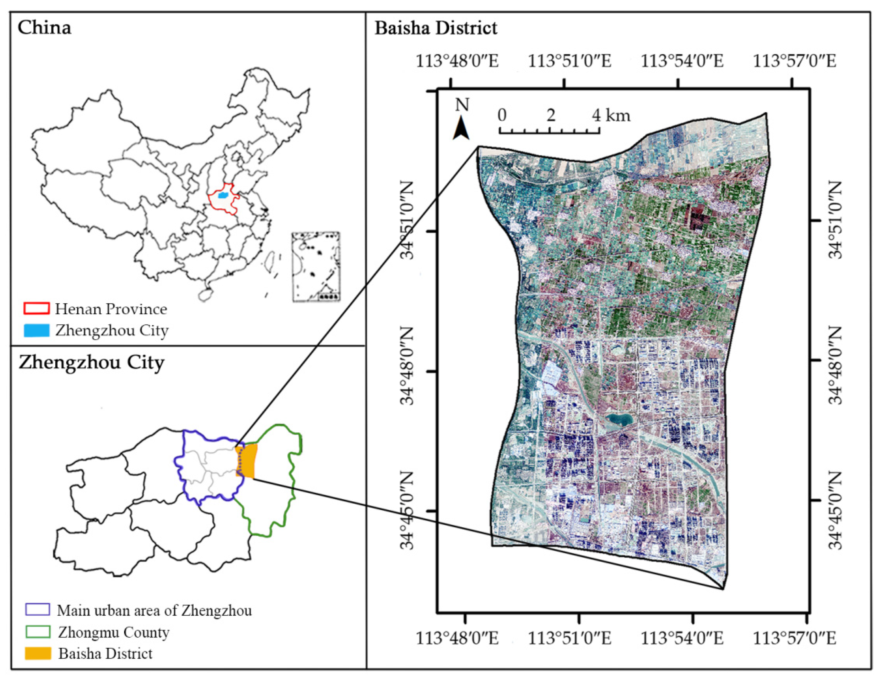
2.1. Study Area

Baisha District belongs to the peri-urban region located next to the core area of Zhengzhou (34°43′–34°54′ N, 113°49′–113°56′ E) (Figure 1). With the development of the Central Plains urban agglomeration and the Zhengzhou metropolitan area, it continues to experience urbanization. Its planning scope begins from the Beijing–Hong Kong–Macao Expressway in the west to the New 107 National Road in the east, and from the Zhengzhou City boundary of the Yellow River in the north to the Longhai Railway in the south, with a total area of 156 km2. It belongs to the Huanghuai Plain with warm temperate continental monsoon climate. Water resources are relatively abundant and there are many large water areas such as the Jialu River and Xianghu Lake. There are ecological corridors and the natural conditions are superior. Considering the study area is adjacent to the central urban area of Zhengzhou in the east and Bianxi New District of Kaifeng in the west, its transportation has been greatly improved under the integrated development of Zhengzhou–Kaifeng, which can realize three-dimensional docking and one-stop transfer with Zhengzhou’s high-speed railway station and subway station; as many main roads run through it, it combines the advantages of train, bus, and plane transportation.

2.2. Remote Sensing Data of GI

The data used in this research were derived from Google Earth remote sensing images captured in 2007, 2013, and 2018 that were of good quality and free of clouds. Standard radiometric and geometric corrections were implemented.
The extraction and classification process of GI were completed by the eCognition9.0 software: first, we sequentially used “multi-scale segmentation” and “spectral difference segmentation” to divide the remote sensing images into multiple objects. Next, based on the identification feature information (e.g., spectrum, geometry, texture, and topology) of each object, we conducted the membership function classification and nearest neighbor classification in turn, after which the GI in the study area were identified. According to the classification results, we manually examined and corrected any visible classification errors. Lastly, to validate the precision, we applied a simple random sampling method that compared the reference points selected randomly from the classification results to the corresponding points from the Google Earth imagery [40]. The final overall accuracies were over 85%.
Researchers have emphasized that the ambiguous definition of GI has generated a high diversity in research objectives and outputs [41], and at present, there is no consensus on a comprehensive classification for GI [42]. Considering the study purposes, scales, and imageries adopted in this paper, the GI classification was formulated based on the existing classification mentioned [36] that includes farmland, greenspace, water area, and forestland (Table 1).

2.3. Landscape Pattern Index

The landscape pattern index provides an effective method for the quantitative analysis of landscape spatial patterns [28]. To accurately demonstrate the dynamics of GI in the study area in terms of quantity, shape, and agglomeration characteristics, this study selected six representative landscape pattern indices with low redundancy based on relevant studies [43] (Table 2): Percentage of Landscape (PLAND), Largest Patch Index (LPI), Fractal Dimension Index (FRAC_MN), Landscape Shape Index (LSI), Patch Density (PD), and Patch Cohesion Index (COHESION). Of these, PLAND and LPI were selected to reflect quantitative characteristics of GI from the aspects of patch area percentage and advantage proportion, respectively; FRAC_MN and LSI were selected to jointly reflect the complexity of landscape shape; and PD and COHESION were selected to reflect the aggregation characteristics of GI from the perspective of patch fragmentation and connectivity. Through the comprehensive analysis of these six indices, the spatial pattern of the GI in Baisha District can be determined in detail and dynamic research can be conducted. The calculation of the landscape indices used were all conducted using the Fragstats 4.2 software.

2.4. Spatial Autocorrelation Analysis

Spatial autocorrelation analysis can present the spatial properties of the GI through quantitative and visual methods, and it is performed using two key indicators: Global Moran’s I and LISA (the local indicators of spatial association) [49]. Global Moran’s I reflects the presence or absence of spatial autocorrelation as a whole, while LISA measures the local patterns of spatial association and the distribution state of local heterogeneity by using local Moran’s I [38,50].
The equation for Global Moran’s I is:
I = i = 1 n j = 1 n w i j ( x i x ¯ ) ( x j x ¯ ) / S 2 i = 1 n j = 1 n w i j ,
S 2 = 1 n j ( x i x ¯ ) 2 ,
The expression for LISA is:
I i = ( x i x ¯ ) S 2 j w i j ( x j x ¯ ) ,
where I is the Moran’s I index; n is the total number of spatial units; x and x ¯ denote the values of the variable elements and their averages; and wij is the spatial weight, constructed based on the queen criterion of contiguity in this paper. I ranges from −1 to +1 and when the value is closer to 1, regions with similar attributes are more clustered together (high-high cluster or low-low cluster). Conversely, when the value is closer to −1, regions with distinct properties are more closely aggregated (high-low outlier or low-high outlier) [38].
The calculation of Moran’s I is based on the identification of neighborhoods which are defined by a grid scale [51]. A grid scale of 1.0 km × 1.0 km (a grid structure with sides of length 1.0 km) is usually applied to the ecological environment assessment, land use change research, and simulation of the spatial distribution of variables [52,53]; considering it can better distinguish various landscape types in Baisha District, this paper selected 1.0 km × 1.0 km as the basic research scale. In addition, to avoid the impact of grid size on the comparison results, we expanded and contracted the basic scale to grid scales of 1.5 km × 1.5 km, 0.5 km × 0.5 km; then, we calculated the six landscape indices for each local spatial unit and, finally, further analyzed the spatial autocorrelation of GI characteristics on the three grid scales. The calculation and inspection of Global Moran’s I and the LISA clustering map were realized by GeoDa software (GeoDa Center for Geospatial Analysis and Computation, 2015).

3. Results

3.1. Total Trends

From 2007 to 2018, the coverage of GI decreased dramatically, especially for the southern farmland (Figure 2). The PLAND decreased drastically from 88.61% to 68.82% and the LPI was greatly reduced from 26.92% to 6.18% (Table 3), indicating that the area of the total GI and the largest GI patch had diminished significantly. Additionally, the COHESION was also reduced from 99.97to 99.81. In contrast, the LSI gradually increased from 29.83 in 2007 to 57.43 in 2018, reflecting that the landscape patches became more complicated. Both FRAC_MN and PD recorded maxima (1.23, 37.37 patchs·100 hm−3) in 2013 and minima (1.18, 19.05 patchs·100 hm−3) in 2018, indicating that the GI had the most complex patch shape and highest fragmentation in 2013, and the simplest patch shape and lowest fragmentation in 2018.

3.2. Class-Level Trends

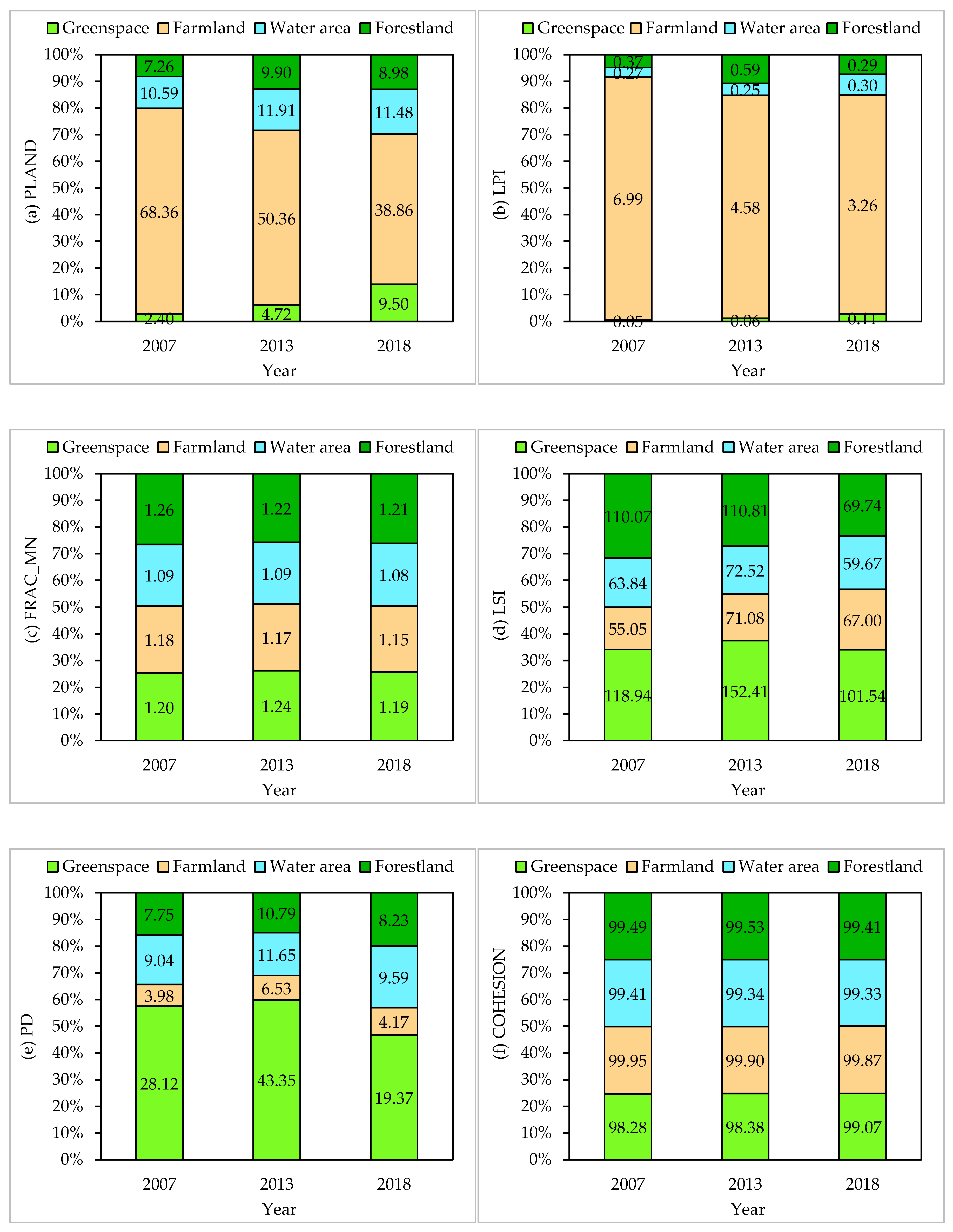
3.2.1. Landscape Pattern Index Variation

From 2007 to 2018, the PLAND, LPI, and COHESION of farmland all decreased constantly (Figure 3). Although its PLAND slumped from 68.36% to 38.86%, LPI reduced from 6.99% to 3.26% and COHESION decreased from 99.95 to 99.87; these values were consistently higher than those for other types, indicating that farmland was the dominant GI with the highest landscape composition and connectivity. Conversely, the PLAND, LPI, and COHESION of greenspace increased progressively; while the greenspace PLAND was the smallest in 2007–2013, its LPI and COHESION continued to be at the minimum for GI. Additionally, forestland made up the smallest proportion (8.98%) of GI in 2018 and its PLAND, LPI, and COHESION showed a similar trend of increasing (2007–2013) initially and then decreasing (2013–2018).
The FRAC_MN of different types of GI in 2018 were all smaller than in 2007; the FRAC_MN of the water area was consistently lower than that of the other GI, indicating that the shapes of different GI became simpler, and the water area maintained the most regular shape. Additionally, the PD and LSI of different GI reached their maximum in 2013. The PD and LSI of greenspace were much higher than those of other GI in 2007–2018, indicating that the landscape patches of different GI were the most complex and fragmented in 2013. In particular, greenspace showed the most prominent performance during the study period.

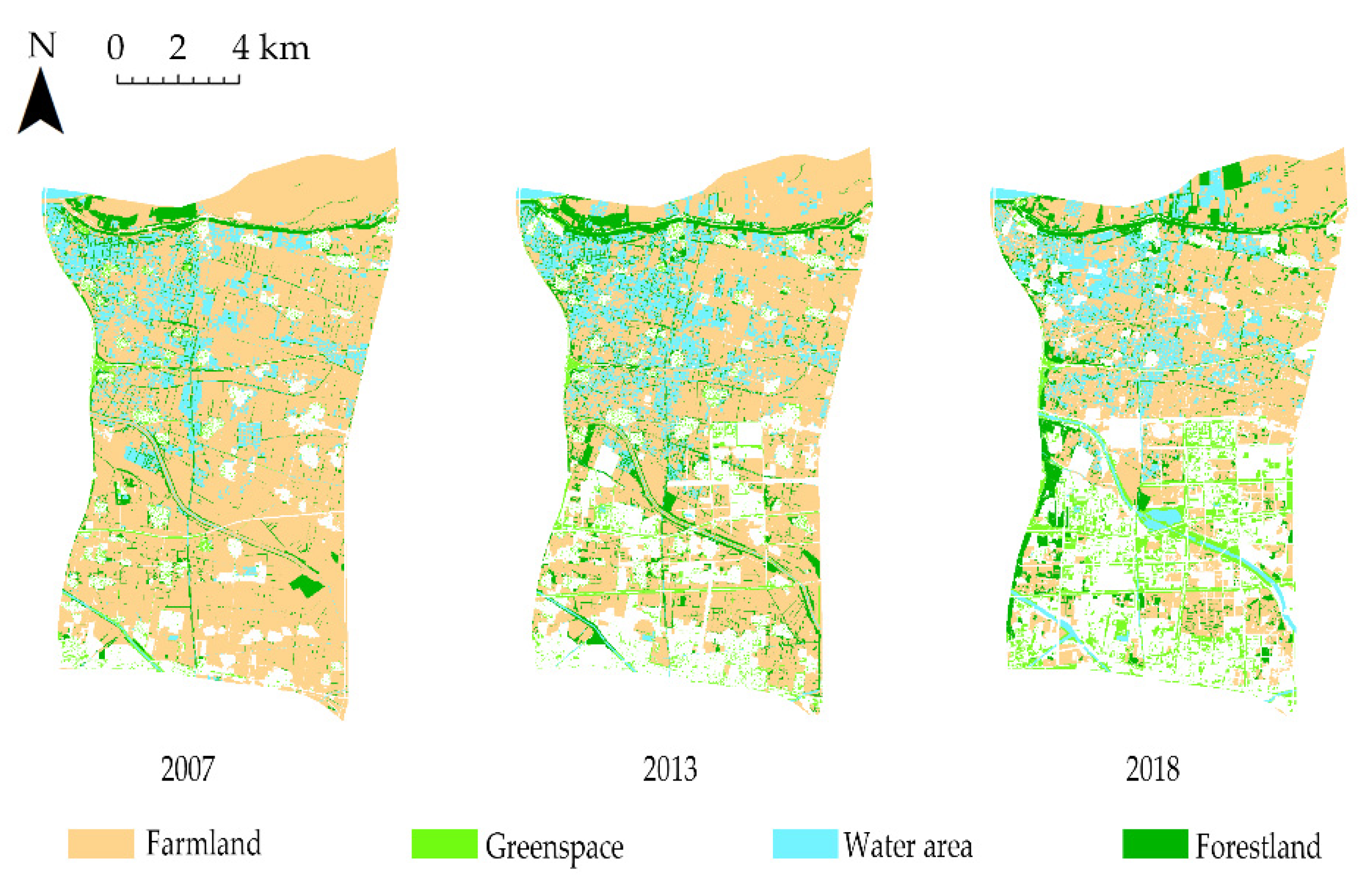
3.2.2. Mutual Transformation in GI

The main sources of the new areas of greenspace, forestland, and water areas were farmland, and the total areas of farmland converted into other GI were 19.92 km2, 16.82 km2, and 28.61 km2 in 2007–2013, 2013–2018, and 2007–2018 (Table 4, Table 5 and Table 6), respectively, far higher than the greenspace, forestland, and water areas. In 2007–2013 and 2013–2018, farmland was mainly transformed into forestland with the conversion area being 8.63 km2 and 6.88 km2 respectively, while in 2007–2018, farmland was mainly converted to greenspace (9.68 km2), followed by forestland (9.57 km2). This was related to the transfer of more forestland to other GI. From the perspective of net growth, only farmland exhibited a net transfer out, while all other GI exhibited a net transfer in, as the net increase of the water area ranked lowest in 2007–2013 (2.98 km2) and 2013–2018 (0.38 km2). Specifically, forestland had the largest net increase in 2007–2013 (5.26 km2), while greenspace had the largest net increase in 2013–2018 (4.95 km2).

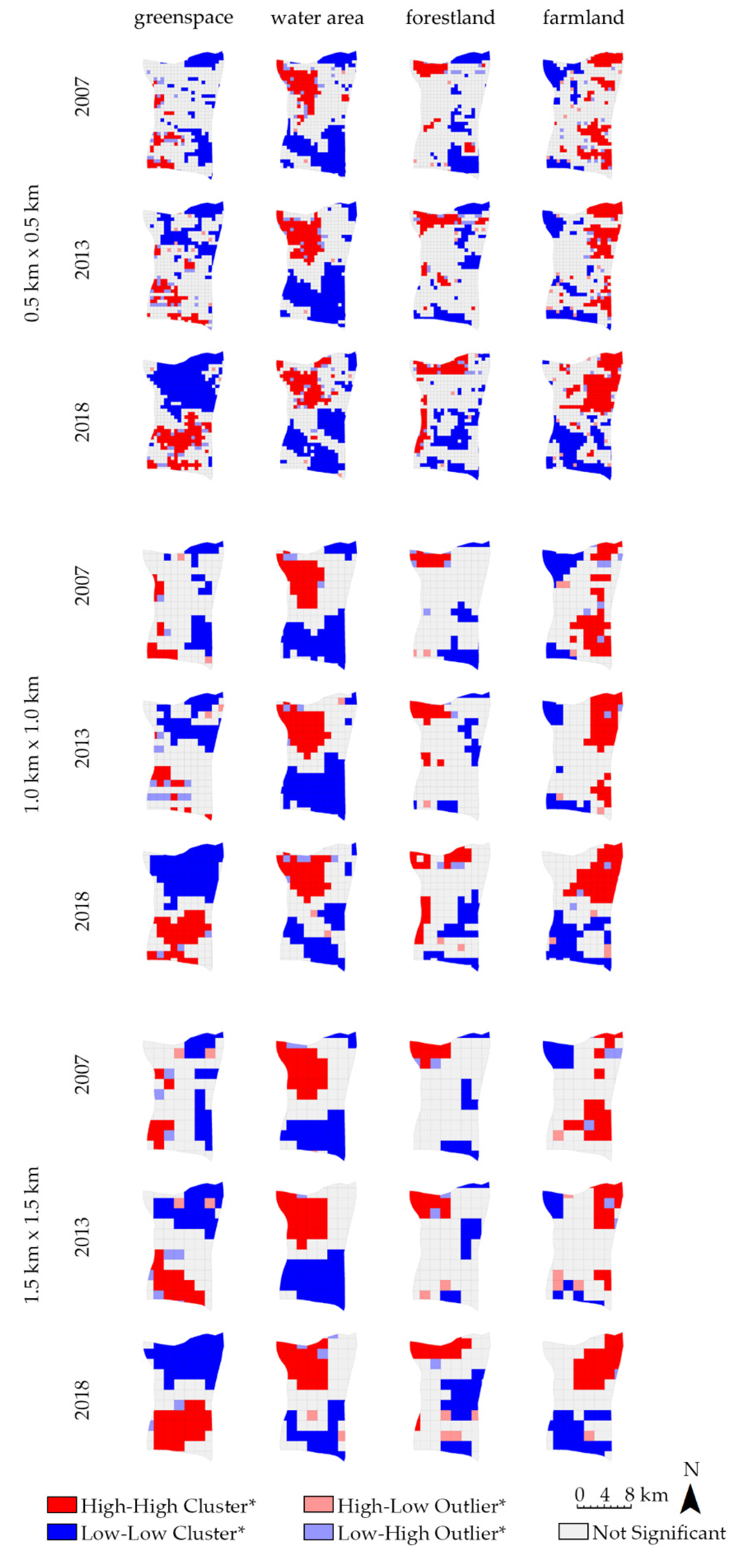
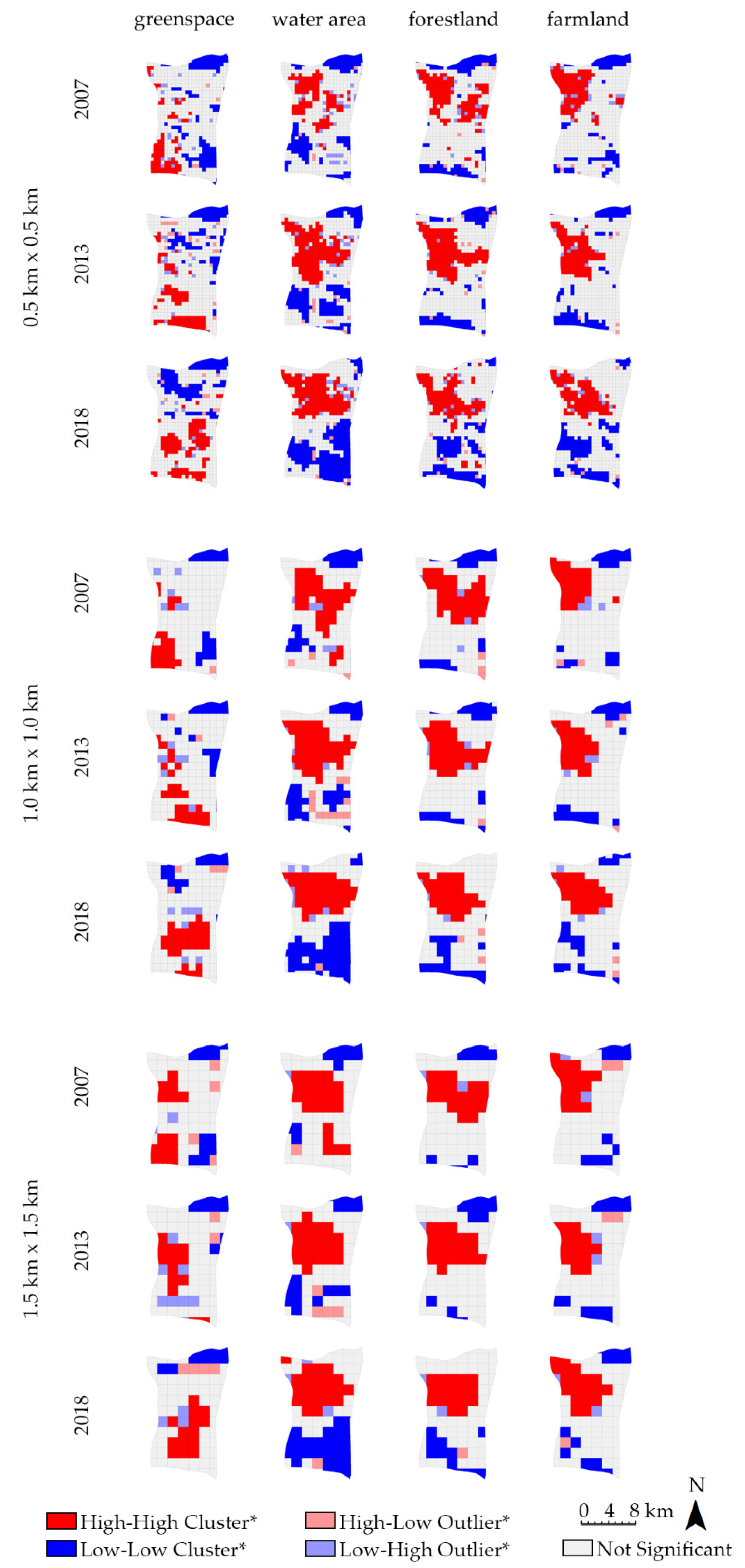
3.3. Spatial Autocorrelation Analysis

3.3.1. Changes in Spatial Agglomeration Effects

Except for the water area FRAC_MN (−0.02, 1.5 km × 1.5 km, 2013), the Global Moran’s I for other indices at each scale were all greater than 0 (Figure 4), indicating that the corresponding landscape pattern features had different spatial agglomeration effects (p < 0.001). For greenspace, farmland, and forestland, the Global Moran’s I of PLAND were all enhanced in 2013–2018, indicating that their spatial aggregation characteristics increased during this period. Additionally, the Global Moran’s I of their PD in 2018 were higher than 2007, showing the enhanced spatial aggregation distribution of their landscape fragmentation. Moreover, the Global Moran’s I of greenspace COHESION increased over time at the three scales, showing that the connectivity of greenspace became more aggregated in the spatial distribution during the study period.
The Global Moran’s I of PD for farmland and water area on the 0.5 km grid scale were all close to 0 and the Global Moran’s I of water area FRAC_MN was −0.02 in 2013 on the 1.5 km grid scale, indicating that their corresponding landscape features were close to random distributions. Moreover, the Global Moran’s I of PLAND was generally higher than that of LPI which indicated that PLAND displayed a more prominent spatial aggregation. Therefore, we selected PLAND, LSI, and COHESION, which had relatively higher Global Moran’s I at the three scales, to analyze the local spatial autocorrelation in terms of quantity, shape, and agglomeration characteristics, and to further explore the spatial aggregation distribution changes in GI.
Figure 5, Figure 6 and Figure 7 show that the local patterns of spatial association for GI features at the three scales were dominated by high-high and low-low clusters, while high-low and low-high outliers were very rare. In 2007, high-high clusters of farmland PLAND were distributed in the east, while they were gradually reduced in the south and expanded in the north in 2013. By 2018, a distinct north–south difference had formed: the high-high clusters were mainly concentrated in the north while the low-low clusters were primarily distributed in the south. Additionally, the high-high clusters of farmland LSI mainly distributed in the northwest region in 2007–2018, while the high-high clusters of farmland COHESION gradually concentrated in the northeast region, demonstrating that high-value farmland gradually gathered in the north; the connectivity of farmland in the northeast region was relatively higher; and the shape of farmland in the northwest region was relatively complicated and fragmented. For greenspace, the high-high clusters of PLAND, LSI, and COHESION were concentrated mainly on the southwestern area, followed by the western region in 2007; they gradually moved to the south over time and by 2018, the clustering features had formed a clear north–south divide with the difference in farmland being that the high-high clusters were mainly concentrated in the south and the low-low clusters were primarily spread in the north, demonstrating that the high-value greenspace was mainly concentrated in the south with high connectivity and complex patch shapes. In terms of the water area and forestland, high values of PLAND, LSI, and COHESION were clustered mainly in the north, while low-value aggregation areas were primarily distributed in the south in 2007–2018.

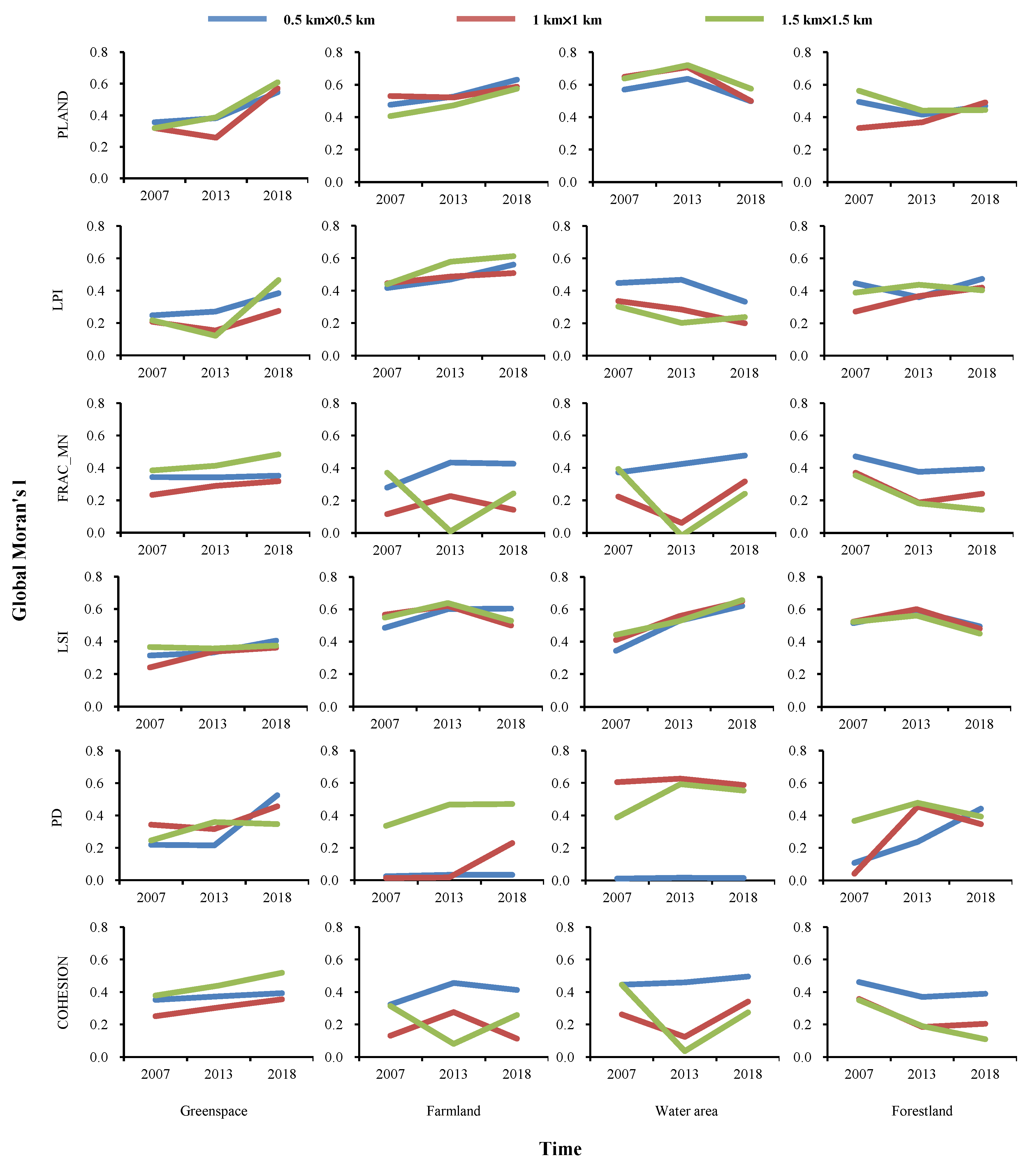
3.3.2. Scale Effects

On the three scales of observation, the proportion of high-high clusters of forestland PLAND and greenspace COHESION increased continuously over time (Figure 8), indicating that the area of forestland and the connectivity of greenspace all improved in 2007–2018, and that the ecological policies such as reforestation and greenspace system planning achieved certain results. However, the proportions of low-low clusters of PLAND in greenspace, water area, and forestland were higher than those of high-high clusters, indicating that their spatial distribution was still dominated by low-value clusters. Thus, the development of greenspace, water areas, and forestlands needs to be further improved.
In 2018, the proportion of high-high clusters of PLAND and COHESION in greenspace decreased with the reduction of scale, indicating that greenspace was less distributed and had lower connectivity on the 0.5 km grid scale. In addition, the percentage of high-high clusters of water area PLAND also decreased as the spatial scale shrunk. It is therefore necessary to enhance the greenspace and water area at the smaller scale (0.5 km × 0.5 km) as increasing street trees, community green areas, and water bodies of parks and improving the connectivity between them can effectively change the current situation. For farmland, the percentage of high-high clusters of PLAND and COHESION in 2018 decreased with the increase of scale, while the percentage of high-high clusters of LSI behaved contrarily; in addition, the percentage of low-low clusters of PLAND increased by 14% on the 1.5 km grid scale and the percentage of high-high clusters increased by 5% on the 0.5 km grid scale. The above indicates serious encroachments on farmland on the scale of 1.5 km grid with a more complicated shape and the high-values of area and connectivity were more clustered on the smaller scale. Therefore, in the protection of farmland, it is necessary to avoid further increase of low-value aggregation areas on the 1.5 km grid scale and to protect the high-value aggregation areas on the 0.5 km grid scale from being destroyed.

4. Discussion

4.1. Spatiotemporal Dynamics of GI

The total GI in Baisha District decreased dramatically from 88.61% to 68.82% and its largest patch proportion declined remarkably from 26.92% to 6.18% in 2007–2018. This indicates that the GI in the agricultural peri-urban area between Zhengzhou and Kaifeng was drastically reduced in the process of urban integration and large areas of intact GI have been eroded to make way for buildings, roads, and other gray infrastructures. Similar findings have been confirmed in Australia [54], Dhaka [27], Addis Ababa, and Dar es Salaam [55]. Additionally, we found that the spatiotemporal variation of different GI in Baisha and their impact on the overall GI were different. The farmland was the dominant GI and had the highest connectivity, although its percentage decreased drastically from 68.36% to 38.86% in 2007–2018 and its spatial distribution tended to be intensive (high values gradually concentrated in the north). These are typical features in the change of suburban farmland against the background of urbanization and have been confirmed in the research of Colantoni [56], Lee [31], and Yu [57] on farmland in the peri-urban areas. For the greenspace, although its proportion increased and the landscape connectivity improved, it still recorded the most complex shape, the greatest fragmented patches, and the lowest landscape connectivity from 2007 to 2018. It is noteworthy that greenspace PD and its variation were far higher than those of the other types in the same period, reflecting that the fragmentation of GI in Baisha District depended on greenspace to some extent. Moreover, the agricultural peri-urban area has often not formed a complete GI system, unlike the city center [58], as we found that the high-connectivity clusters for farmland, water areas, and forestland are concentrated in the north, while low-connectivity clusters are distributed in the south.

4.2. Driving Policies in GI Dynamics

Studies have shown that although population migration, climate, latitude, and other factors affect the change of GI to a certain extent, policies are the major driving forces. Byomkesh [27] found that the drastic reduction of green spaces in Greater Dhaka can be attributed to a lack of policy, low political motivation, and poor management. Wu [22] found that greening policies are major driving factors of changes in green spaces in Shanghai. Hersperger [59] found that political driving forces contributed to 26% of landscape change and variations in the agricultural and forestry network, and the loss of elements of the traditional agricultural landscape and new solitary trees have been associated with political driving forces. Moreover, Fan [60] explained that the government planning area was different from watershed and administrative regions, and its landscape changes can directly reflect the impact of policies. In this study of Baisha District, the government planning area, GI had undergone tremendous changes driven by a series of policies from 2007–2018, although it is located in the agricultural peri-urban area.
At the national level, the concepts of “Ecological Civilization”, “Green Development”, “Eco-City”, and “Ecological Red Line” emphasized by the Chinese central government provide national policy guarantees for the sustainable development of GI [22]. Under these frameworks, the governments of Henan Province and Zhengzhou City have initiated policies and measures to maintain a balance between urbanization and GI development. In 2007, the Outline of the Overall Development Plan for the Central Henan Urban Agglomeration [61] entered the implementation stage, requiring the integrated areas of Zhengzhou–Kaifeng to build green corridors on both sides of the main roads, to build ecological regulation areas of forest and green space in feasible areas, and to develop urban and sightseeing agriculture so as to realize ecological docking. Furthermore, the Master Plan for the Area along Zhengzhou–Kaifeng Avenue also proposed the construction of a “ring, belt, and point” green space system. “Ring” refers to the ecological protection ring surrounding the area and is mainly composed of shelterbelts and basic farmland; “belt” refers to the greening or ecological isolation belts which are mainly composed of urban agricultural areas, green belts, and major water systems; and “point” refers to various urban parks and street green spaces distributed within the area [62]. From 2007 to 2018, the Zhengzhou Municipal Government successively implemented the Zhengzhou City Master Plan (2010–2020), Zhengzhou City Green Space System Plan (2013–2030), Zhengzhou National Central City Ecological Construction Plan (2016–2025), Zhengzhou Forestry Ecological Construction Implementation Plan (2017), and Zhengzhou City Ecological Protection and Construction Plan (2017–2035) concerning, respectively, the construction of the Ecological Cultural Tourism Industrial Belt along the Yellow River [63], Ecological Belt along the Yellow River in Northern Zhengzhou [64], Ecological Wetland Landscape Belt along the Yellow River, Ecological Barrier Zone along the Yellow River in Northern Zhengzhou [65], and the Yellow River Ecological Conservation and Ecological Cultural Development Zone. These initiatives entail returning farmland to forests and wetlands, widening and thickening the protective forest belt along the embankments and connecting water systems, and implementing ecological water replenishment and other measures to gradually improve the GI of the Yellow River basin, with “Wetland-Shelter Forest-Ecological Farmland” as the leading factor. These policies have greatly promoted the development of farmland, water areas, and forestland in the northern part of the study area which belongs to the Yellow River Basin. They are also the reason why the high-high clusters of farmland PLAND and COHESION have gradually moved to the north on the three scales, gathering in the north similar to water areas and forestland in 2018.
The Master Plan for the Baisha District in Zhengdong New District, Zhengzhou (2013–2030) positioned the research area as a provincial administrative center and the central area is located in Xiang Lake in the southern part of Baisha [64]. With the thorough implementation of this plan, the construction of gray infrastructure such as buildings and roads in the southern area has been continuously strengthened as the population has continued to gather in the south and greenspace such as community gardens, street trees, and parks are also increasing. Therefore, the values of PLAND, LSI, and COHESION for greenspace have gradually increased and their high-high clusters gradually moved to the south from 2007 to 2018.

4.3. Implications for the Future

4.3.1. Ensuring the Dominant Position of Farmland and Achieving Its High-Quality Development

Farmland plays an important role in food supply, rain and flood regulation, and groundwater replenishment [31,66]. As the dominant GI, its sustainable development is crucial for agricultural peri-urban areas. Given the substantial reduction of farmland in Baisha District and the high-high clusters of farmland PLAND gradually gathering in the north, the north must improve and refine the basic farmland protection system and strictly prohibit the unrestricted expansion of buildings and roads to maintain the integrity of farmland ecosystem services. Moreover, considering the high-high clusters of farmland LSI are mainly distributed in the northwest region in 2007–2018, it is necessary to reduce the complexity of the shape of the farmland in the northwest region to improve its connectivity. Additionally, we found that the farmland had been seriously encroached upon on the 1.5 km grid scale, its shape was more complicated, and the high-value of area and connectivity were more clustered on the smaller scale. It is therefore crucial that further increases of low-value aggregation areas on the 1.5 km grid scale be avoided and that high-value aggregation areas on the 0.5 km grid scale be protected from being destroyed. To achieve high-quality development of farmland, its park-type transformation, and the transformation and upgradation of traditional agriculture to leisure sightseeing agriculture can be promoted, which is conducive to the formation of a comprehensive GI system among farmlands, forestlands, greenspaces, and water areas, yielding a higher ecosystem service value. Moreover, there is an opportunity for the northern farmland to be further combined with the national strategy of ecological protection and high-quality development of the Yellow River basin, as well as an opportunity to increase the interaction between farmland and other GI along the Yellow River, providing a solid foundation for the formation of high-quality ecological space in the study area.

4.3.2. Reducing the Fragmentation of Greenspace

It is noteworthy that greenspace PD and its variation were far greater than those of other GI throughout the study period. The proportion of high-high clusters of greenspace PLAND and COHESION decreased with the reduction of scale in 2018; therefore, the greenspace fragmentation, especially in the southern region in which the high-high clusters of greenspace PLAND, LSI, and COHESION were mainly concentrated, must be urgently reduced. Considering that there is a higher population density and more buildings and roads in the south, various types and functions of greenspace can be increased such as street trees, parks, community gardens, rooftop gardens, and ecological corridors, enabling the connection of fragmented greenspaces at the smaller scale (0.5 km × 0.5 km). Additionally, considering the north is a low-value aggregation area of greenspace PLAND, promoting connections of farmland, forestland, and water areas by increasing northern greenspace can be considered in order to form a comprehensive GI system.

4.3.3. Enhancing the Development of Forestland and Water Areas

Forestland comprises the smallest proportion (8.98%) of GI in 2018 and the net increase of water areas consistently ranked lowest in both 2007–2013 (2.98 km2) and 2013–2018 (0.38 km2); therefore, it is important to enhance the development of forestlands and water areas, especially in the southern region, in which the low-low clusters of forestland and water areas are primarily distributed. It would be effective to add windbreaks, forest parks, and the protection forestlands of roads in the south. Moreover, considering the percentage of high-high clusters of water area PLAND decreased as the spatial scale shrank, it is also necessary to enhance the water area at the smaller scale (0.5 km × 0.5 km) as increasing the water space of parks and communities and increasing the connectivity between them can effectively change the current situation. Meanwhile, it is important to enhance the development of larger water areas such as Xianghu Lake, Jalu River, and the Dongfeng Canal to safeguard their higher ecological service functions.

4.4. Limitation

Several limitations in this paper should be acknowledged. Firstly, subject to the classification techniques, the category of GI was comparatively rough. Secondly, a relatively low number of landscape pattern indices and grid scales were selected. In the future, the greater subdivision of GI, continuous grid scales, and extensive evaluation indicator systems should be considered as comprehensive as possible for assessment.

5. Conclusions

Based on three-phase remote sensing data, this paper investigated the spatiotemporal dynamics of GI in Baisha District from 2007 to 2018. The results demonstrated the following: (1) The total GI had a continuing downward trend in the proportion, dominant patch area ratio, and entire connectivity. (2) Farmland was the dominant GI, although its percentage decreased drastically from 68.36% to 38.86%, and farmland was partly converted to greenspace, forestland, and water areas. Greenspace was the main type that led to fragmentation, although its proportion and connectivity improved. (3) Spatially, the high-value clusters of farmland and forestland gradually concentrated in the north, and the low-value clusters moved to the south, while greenspace showed the opposite tendency; the high-value clusters of water areas were concentrated on both sides of the Jialu River in the northwest. Low-value clusters were located in the southeast. (4) The shape of greenspace and forestland patches became more regular, and the shape of water areas and farmland patches became more natural in northwest, while more regular in southeast.
The study contributed to a better understanding of the dynamics of the GI spatiotemporal patterns in agricultural peri-urban areas and had important enlightenment outcomes for planning and management policies for Baisha District and other agricultural peri-urban areas: (1) Ensuring the dominant position of farmland is critical for maintaining the composition and connectivity of the overall GI. Farmland and fish pond patch clusters should be protected to ensure food security; however, the recreation, inheritance of farming culture, and ecosystem service functions of farmland should be improved to meet the growing needs of urban residents. (2) According to the perspective of ecological security, the Baisha District in this study is located in the downstream of Zhengzhou City with a lower terrain than the main urban area. GI includes the farmlands, greenspace, and wetlands on both sides of the Jialu River that should be retained and restored as much as possible to protect natural ecological process. Simultaneously, the construction of important urban facilities and residential areas in flooded areas should be banned. (3) Due to policy of urban greenspace planning, urban greenspace is becoming more fragmented and the shape tends to be more regular. A part of the evenly distributed large greenspace patches should be moved to both sides of the Jialu River to increase the agglomeration effect of GI.

Author Contributions

Conceptualization, H.X. and Y.L. (Yakai Lei); data curation, H.X.; formal analysis, G.K.; funding acquisition, Y.L. (Yakai Lei); investigation, H.X.; methodology, H.X. and S.G.; project administration, Y.L. (Yakai Lei); resources, Y.L. (Yakai Lei); software, H.X.; supervision, G.K. and Y.L. (Yang Liu); validation, G.K.; visualization, H.X. and X.Z.; writing—original draft, H.X.; writing—review and editing, H.X., G.K., and Y.L. (Yakai Lei). All authors have read and agreed to the published version of the manuscript.

Funding

This research was funded by the National Natural Science Foundation of China, grant number 31600579, and the Key Technology Program of Henan Province, grant number 162102310093.

Data Availability Statement

The data presented in this study are available on request from the first author.

Acknowledgments

The authors would like to thank the support of the International Joint Laboratory of Landscape Architecture, Henan Agricultural University, for their infinite help.

Conflicts of Interest

The authors declare no conflict of interest.

References

  1. McIntyre, N.E.; Knowles-Yánez, K.; Hope, D. Urban ecology as an interdisciplinary field: Differences in the use of urban between the social and natural sciences. Urban Ecosyst. 2000, 4, 5–24. [Google Scholar] [CrossRef]
  2. Grimm, N.B.; Faeth, S.H.; Golubiewski, N.E.; Redman, C.L.; Wu, J.; Bai, X.; Briggs, J.M. Global change and the ecology of cities. Science 2008, 319, 756–760. [Google Scholar] [CrossRef] [PubMed] [Green Version]
  3. Ge, S.; Zhao, S. Organic Carbon Storage Change in China’s Urban Landfills from 1978–2014. Environ. Res. Lett. 2017, 12, 104013. [Google Scholar] [CrossRef]
  4. Zhao, S.; Liu, S.; Zhou, D. Prevalent vegetation growth enhancement in urban environment. Proc. Natl. Acad. Sci. USA 2016, 113, 6313–6318. [Google Scholar] [CrossRef] [Green Version]
  5. World Urbanization Prospects: 2018 Revision. 2018. Available online: https://data.worldbank.org/indicator/SP.URB.TOTL.IN.ZS (accessed on 30 July 2018).
  6. Fang, C.; Yu, D. Urban agglomeration: An evolving concept of an emerging phenomenon. Landsc. Urban Plan. 2017, 162, 126–136. [Google Scholar] [CrossRef]
  7. Fang, C. Important progress and future direction of studies on China’s urban agglomerations. J. Geogr. Sci. 2015, 25, 1003–1024. [Google Scholar] [CrossRef] [Green Version]
  8. Mortoja, M.G.; Yigitcanlar, T.; Mayere, S. What is the most suitable methodological approach to demarcate peri-urban areas? A systematic review of the literature. Land Use Policy 2020, 95, 104601. [Google Scholar] [CrossRef]
  9. Rahman, M.T.; Aldosary, A.S.; Mortoja, M.G. Modeling future land cover changes and their effects on the land surface temperatures in the Saudi Arabian eastern coastal city of Dammam. Land 2017, 6, 36. [Google Scholar] [CrossRef]
  10. Roose, A.; Kull, A.; Gauk, M.; Tali, T. Land use policy shocks in the post-communist urban fringe: A case study of Estonia. Land Use Policy 2013, 30, 76–83. [Google Scholar] [CrossRef]
  11. Zhu, F.; Zhang, F.; Ke, X. Rural industrial restructuring in China’s metropolitan suburbs: Evidence from the land use transition of rural enterprises in suburban Beijing. Land Use Policy 2018, 74, 121–129. [Google Scholar] [CrossRef]
  12. Sanesi, G.; Colangelo, G.; Lafortezza, R.; Calvo, E.; Davies, C. Urban green infrastructure and urban forests: A case study of the Metropolitan Area of Milan. Landsc. Res. 2017, 42, 164–175. [Google Scholar] [CrossRef]
  13. Hernández-Moreno, Á.; Reyes-Paecke, S. The effects of urban expansion on green infrastructure along an extended latitudinal gradient (23° S–45° S) in Chile over the last thirty years. Land Use Policy 2018, 79, 725–733. [Google Scholar] [CrossRef]
  14. Anders, W.; Zhang, Q. Reclaiming localisation for revitalising agriculture: A case study of peri-urban agricultural change in Gothenburg, Sweden. J. Rural. Stud. 2016, 47, 172–185. [Google Scholar]
  15. Afriyie, K.; Abas, K.; Adomako, J.A.A. Urbanisation of the rural landscape: Assessing the effects in peri-urban Kumasi. Int. J. Urban Sustain. Dev. 2014, 6, 1–19. [Google Scholar] [CrossRef]
  16. Nigussie, S.; Li, L.; Yeshitela, K. Towards improving food insecurity in urban and peri-urban areas in Ethiopia through map analysis for planning. Urban For. Urban Green. 2021, 58, 126967. [Google Scholar] [CrossRef]
  17. Khushbu, K.B.; Hymavathi, T.; Mathuvanthi, C.N.; Mayaja, N.A.; Srinivasa, C.V. Impact of urbanisation on lakes-a study of Bengaluru lakes through water quality index (WQI) and overall index of pollution (OIP). Environ. Monit. Assess. 2021, 193, 408. [Google Scholar]
  18. Huang, C.; Huang, P.; Wang, X.; Zhou, Z. Assessment and optimization of green space for urban transformation in resources-based city—A case study of Lengshuijiang city, China. Urban For. Urban Green. 2018, 30, 295–306. [Google Scholar] [CrossRef]
  19. Semeraro, T.; Aretano, R.; Pomes, A. Green infrastructure to improve ecosystem services in the landscape urban regeneration. IOP Conf. Ser. Mater. Sci. Eng. 2017, 245, 082044. [Google Scholar] [CrossRef]
  20. Kim, J.H.; Jobbágy, E.G.; Jackson, R.B. Trade-offs in water and carbon ecosystem services with land-use changes in grasslands. Ecol. Appl. 2016, 26, 1633–1644. [Google Scholar] [CrossRef] [Green Version]
  21. Knoke, T.; Paul, C.; Hildebrandt, P.; Calvas, B.; Castro, L.M.; Härtl, F.; Döllerer, M.; Hamer, U.; Windhorst, D.; Wiersma, Y.F.; et al. Compositional diversity of rehabilitated tropical lands supports multiple ecosystem services and buffers uncertainties. Nat. Commun. 2016, 7, 11877. [Google Scholar] [CrossRef] [PubMed]
  22. Wu, Z.; Chen, R.; Meadows, M.E.; Sengupta, D.; Xu, D. Changing urban green spaces in Shanghai: Trends, drivers and policy implications. Land Use Policy 2019, 87, 104080. [Google Scholar] [CrossRef]
  23. Roces-Díaz, J.V.; Vayreda, J.; Banqué-Casanovas, M.; Díaz-Varela, E.; Bonet, J.A.; Brotons, L.; de-Miguel, S.; Herrando, S.; Martínez-Vilalta, J. The spatial level of analysis affects the patterns of forest ecosystem services supply and their relationships. Sci. Total Environ. 2018, 626, 1270–1283. [Google Scholar] [CrossRef] [PubMed] [Green Version]
  24. Duy Thinh, D.; Huang, J.; Cheng, Y.; Thi Cat Tuong, T. Da Nang green space system planning: An ecology landscape approach. Sustainability 2018, 10, 3506. [Google Scholar]
  25. Liu, W.; Holst, J.; Yu, Z. Thresholds of landscape change: A new tool to manage green infrastructure and social-economic development. Landsc. Ecol. 2014, 29, 729–743. [Google Scholar] [CrossRef]
  26. Qian, Y.; Zhou, W.; Li, W.; Han, L. Understanding the dynamic of greenspace in the urbanized area of Beijing based on high resolution satellite images. Urban For. Urban Green. 2015, 14, 39–47. [Google Scholar] [CrossRef]
  27. Byomkesh, T.; Nakagoshi, N.; Dewan, A.M. Urbanization and green space dynamics in Greater Dhaka, Bangladesh. Landsc. Ecol. Eng. 2012, 8, 45–58. [Google Scholar] [CrossRef]
  28. Su, S.; Wang, Y.; Luo, F.; Mai, G.; Pu, J. Peri-urban vegetated landscape pattern changes in relation to socioeconomic development. Ecol. Indic. 2014, 46, 477–486. [Google Scholar] [CrossRef]
  29. Sharp, J.S.; Clark, J.K. Between the country and the concrete: Rediscovering the rural-urban fringe. City Community 2008, 7, 61–79. [Google Scholar] [CrossRef]
  30. Huang, S.-L.; Lee, Y.-C.; Budd, W.W.; Yang, M.-C. Analysis of changes in farm pond network connectivity in the peri-urban landscape of the Taoyuan area, Taiwan. Environ. Manag. 2012, 49, 915–928. [Google Scholar] [CrossRef]
  31. Lee, Y.-C.; Ahern, J.; Yeh, C.-T. Ecosystem services in peri-urban landscapes: The effects of agricultural landscape change on ecosystem services in Taiwan’s western coastal plain. Landsc. Urban Plan. 2015, 139, 137–148. [Google Scholar] [CrossRef]
  32. Kar, R.; Obi Reddy, G.P.; Kumar, N.; Singh, S.K. Monitoring spatio-temporal dynamics of urban and peri-urban landscape using remote sensing and GIS—A case study from Central India. Egypt. J. Remote. Sens. Space Sci. 2017, 21, 401–411. [Google Scholar] [CrossRef]
  33. Zhou, T.; Vermaat, J.E.; Ke, X. Variability of agroecosystems and landscape service provision on the urban–rural fringe of Wuhan, Central China. Urban Ecosyst. 2019, 22, 1207–1214. [Google Scholar] [CrossRef]
  34. Yang, J.; Guan, Y.; Xia, J.; Jin, C.; Li, X. Spatiotemporal variation characteristics of green space ecosystem service value at urban fringes: A case study on Ganjingzi District in Dalian, China. Sci. Total Environ. 2018, 639, 1453–1461. [Google Scholar] [CrossRef]
  35. Lv, X.; Lu, X.; Fu, G.; Wu, C. A spatial-temporal approach to evaluate the dynamic evolution of green growth in China. Sustainability 2018, 10, 2341. [Google Scholar] [CrossRef] [Green Version]
  36. O’Brien, L.; De Vreese, R.; Kern, M.; Sievänen, T.; Stojanova, B.; Atmiş, E. Cultural ecosystem benefits of urban and peri-urban green infrastructure across different European countries. Urban For. Urban Green. 2017, 24, 236–248. [Google Scholar] [CrossRef]
  37. Suo, A.; Wang, C.; Zhang, M. Analysis of sea use landscape pattern based on GIS: A case study in Huludao, China. SpringerPlus 2016, 5, 1587. [Google Scholar] [CrossRef] [Green Version]
  38. Xie, H.; Kung, C.-C.; Zhao, Y. Spatial disparities of regional forest land change based on ESDA and GIS at the county level in Beijing-Tianjin-Hebei area. Front. Earth Sci. 2012, 6, 445–452. [Google Scholar] [CrossRef]
  39. The People’s Government of Henan Province. Available online: https://www.henan.gov.cn/2016/06-20/362390.html (accessed on 20 June 2016).
  40. Zhang, J.; Su, F. Land use change in the major bays along the coast of the South China Sea in Southeast Asia from 1988 to 2018. Land 2020, 9, 30. [Google Scholar] [CrossRef] [Green Version]
  41. Chatzimentor, A.; Apostolopoulou, E.; Mazaris, A.D. A review of green infrastructure research in Europe: Challenges and opportunities. Landsc. Urban Plan. 2020, 198, 103775. [Google Scholar] [CrossRef]
  42. Koc, C.B.; Osmond, P.; Peters, A. Towards a comprehensive green infrastructure typology: A systematic review of approaches, methods and typologies. Urban Ecosyst. 2017, 20, 15–35. [Google Scholar]
  43. Zhang, D.; Wang, W.; Zheng, H.; Ren, Z.; Zhai, C.; Tang, Z.; Shen, G.; He, X. Effects of urbanization intensity on forest structural-taxonomic attributes, landscape patterns and their associations in Changchun, Northeast China: Implications for urban green infrastructure planning. Ecol. Indic. 2017, 80, 286–296. [Google Scholar] [CrossRef]
  44. Nita, M.-R.; Nastase, I.-I.; Badiu, D.-L.; Onose, D.-A.; Gavrilidis, A.-A. Evaluating urban forests connectivity in relation to urban functions in Romanina cities. Carpath. J. Earth Environ. Sci. 2018, 13, 291–299. [Google Scholar] [CrossRef]
  45. Hou, L.; Wu, F.; Xie, X. The spatial characteristics and relationships between landscape pattern and ecosystem service value along an urban-rural gradient in Xi’an city, China. Ecol. Indic. 2020, 108, 105720. [Google Scholar] [CrossRef]
  46. Dong, J.; Dai, W.; Shao, G.; Xu, J. Ecological network construction based on minimum cumulative resistance for the city of Nanjing, China. ISPRS Int. J. Geo Inf. 2015, 4, 2045–2060. [Google Scholar] [CrossRef] [Green Version]
  47. Lamine, S.; Petropoulos, G.P.; Singh, S.K.; Szabo, S.; Bachari, N.E.I.; Srivastava, P.K.; Suman, S. Quantifying land use/land cover spatio-temporal landscape pattern dynamics from Hyperion using SVMs classifier and FRAGSTATS®. Geocarto Int. 2018, 33, 862–878. [Google Scholar] [CrossRef]
  48. Zhang, L.; Hou, G.; Li, F. Dynamics of landscape pattern and connectivity of wetlands in western Jilin Province, China. Environ. Dev. Sustain. 2020, 22, 2517–2528. [Google Scholar] [CrossRef]
  49. Zhang, J.Q.; Gu, J.; Ma, X.C.; Liu, D.-Q. GeoDA-based spatial correlation analysis of landscape fragmentation in Bailongjiang Watershed of Gansu. Chin. J. Ecol. 2018, 37, 1476–1483. [Google Scholar]
  50. Fu, W.; Zhao, K.; Zhang, C.; Wu, J.; Tunney, H. Outlier identification of soil phosphorus and its implication for spatial structure modeling. Precis. Agric. 2016, 17, 121–135. [Google Scholar] [CrossRef]
  51. Cai, X.; Wang, D. Spatial autocorrelation of topographic index in catchments. J. Hydrol. 2006, 328, 581–591. [Google Scholar] [CrossRef]
  52. Hong, W.Y.; Li, F.X. Spatial correlation analysis of land use pattern: A case study of Tonglu in Zhejiang. Geomat World 2013, 20, 36–41. [Google Scholar]
  53. Wang, Y.; Gu, C.L. Grid-based spatial evaluation of establishing urban growth boundary: A case study of Suzhou City. City Plan. Rev. 2017, 41, 25–30. [Google Scholar]
  54. Haaland, C.; van den Bosch, C.K. Challenges and strategies for urban green-space planning in cities undergoing densification: A review. Urban For. Urban Green. 2015, 14, 760–771. [Google Scholar] [CrossRef]
  55. Herslund, L.; Backhaus, A.; Fryd, O.; Jorgensen, G.; Jensen, M.B.; Limbumba, T.M.; Liu, L.; Mguni, P.; Mkupasi, M.; Workalemahu, L.; et al. Conditions and opportunities for green infrastructure: Aiming for green, water-resilient cities in Addis Ababa and Dar es Salaam. Landsc. Urban Plan. 2018, 180, 319–327. [Google Scholar] [CrossRef]
  56. Colantoni, A.; Zambon, I.; Gras, M.; Mosconi, E.M.; Stefanoni, A.; Salvati, L. Clustering or scattering? The spatial distribution of cropland in a metropolitan region, 1960–2010. Sustainability 2018, 10, 2584. [Google Scholar] [CrossRef] [Green Version]
  57. Yu, D.; Wang, D.; Li, W.; Liu, S.; Zhu, Y.; Wu, W.; Zhou, Y. Decreased landscape ecological security of peri-urban cultivated land following rapid urbanization: An impediment to sustainable agriculture. Sustainability 2018, 29, 394. [Google Scholar] [CrossRef] [Green Version]
  58. Li, F.; Wang, R.S.; Paulussen, J.; Liu, X.S. Comprehensive concept planning of urban greening based on ecological principles: A case study in Beijing, China. Landsc. Urban Plan. 2005, 72, 325–336. [Google Scholar] [CrossRef]
  59. Hersperger, A.M.; Bürgi, M. How do policies shape landscapes? Landscape change and its political driving forces in the Limmat Valley, Switzerland 1930–2000. Landsc. Res. 2010, 35, 259–279. [Google Scholar] [CrossRef]
  60. Fan, Q.; Liang, Z.; Liang, L.; Ding, S.; Zhang, X. Landscape pattern analysis based on optimal grain size in the core of the Zhengzhou and Kaifeng Integration Area. Pol. J. Environ. Stud. 2018, 27, 1229–1237. [Google Scholar]
  61. The People’s Government of Henan Province. Available online: https://www.henan.gov.cn/2007/03-05/270848.html (accessed on 5 March 2007).
  62. The People’s Government of Henan Province. Available online: https://www.henan.gov.cn/2007/02-01/245501.html (accessed on 1 February 2007).
  63. The Central People’s Government of the People’s Republic of China. Available online: http://www.gov.cn/zhengce/content/2010-08/23/content_5368.htm (accessed on 23 August 2010).
  64. The People’s Government of Henan Province. Available online: http://www.henan.gov.cn/2014/11-05/548053.html (accessed on 5 November 2014).
  65. The People’s Government of Zhengzhou Municipality. Available online: http://public.zhengzhou.gov.cn/interpretdepart/246323.jhtml (accessed on 25 January 2017).
  66. Rolf, W.; Pauleit, S.; Wiggering, H. A stakeholder approach, door opener for farmland and multifunctionality in urban green infrastructure. Urban For. Urban Green. 2019, 40, 73–83. [Google Scholar] [CrossRef]
Figure 1. Location of the study area.
Land 10 00801 g001
Figure 2. The classification of GI.
Land 10 00801 g002
Figure 3. Changes in each type of GI indicator
Land 10 00801 g003
Figure 4. Global Moran’s I of landscape pattern indices.
Land 10 00801 g004
Figure 5. The LISA clustering map of PLAND for different GI. Note: * indicates 95% confidence interval (p < 0.05).
Land 10 00801 g005
Figure 6. The LISA clustering map of LSI for different GI. Note: * indicates 95% confidence interval (p < 0.05).
Land 10 00801 g006
Figure 7. The LISA clustering map of COHESION for different GI. Note: * indicates 95% confidence interval (p < 0.05).
Land 10 00801 g007
Figure 8. The proportions of high-high and low-low clusters
Land 10 00801 g008
Table 1. Green infrastructure (GI) classification and description used in this research.
ClassificationDescription
FarmlandAreas mainly for growing crops such as rice, wheat, corn, vegetable, and fruits.
GreenspaceSmall spaces with trees (urban trees and street trees.), green protected areas (e.g., nature reserve), and green spaces with a special function (community garden, traffic accessory green space, and park).
Water areaStream, river, lake, reservoir, pond, and blue space.
ForestlandAreas dominated by forests, shrubs, and woods.
Table 2. The landscape indices and their ecological significance.
CategoryMetricsAbbreviationEcological Significance
Quantitative character metricPercentage of LandscapePLANDConsidered a fundamental metric to characterize landscape composition [44].
Largest Patch IndexLPIA simple measure of dominance [45].
Shape character metricFractal Dimension IndexFRAC_MNReflects the complexity of landscape patch shape [43].
Landscape Shape IndexLSIReflects the variability and average complexity of landscape patches [46].
Aggregation character metricPatch DensityPDA basic index describing the fragmentation pattern in terms of the number of patches per 100 ha [47].
Patch Cohesion IndexCOHESIONReflects the connectedness of landscape patches [48].
Table 3. The changes of overall GI indicators.
TimePLANDLPIFRAC_MNLSIPDCOHESION
200788.61%26.92%1.2029.8324.45 patchs·100 hm399.97
201376.90%15.78%1.2347.2937.37 patchs·100 hm399.94
201868.82%6.18%1.1857.4319.05 patchs·100 hm399.81
Table 4. GI transformation area (km2) matrix from 2007 to 2013.
Year2013
GreenspaceFarmlandWater AreaForestlandDecrease
2007Greenspace1.090.180.110.280.57
Farmland3.5469.867.758.6319.92
Water area0.324.0110.131.125.45
Forestland0.643.560.575.024.77
Increase4.507.758.4310.03
Net Increase3.93−12.172.985.26
Table 5. GI transformation area (km2) matrix from 2013 to 2018.
Year2018
GreenspaceFarmlandWater AreaForestlandDecrease
2013Greenspace2.780.710.270.321.30
Farmland4.7645.885.186.8816.82
Water area0.165.5110.930.716.38
Forestland1.334.421.315.337.06
Increase6.2510.646.767.91
Net Increase4.95−6.180.380.85
Table 6. GI transformation area (km2) matrix from 2007 to 2018.
Year2018
GreenspaceFarmlandWater AreaForestlandDecrease
2007Greenspace0.800.510.160.140.81
Farmland9.6848.079.369.5728.61
Water area0.385.387.610.926.68
Forestland1.383.380.772.985.53
Increase11.449.2710.2910.63
Net Increase10.63−19.343.615.10
Publisher’s Note: MDPI stays neutral with regard to jurisdictional claims in published maps and institutional affiliations.

