
Changes in Soil Features and Phytomass during Vegetation Succession in Sandy Areas


1
Institute of Earth Sciences, Faculty of Natural Sciences, University of Silesia in Katowice, 41-200 Sosnowiec, Poland
2
Earth Sciences Museum, University of Silesia in Katowice, 41-200 Sosnowiec, Poland
*
Author to whom correspondence should be addressed.
Land 2021, 10(3), 265; https://doi.org/10.3390/land10030265
Submission received: 26 January 2021
/
Revised: 28 February 2021
/
Accepted: 2 March 2021
/
Published: 5 March 2021
(This article belongs to the Special Issue Managing and Restoring of Degraded Land in Post-mining Areas)
Abstract
:This research was conducted on an area of inland sands characterised by various degrees of overgrowth by vegetation and soil stabilisation. This landscape’s origin is not natural but is connected to human industrial activities dating from early medieval times, which created a powerful centre for mining and metallurgy. This study aims to identify the changes in the above- and belowground phytomass in the initial stages of succession and their influence on the chemical properties and morphology of the soil. It was found that Salix arenaria dominated in primary phytomass production in all plots tested. The amounts of this species found in each community were as follows: 8.55 kg/400 m2 (algae–mosses), 188.97 kg/400 m2 (sand grassland–willow), 123.44 kg/400 m2 (pine–willow–mosses), 14.63 kg/400 m2 (sand grassland–mosses–willow), and 196.55 kg/400 m2 (willow–pine–sand grassland). A notable share of Koeleria glauca was found in the phytomass production of Plots IV (45.73 kg) and V (86.16 kg). Basic soil properties (pH, Corg, Nt), available plant elements (P), and plant nutrients (Ca, Mg, K, P, Fe) beneath the dominant plant species were examined. Soil acidity (pH) varied greatly, ranging from acidic (pH = 3.2) to weakly acidic (pH = 6.3). The content of organic carbon (Corg) in individual plots beneath the dominant species in the humus horizon ranged from 0.28% to 1.42%. The maximum contents of organic carbon and total nitrogen were found in organic (O) and organic-humus (OA) horizons. The highest Pavail content was found in organic and organic-humus horizons, ranging from 10.41 to 65.23 mg/kg, and in mineral horizons under K. glauca (24.10 mg/kg) and Salix acutifola (25.11 mg/kg). The soil features and phytomass were varied differently across individual sites, representing different stages of succession.
1. Introduction
The most important feature of the primary production of ecosystems is its assessment of free energy in support of the flow of biological cycles. The phytomass of the Earth is the only source of primary production, which determines the potential for the existence of all living things. While plants are a key component of primary productivity, other organisms, such as chemoautotrophs, are a key source—or the only source—of primary productivity in certain systems. The International Biological Program (IBP) has made an invaluable contribution to the study of the phytomass of the Earth’s zonal ecosystems [1]. The greatest progress in the study of phytomass reserves of ecosystems was obtained within the framework of the IBP, which combined research on the Earth’s production processes into a single integral scientific framework [2,3,4,5,6]. A wide range of research on phytomass has been and is being conducted throughout the world in various ecosystems (lowland, upland, mountain) under differing climatic conditions; its results have been summarised in many ecological studies (including [4,7,8,9,10,11,12,13]).
Initial, sandy ecosystems are characterised by extreme habitat conditions and have a small number of plant species that determine the rate of biomass formation. Very few studies have been devoted to researching the changes in above- and belowground phytomass during vegetation succession, especially in the initial phases [14,15,16,17,18,19,20,21,22,23]. There is a huge body of work related to the development of sandy ecosystems in terms of succession in areas with anthropogenic origin [24,25,26,27,28,29,30]. The process of phytomass formation in different ecosystems is characterised by various levels of intensity and depends on many factors, such as soil type, forest type and climate [4,31,32,33,34]. Environmental factors (climatic and soil) affect the above- and belowground allocation of biomass [35,36,37] and the internal self-regulation of ecological systems [4,23,38,39,40].
The processes of formation of above- and belowground phytomass resulting from various interactions have been analysed several times [41,42], focusing on different aspects [23,43,44,45]. Amounts of above- and belowground phytomass stimulate factors during primary and secondary succession.
In the case of primary succession, vegetation starts to grow in bare soil, sometimes with sparse vegetation cover of ruderal species with rapid growth rates and a high level of investment in reproduction for dispersal [46,47]. Often, the colonisation of bare sands is initiated by above-ground soil algae, leading to significant weathering changes on the surface of the sand [30,48,49,50]. Every year, when moisture is lacking, these algae decompose and form the first algal biomass that is rich in organic compounds [51,52,53], which facilitates and significantly accelerates the colonisation of species with more stringent habitat requirements, such as vascular plants. The encroachment of new plant species during succession systematically increases the amount of biomass and leads to morphological and chemical changes in the initial soil-forming processes.
Initially, soil food webs are very simple, being composed of simple heterotrophic microbial communities [23,53,54] and photosynthetic and nitrogen-fixing bacteria [50,55,56,57]. Thus, in sandy areas, each of the entering groups of organisms takes part in the formation of biomass and the content of nutrients in the forming soil. Traditionally, explanations of factors influencing succession have focused on abiotic environmental factors. On large spatial and long temporal scales, abiotic conditions, e.g., changes in pH, soil organic matter content, nutrient availability, and changes in light availability, generally correlate well with gradients in the composition of vegetation [30,58,59,60]. However, on shorter timescales, i.e., from months to decades, succession patterns can be better explained by the interactions between plants and above- and belowground biota [61].
Studies on the structure of phytomass and changes in soil properties (in initial stages) are extremely important in facilitating an understanding of the soil–vegetation link mechanism. The aim of this study is to identify the changes in above- and belowground phytomass and their influence on soil formation and properties.
2. Materials and Methods
2.1. Study Area
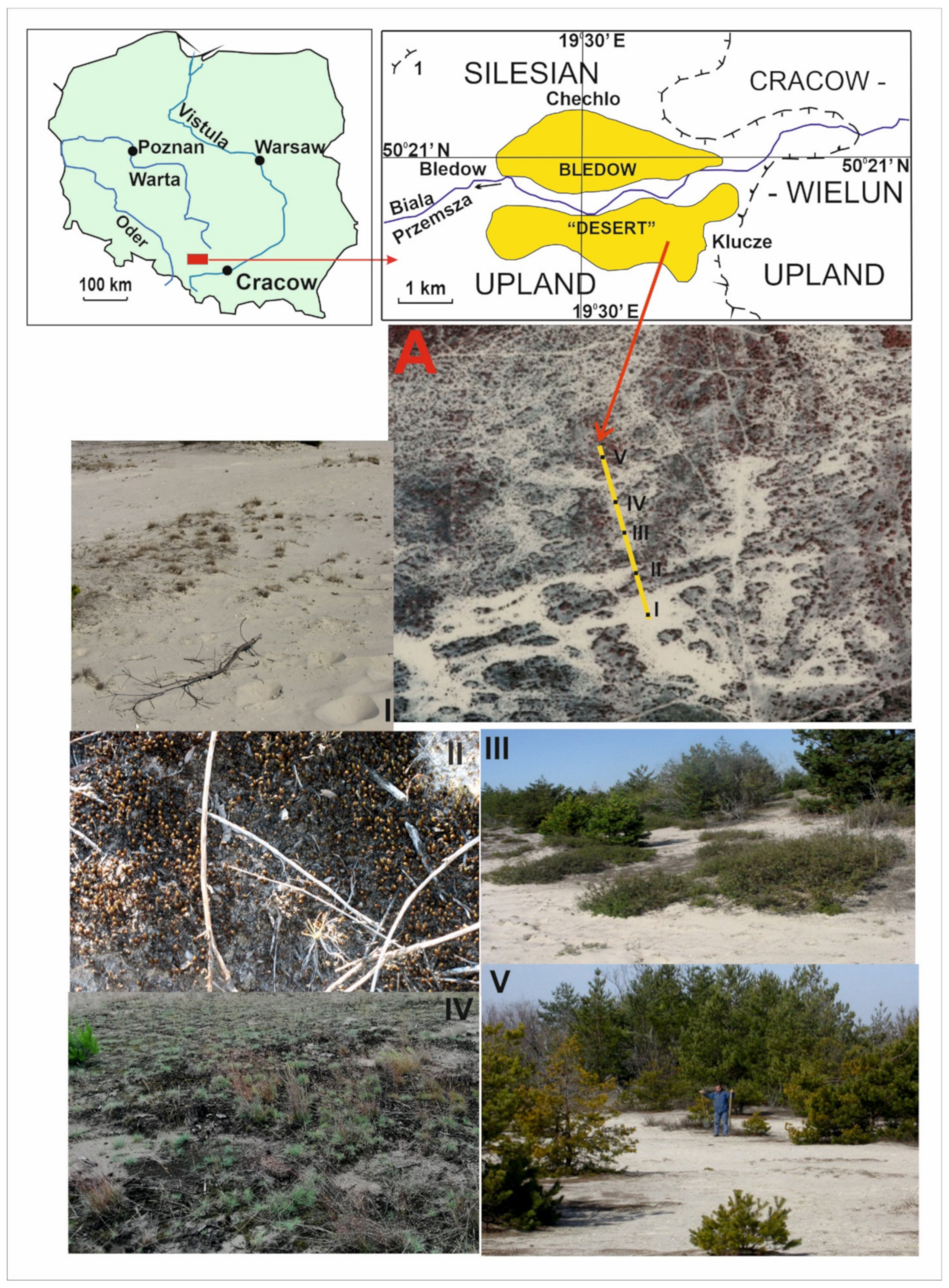
The Błędów Desert is located in the eastern part of the Silesian Upland, in the vicinity of the Upper Jurassic cuesta of the Cracow-Wielun Upland (50°21′17.18″ N 19°30′53.31″ E, Figure 1) in southern Poland between Błędow and Klucze. The origin of this landscape is not natural but is connected to human industrial activities dating from early medieval times, which created a powerful centre for mining and metallurgy [30]. It is known that the ores in this region were exploited for lead in the first half of the 13th century. Charcoal was the basic fuel of the medieval metallurgical industry, but coal was not exploited in Poland until the end of the 18th century. Huge numbers of trees were logged as a result, and this formed an anthropogenic desert in Central Europe [30,48]. From the beginning of the Holocene, the area of the Błędów Desert was covered by a dense mixed forest, which, probably as early as the subboreal period (5100 BP), was dominated by pine trees [62]. The Błędów Desert existed in this form until the beginning of the Middle Ages when, due to the development of lead and silver ore mining, the metallurgical industry, and the usage of forests as a source of fuel for primitive iron works, the forest was completely destroyed, uncovering a sandy bed. Deforestation and degradation of the soil cover in the Middle Ages resulted in damage to the local flora and fauna; hence, naturalists consider the area to be the result of a medieval ecological catastrophe. In this area, vegetation succession, within which the research was carried out, is currently in progress. For details of this, see Rahmonov and Oles [30].
The accumulation, 60–70 m thick, of sand gravel sediments is related to the Pleistocene, mainly—as results from the latest investigations [30,63]—the period of the Odranian (Riss) and Vistulian (Würm) glaciations. The material is mostly of riverine–extraglacial or riverine–prolluvial origin. The area of the Cracow-Wielun Upland, where the material was accumulated as fluvioglacial during the Sanian glaciation (Mindel), was its source, from which it was transported by rivers, filling the system of pre-Quaternary deep valleys [63].
Błędów is situated at an altitude between 301 to 322 m above sea level, and Klucze is located between 347 to 373 m above sea level [64]. Both cities experience significant rainfall throughout the year, even in the driest months. Precipitation is lowest in February, with an average level of 33 mm [65]. The most rainfall occurs in July, with an average of 97 mm. The average annual rainfall is 709–720 mm. The average temperature is 8.6 °C. July is the warmest month of the year (16.5 °C), while January has the lowest average temperature (−3.5 °C). The analysed areas are located close to each other; hence, there are slight differences between them. Both places are located in the zone of moderate, transition climates between maritime and continental zones. West and south-west winds prevail in the study area.
Plot Design
The analysis of the process of phytomass formation and soil development was carried out in five research plots on fresh (naked) sandy surfaces formed as a result of aeolian processes. The five plots were selected based on the fact that they represent all the habitat and soil types present in the study area. The square nature and uniform size of the plots made it easier to calculate the biomass (per unit area). The main criteria used to select the plots was the degree of sand stabilisation (Table 1). They represent different stages of vegetation succession, from primary active deflation fields to the final sod-covered habitats and initial pine coniferous forest. For more information concerning phases and stages of succession, see [30].
The plots were delimited using geodetic methods. Each plot was 400 m2. Pegs were hammered in on each side at distances of 2 m. Pegs on opposite sides were connected by lines to form a net. In this way, 100 squares, each with sides of 2 m, were distinguished within each plot. Additionally, a 1 × 1 m square grid was placed on the surface (2 × 2 m). Detailed plant mapping of plant communities was carried out within this prepared quadrant using a scale of 1:100, which is necessary to identify the participation of plants in terms of area within specific phytocenoses.
2.2. Determination of Phytomass
For the dominant individual species on each plot, an assessment of the aboveground phytomass (a mass of living and dead material that preserves the anatomical structure of the plants) was carried out within an area of 1 m2 with 3 repetitions (the tables show the average result from 3 samples for each analysed organ). Subsequently, the results for the entire area colonised by a given species were recalculated. The aboveground phytomass was recorded when the vegetation of the psammophilous communities was at its maximum, i.e., at the end of August.
In the case of grasses (Corynephorus canescens, Koeleria glauca), the entire aboveground part was treated as one sample, whereas in the case of shrub species (Salix arenaria, S. acutifolia) and trees (Pinus sylvestris), plant organs were divided into leaves, needles, live/dead branches and annual increment. The annual growth of the branches, shrubs and tree was determined in a macroscopic way based on the counting of whorls.
The biomass of aboveground shrubs and trees was determined according to the model tree based on the work of Bazilevič et al. [34]. A model tree is a typical sample tree for a particular category of trees, which is widely used to make a comprehensive assessment of indicators in forest stands (e.g., stock, growth). Model tree analysis was carried out in Plot V and concerned only Pinus sylvestris; 2–3 model trees were selected from the steps close to the average diameter. Trees with a medium shape and crown size for the steps were chosen.
The calculation of belowground phytomass was also carried out within an area of 1 m2 [66], with 3 repetitions. The sampling depths were 0–10 and 10–20 cm. Belowground plant organs were separated from the soil using a sieve with a hole diameter of 0.5 mm, and the roots were divided by diameter: 1–10 or >10 mm (separated visually). In addition, the root mass was washed clean of soil. The roots were not divided into living and dead; they were analysed as one. All the samples of plant material were weighed using a PA64 Pioneer balance and dried in an ES-4610 drying oven at 105 °C to a constant weight, followed by a calculation of the phytomass.
2.3. Soil Investigation
In individual research plots beneath each dominant species, a soil profile was made for a comparison with the plant–soil relationship at the initial stage of soil development. The soil was collected from under the following species: Algal crust and Corynephorus canescens (Plot I), Polytrichum piliferum (Plot II) Koeleria glauca (Plot IV), Salix arenaria (Plot III), S. acutifolia (Plot III) and Pinus sylvestris (Plot V). The ages of S. acutifolia, S. arenaria and Pinus sylvestris were determined by Pressler drill. In total, 21 soil profiles were made (3 of each dominant species on the plot), and samples were taken from each distinguished soil horizon; 81 samples were collected for laboratory analysis. Tables were prepared, showing the average values from 3 samples for each horizon.
The soil samples were submitted for standard physical and chemical analyses, which include particle size distribution using the sieve analysis method (with particle size classes in accordance with the World Reference Base for Soil Resources ([67]); pH in water and in 1 M KCl; hydrolithic acidity (Hh) in accordance with the Kappen method; organic carbon (Corg) in accordance with the Tyurin method; total nitrogen (Nt) in accordance with the Kjeldahl method; available phosphorus (Pavail) in accordance with the Egner-Riehm method [68]. The soil colour was determined according to the Munsell Soil Color Charts [69].
The overall contents of some major elements beneath vegetation communities at mineral horizons were analysed in order to determine the richness of sandy substrates as nutrient sources for plants. Concentrations of selected elements (Ca, Mg, K, Na, P, Fe, Al, Zn) in the soils were measured using ICP-OES (inductively coupled plasma-optical emission spectrometry) following aqueous mineralisation in a solution of nitric and hydrochloric acids (3HCl + HNO3). The analyses were conducted by Bureau Veritas AcmeLabs, Vancouver, Canada.
2.4. Statistical Analysis
Principal component analysis (PCA) was used for statistical analysis of the obtained data. PCA determines the components that constitute a linear combination of the examined variables. Precise PCA enables an indication of the initial variables, which exert a strong impact on the character of the principal components. A correlation matrix, based on the standardisation of the values of the variables [70], was used as a starting point for the analysis. Due to the low level of variance of the values obtained, the selection of principal components was supplemented with the Cattell method (scree plot analysis) [71]. The analysis was performed using PAST 3.
3. Results
3.1. Vegetation Differentiation on the Plots
Calculations of the above- and belowground phytomass beneath the dominant species in the five study plots were performed. This data is presented in Table 2.
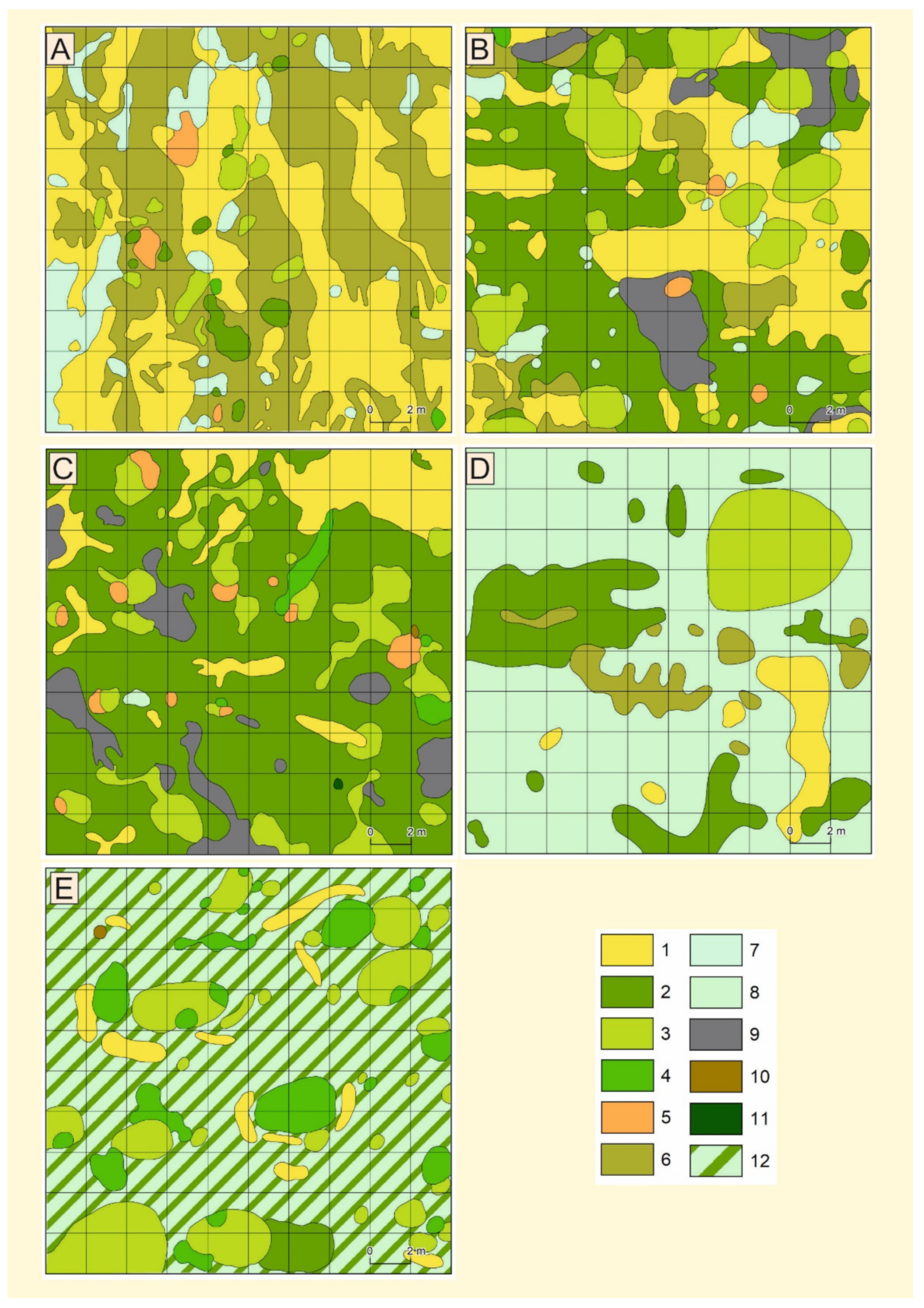
Figure 2 shows the area covered by the distinguished species. Species occur singly in the form of small patches where other species are rare.
3.1.1. Plot I
Detailed mapping showed (Figure 2A, Table 2) that algal communities (Figure 3) dominated this site (48.15%) and were confined to somewhat lower elements of the nanorelief, which receive additional moisture due to the influx of rainwater. The latter confirmed the presence of accumulations of crushed, partially humified plant residues (detritus) on the nanoslopes, characterised by an elongated shape along the slopes. A large portion of the surface was occupied by areas of sands (36.05%) not fixed by vegetation, which were usually close to microelevations. In windy weather, these sands are subject to deflation/waving processes.
Calculations of above- and belowground plant masses carried out in each of the identified communities showed (Table 3) that more than half (56.9%, i.e., 8.55 kg) were formed by sandy willow.
These were dominated by branches with an average age of 6–8 years. In the composition of the underground organs of sandy willow, roots with a thickness of 1–10 mm prevailed (3.06 kg in the community). Apparently, these roots, along with smaller ones (<1 mm), perform active functions in plant nutrition (assimilating roots). The proportion of large conducting roots (>10 mm) was significantly lower due to the youth of the willow in this plot.
In the biomass of the C. canescens community, belowground organs significantly predominated over aboveground ones (more than tenfold; Table 3). Their mass extended in the soil to depths of 12–15 cm, where the sandy mass of the horizon was densely intertwined. The phytomass of P. piliferum was 0.65 kg for the whole community; its biomass was 7.2 times smaller than C. canescens (Table 3). S. acutifolia (0.10 kg) and P. sylvestris (0.019 kg) were not of great importance at this stage in the formation of biomass.
3.1.2. Plot II
Here, unlike in Plot I, the area of moving sands and algal communities was significantly reduced, the areas of green moss willow and pine communities were expanded, and the pines were larger and in better condition. The accumulation of organic matter was also increased (Figure 2B). Sandy areas rich in organic matter were actively colonised by K. glauca (0.18 kg), which systematically replaced C. canescens (0.08 kg; Table 4).
The calculations of plant biomass therein showed them to be 13.73 times greater than in the green moss–algae phytocoenosis (Table 3 and Table 4). The greater part of this was formed by sandy willow, which was 33.72 kg in the aboveground phytomass and 155.46 kg in the belowground phytomass. At the same time, attention was drawn to the less distinct excess of reserves in belowground organs than in aboveground organs (Table 4). In the latter, the main mass was also formed by roots of medium diameter (1–10 mm), most of which served as feeding roots.
As in the phytocenosis (Plot I), S. acutifolia was represented here by dead individuals. The biomass of the sand grass community had increased here as a result of the expansion of the K. glauca and green moss communities.
3.1.3. Plot III
Detailed mapping showed (Figure 2, Table 2) a further reduction of bar sands not fixed by vegetation, and K. glauca communities represented an expansion of the area occupied by downtrodden mosses (mainly P. piliferum) and areas with an accumulation of crushed organic matter (plant detritus). The growth of Scots pine, its good condition, and its formation of separate clumps were remarkable, as was the appearance of individual trees of juniper and birch.
The greatest volume of phytomass was represented by S. arenaria (86.51 kg; Table 5), which was 1.75 times more than P. sylvestris. In total, there were 4 individual pines with an average age of 9 years, an average trunk length of 178 cm, and diameters of 7 cm at the base and 2 cm at chest height. The main part of its biomass (22.22 kg, i.e., 45% of the total aboveground biomass) consisted of the trunk. The average tree possessed 17 branches, ranging in length from 26 to 52 cm (in the model branch, 37.9 cm). Their reserves ranked second (trunk) in aboveground pine biomass (15.96 kg, i.e., 32.45%). They were characterised by a high growth rate and a high level of fecundity and vigour. The latter quality, as well as the absence of needle necrosis, obviously indicates favourable conditions for the growth of the plant.
3.1.4. Plot IV
Further reduction in bare sands (4.79% of the total area; Table 2 and Table 6), areal dominance of the K. glauca community (65.67%), and local distribution of green moss and algal communities (15.95% and 5.18%, respectively; Table 2) were observed here. In this phytocenosis, 8.4% of the total area was occupied by Salix arenaria clumps confined to a wide aeolian hillock. Festuca ovina, Arabis arenosa, Leontodon hispidus, Elymus arenarius, and some lichens from the genera Cetraria, Cladonia, and Cladina were also present.
In terms of plant mass reserves, the phytocenosis under consideration is almost five times richer than the green moss–algae. The main part of its aboveground phytomass (64.5%) was formed by a K. glauca community (Table 6), in which an area of 1 m2 accumulated 3 times more aboveground biomass in comparison with a similar community in the sand grass–willow–green moss phytocenosis, and, in terms of underground biomass, 1.9 times less (compare Table 4 and Table 5).
The second-largest percentage of the total plant mass was taken up by the sand willow community. In terms of an area of 1 m2, this mass was almost 7 times less than its equivalent in the pine–willow–moss phytocenosis (see Table 5). This was associated with the younger age of the curtain and, consequently, lesser growth of branches and of sandy willow roots. The P. piliferum community made up the smallest amount of the biomass reserves, both when recalculated per 1 m2 and for the community as a whole.
3.1.5. Plot V
Further diminution was noted in the area of nonfixed sands (4.79% of the total area) and the P. piliferum community (1.79%; Table 2); the area occupied by Scots pine and willow communities expanded significantly (Figure 2). The spaces between willow and pine clumps were occupied by clumps of K. glauca, between which grew P. piliferum.
Calculations of the total phytomass in this phytocenosis showed (Table 7) its highest reserves in comparison with the phytocenoses considered above (Table 3, Table 4, Table 5 and Table 6). These reserves are 26 times higher than the green moss–algal phytocenosis (Plot I), 1.93 times higher than the sand grassland–willow phytocenosis (Plot II) and 6.17 times higher than the sand grassland–willow–green moss phytocenosis (Plot IV). The counts showed that the main part (more than 90%) of the phytomass was formed by S. arenaria.
In this plot, the phytomass of aboveground organs was significantly (3.1 times) greater than the mass of underground organs and was formed mainly by branches, both living and dead (dry), in S. arenaria. Obviously, this indicated unfavourable growing conditions for this species and the potential for its displacement by other plants, such as Scots pines, which regenerate well under a willow canopy.
The Scots pine community ranked second in its participation in the formation of the biomass of the considered phytocenosis. In this case, the prevalence of the aboveground phytomass was also observed (Table 7).
Most of this phytomass was formed by stem wood (62%, i.e., 45.09 kg in the community) and branches (18.8%, i.e., 13.71 kg in the community). In terms of plant mass, the communities of P. piliferum and K. glauca were generally close to their equivalents in the phytocenoses discussed above.
3.2. Soil Morphology
The results of the analysis show no major differences between study plots in terms of grain size. The analysed soil material was dominated by grains of the fraction 0.5–0.25 mm (medium-grained sand, 57% on average), followed by the 0.25–0.1 mm (fine sand, 22.8% on average), 1.0–0.5 mm (coarse sand, 18% on average) and <0.1 mm (very fine and silt dust fraction and floatable parts, 2.5% on average) fractions. The last-mentioned fraction was most abundant in the organic-humus (OA) and humus (A) horizons (Table 8).
The formation of soil under individual plant communities in all tested plots (Plots I–V) showed morphological differentiation into organic (O) and humus (A) horizons. The organic horizon (O) was differentiated into Ol, Of, and Oh subhorizons (Table 9) only under S. acutifolia (Plot IV) and P. sylvestris (Plot V), forming a general profile structure of the type Ol-Of/hAB(fe)-BC-C and Ol-Of-Oh-A-AC-C. The thickest organic and humus horizons occurred directly in the middle of the canopies of trees and bushes. The soils were defined as Leptosols and Distric Arenosols.
3.3. Chemical Properties of the Soils in the Plots
The analysed soil was acidic and slightly acidic in terms of its reaction (pH). A very acidic reaction was found in the organic subhorizons under the canopy of P. sylvestris, characterised as follows: Ol: 3.9 in H2O and 3.2 in KCl; Of: 4.3 in H2O and 3.4 in KCl; Oh: 4.3 in H2O and 3.4 in KCl. The horizons under S. arenaria (pH—Ol/f/h: 5.6 in H2O, 4.9 in KCl) and S. acutifolia (pH—Ol: 5.5 in H2O, 5.1 in KCl; Of: 5.8 in H2O and 5.2 in KCl) were acidic or weakly acidic (Table 9). The situation was similar in the case of hydrolytic acidity resulting from the decomposition of pine litterfall. This represents a clear modification of habitat under the influence of a specific plant species (with xeromorphic morphology, high albedo ability, low nutrient requirements) resulting from the chemical composition of its litterfall in the form of a lack or low concentration of ash elements (among others).
The maximum contents of organic carbon (Corg) and total nitrogen (Nt) were found in almost all organic-humus horizons (OA, under Algae, Corg, 1.10, Nt, 0.060%; P. piliferum community, Corg, 8.49%, Nt, 0.292%) and organic horizon with its subhorizons (under S. arenaria, O (Ol/f/h): Corg, 12.30%, Nt, 0.492%; S. acutifolia, Ol: Corg, 49.20%, Nt, 1.560%; Of/h: Corg, 11.50%, Nt, 0.558%; P. sylvestris, Ol: Corg, 49.40%, Nt, 0.903%; Of: Corg, 32.12%, Nt, 0.615%; Oh: Corg, 19.51%, Nt, 0.508%). The range of the C/N ratio is relatively narrow, with averages of 25 in organic and humus horizons for S. acutifolia and S. arenaria (Table 9). On the other hand, under P. sylvestris, this index is characterised by a wide range, from 38 to 54, indicating poor decomposition of organic matter.
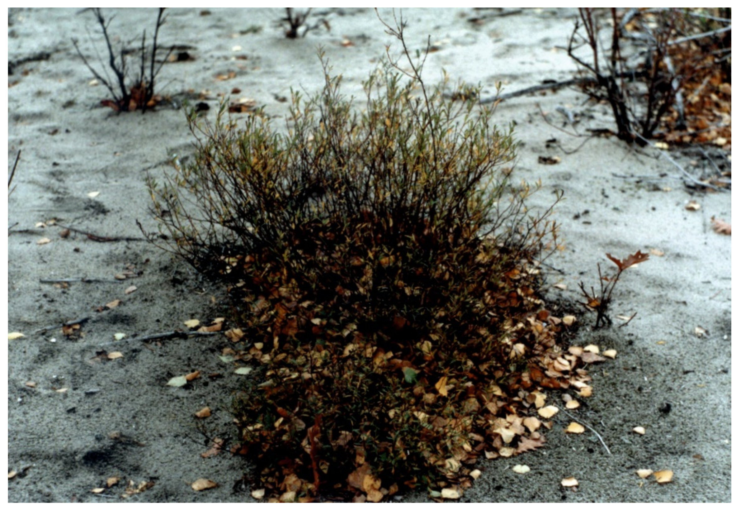
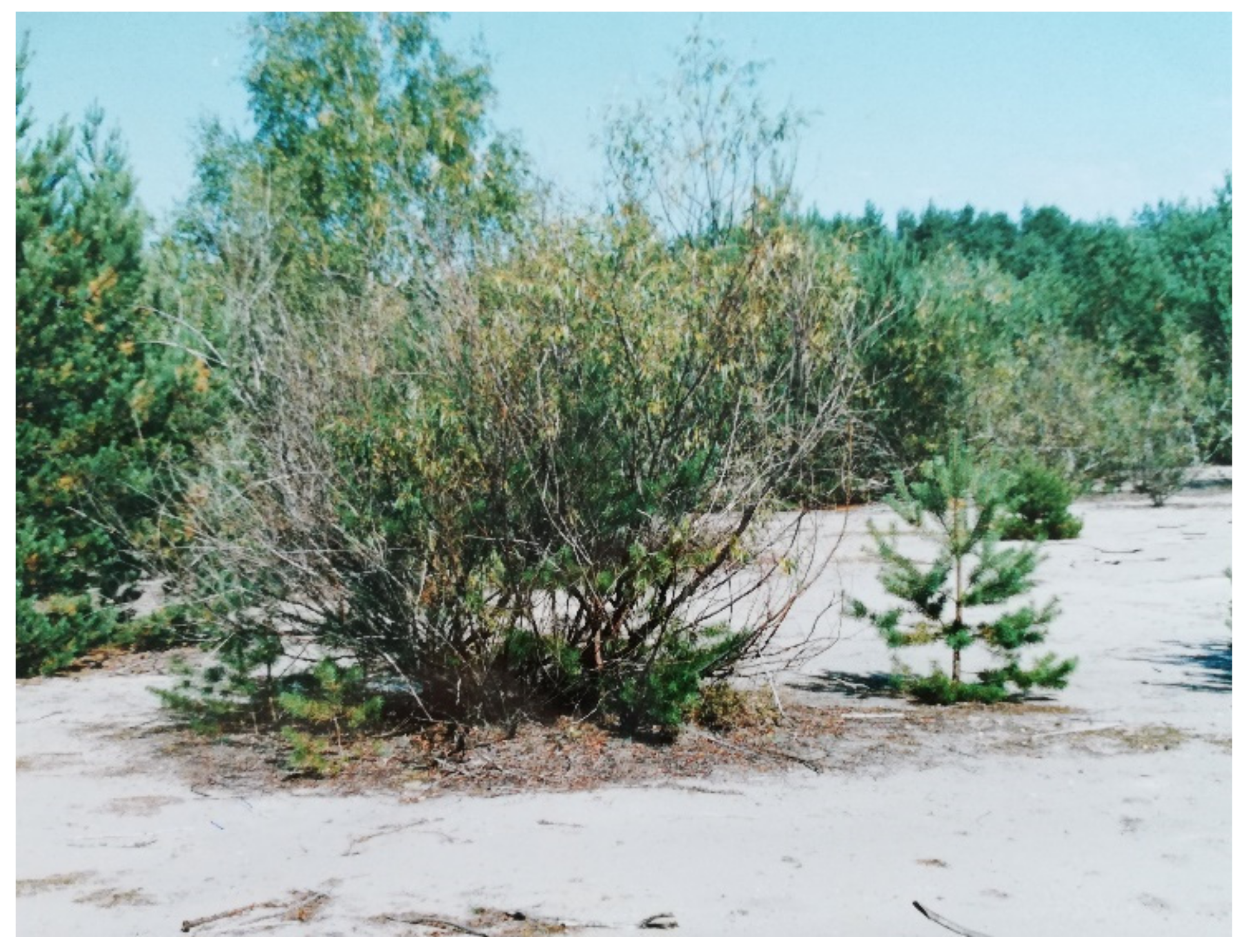
The content of organic carbon (Corg) in individual plots under the dominant species in the humus (humus) horizon ranged from 0.28% to 1.42%. Its maximum concentration (Corg, 1.42%) was found in a clump of S. arenaria, which, apart from its own litterfall (plant litter), also retained other organic debris transported downwind, thanks to its specific structure and the shape of the clump, which also functioned as a trap (Figure 4).
Significant organic carbon content was also noted in the OA horizon (under the algae and P. piliferum community; Table 8). Algae adhered to the surface of sand grains and often formed woolly mats constituting the first source of organic matter on the surface of bare quartz sand. As a result, a notable share of total nitrogen was found in the initial humic horizons (often <1 mm), ranging from 0.015 to 0.072, whereas in the parent rock (without traces of algae), nitrogen was present in very small amounts, with a maximum content of only 0.013%.
Available phosphorus (Pavail), as a deficit element for plant development in extremely poor sandy habitats of the studied area, plays an important environmental role. Its maximum contents were found in organic and organic-humus horizons, where they ranged from 10.41 to 65.23 mg/kg. Notable participation of Pavail was also observed in the soil mineral horizons under K. glauca (24.10 mg/kg) and S. acutifola (25.11 mg/kg). It did not differ significantly in the remaining horizons (Table 9).
3.4. Differentiation of Phytomass in the Plots
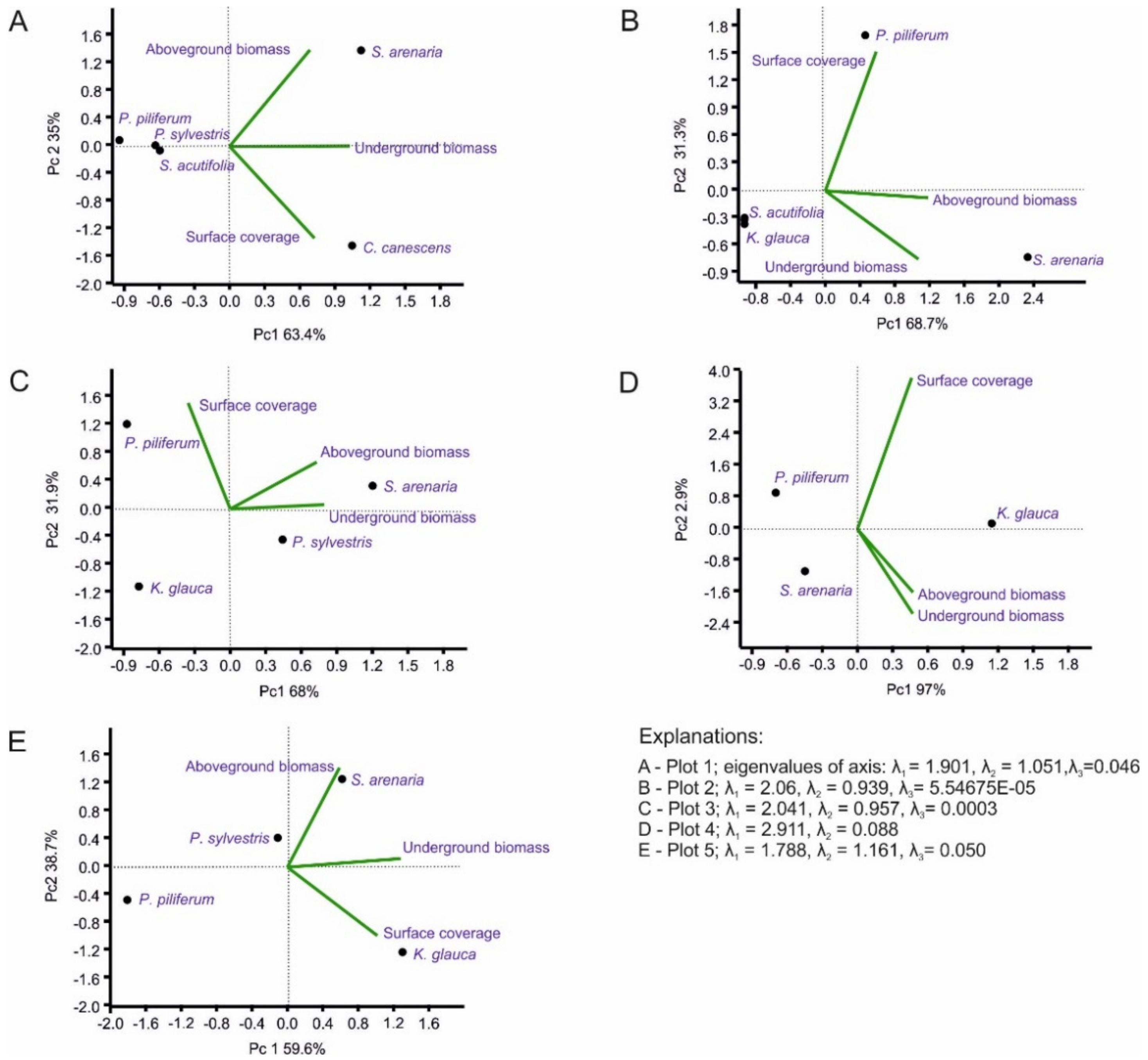
In order to present the relationship between phytomass production in the plots, principal component analysis (PCA) was conducted (Figure 5). The analysis included particular dominant plant species concerning above- and belowground biomass. The PCA results enabled the determination of general patterns of correlation between the major variables. As dependent variables, the volume by weight of biomass and the share in the surface coverage of the dominant species were used. The obtained configuration of three variable outputs for each plot can be described using only one combination.
The first component (PC1) of each plot shows a variance in the range of 60% to 97%. PC2 and PC3 may be omitted due to the low degree of explanation of the total variation (low variance). In the case of Plot IV, PC1 is quite significant, explaining 97% of the variation (Figure 5D).
The values of the variables of this principal component were characterised by a high degree of correlation (r = 0.99). Thus, the first axis captured the ratio between above- and belowground biomass. Vegetation with high scores on this axis was characterised by a significant share in the production of biomass at this stage of succession. PC2 was interpreted as the relationship of the axes of the belowground biomass/surface coverage of dominant species. The variables for Plots II (r = 0.92) and III (r = 0.93) also showed a high correlation coefficient with lower variance (Figure 3B). In this case, PC1 is also interpreted as the relationship between above- and belowground biomass and the second axis as the relationship between the belowground biomass and surface coverage of the dominant species ratio. Other plots showed lower levels of variation: Plot I, 63%; Plot V, 60%.
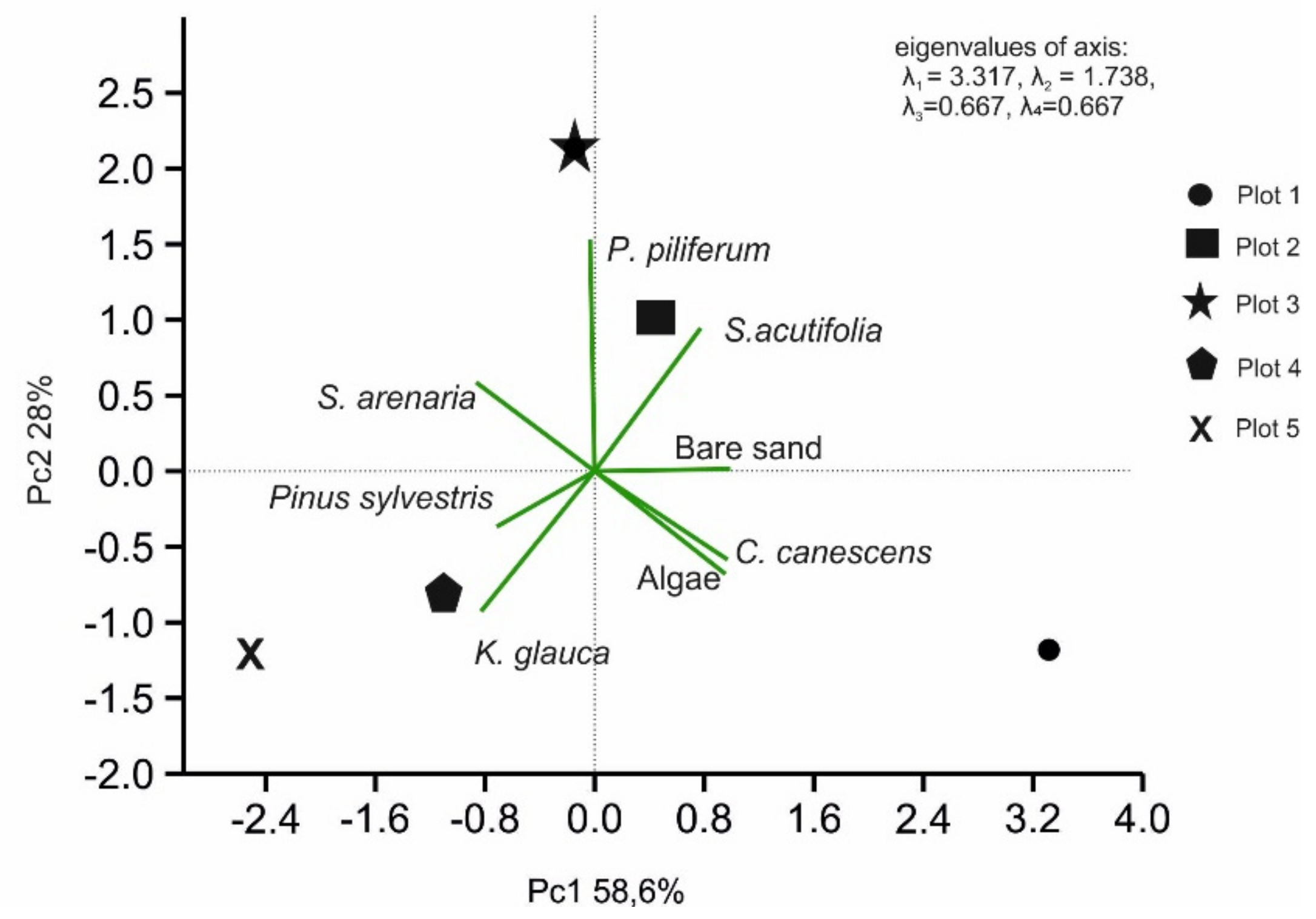
Moreover, using PCA analysis, we studied the compound dependence of land cover through dominant plants and the occurrence of sandy soil for the five-plot study. In this case, the pattern of four variable outputs can also be described using one combination of PC1, the variance of which is 58.6% (Figure 6). Based on the scree plot, PC2 can be used for dependence analysis (28% value of variance). PC1 is defined as the ratio of the participating species C. canescens and algae for individual plots. The PC1 variables showed a strong correlation (r = 0.99). The second axis was interpreted as the relationship between C. canescens and sandy surfaces (r = 0.86).
3.5. Contents of Selected Macroelements
Information about the total chemical composition of the soil is very important from the point of view of both soil-forming processes and the contents of potential nutrients for plants, which determine their rate of development and growth in extreme habitats. Analyses of the contents of the main elements, such as Ca, Mg, K, P, Fe, Al, and Zn, showed little differentiation; slightly higher contents in some cases (Table 10) were observed in humic (A) and organic-humic (OA) horizons, resulting from the presence of soil organic matter. Among the examined elements, Al dominates in all plots, with its content in the parent rock ranging from 8800 to 14,800 mg/kg.
The rank of concentrations of macroelement metals in the organic-humus (OA), humus (A), mixed (AC), and parent rock horizons is given below:
- Algal crust-OA: K > Na > Al > Mg > Ca > Fe > P > Zn
- Corynephorus canescens-A: Al > Fe > Na > Ca > P > K > Mg > Zn
- Corynephorus canescens-C: Al > Fe > Na > Ca > K > Mg > P > Zn
- Koeleria glauca-A: Al > Fe > K > Na > Ca > Mg > P > Zn
- Salix arenaria-A: Al > Fe > K > Na > Ca > P > Mg > Zn
- Salix acutifolia-A: Al > Fe > K > Ca > Na > Mg > Zn > P
- Pinus sylvestris-A: Al > K > Ca > Na > Zn > Fe > Mg > P
- Pinus sylvestris-AC: Al > K > Fe > Na > Ca > Mg > Zn > P
4. Discussion
The below- to aboveground biomass ratio is a variable reflecting a plant’s response and adaptation strategies in the face of environmental stress as well as an important parameter for the terrestrial carbon cycle [35,72,73]. Such processes are initiated in harsh habitats by microorganisms invisible to the naked eye. The apparent pioneering stage involves communities formed by bacterial and fungal microflora. However, the microflora of soils in the Błędów Desert has not yet been studied. Therefore, we can only assume that, at this stage, the main part of soil formation under these communities consists of an accumulation of organic matter. In fact, soil profiles are absent under pioneer succession, but conditions are conducive to the encroachment of organisms with a high level of ecological requirements [52,74,75]. These organisms are algal communities (Figure 3). They actively develop in spring and early summer, but as early as June, they die off and quickly decompose, resulting in humus enrichment of the superficial thin crust of sands, its noticeable compaction, and weak cementation [48,49,50]. The algal crust, extremely rich in sugars, nitrogen, and sulphur, contains organic compounds [52,53]. Such surfaces are inhabited by green mosses (Polytrichum), which form a significantly larger biomass (Plot I). Their rhizoids penetrate deeper than algae, envelop and hold the grains of sand, limit their swelling, and inhibit or retard aeolian processes.
In the plots analysed, apart from the dominant species (for which the calculation of phytomass was performed), there were taxa of both early (Cerastium semidecandrum, Cardaminopsis arenosa, Elymus arenarius, Scleranthus annuus, S. perennis, Jasione montana, Festuca ovina, Herniaria glabra) and late (Betula pendula, Quercus robur, Juniperus communis) successional species, adapted to development in sandy habitats, which usually occur singly and play no significant role in the formation of phytomass. Woody species indicated the further direction of succession [30]; for example, specimens of P. sylvestris were found in Plot I.
C. canescens initiates the first stage of succession, colonising bare and nutrient-poor sands (often shifting) in which it is often buried. It tolerates this process well and develops better thanks to vertical growth and adventitious root development. Ecological studies have confirmed that it also causes the high soil aeration preferred by this species [76,77,78]. Thus, phytomass, especially belowground, grows systematically; its soil-forming role at this stage is also associated with the stabilisation of moving sand and the facilitation of encroachment of other early successional species such as K. glauca.
Root mass plays an important role in increasing the amount of organic matter in the soil, especially in areas with extreme environmental conditions (dry, poor, high temperatures) [79,80]. K. glauca, in contrast to C. canescens, is characterised by a hard, thick, and long root system, often reaching 2 m deep, which decomposes enriched sandy soil with nutrients at various depths [78]. Within the dunes, the direction of root development follows the humus-rich layers [81]. Phytomass produced by K. glauca is important in the process of changing soil features [27,52,60].
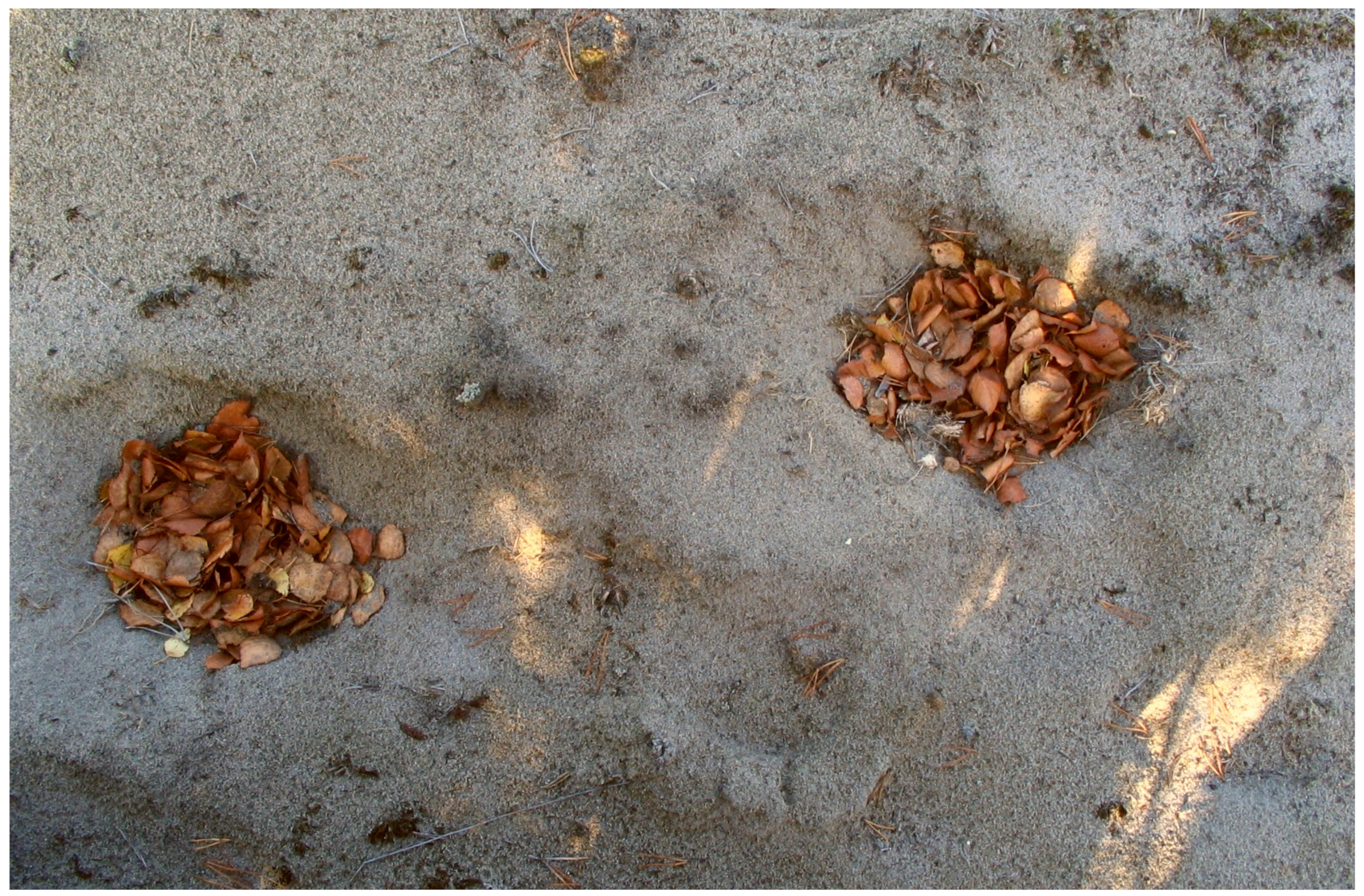
PCA analysis showed a strong correlation (r = 0.99) in underground and aboveground phytomass in Plot IV, dominated by S. arenaria and P. piliferum (Figure 3A,D), in contrast to Plot I. This has an impact on the development of soils on these plots (Table 9). A strong correlation was observed in the algal community and C. canescens as an early succession species in Plot I (Figure 4). These phenomena have been confirmed by many authors [24,25,27,29,30]. Autochtotonous or allochthonous organic matter, transported by the wind from neighbouring areas, does not always accumulate stably around grass clumps and under the canopy of shrubs and trees and is often subject to further transport. In micro- and macrodepressions of the terrain (i.e., traces of shoes and tyres; Figure 7) as well as organic debris devoid of vegetation on the surface (mainly leaves and small twigs), they are often covered with sand and, in decomposing, increase humidity and the presence of nutrients such as C, N, P, and Mg [60,81].
Subsequently, such areas are colonised by other species, with an irregular distribution of vegetation, referring to the shape and nature of the traces. The content of minerals in the initial stage of succession is closely related to the increasing biomass. All of this indicates that increasing the biomass favours the accumulation of organic matter, which is the basic substrate for the formation of the humus horizon and, consequently, the entire soil profile. Similar processes have been found on dune and inland sands by many researchers [29,52,82,83].
The process of biomass formation is closely related to the strategy of plants adapting to extreme habitats in terms of low concentrations of nutrients. S. acutiofolia and S. arenaria are properly adapted to the conditions of intensified aeolian processes, both in terms of morphology and ecophysiology [84]. As a result, they develop well and produce much more biomass each year than other species. The process of biomass formation also favours the encroachment of other late successional species [25,27,85]. The produced biomass is often covered with a fresh layer of sand (which either penetrates the soil or remains on its surface), enriching the soil with organic substances (Figure 7). This is one of the most important forms of habitat formation by plants, as dead remains and falling leaves accumulate in the soil and on its surface, providing saprophytes with essential food. In turn, the activity of saprophytes influences the edaphic conditions of plant growth, e.g., humidity ratios, the content of mineral nutrients, soil aeration, pH, and other paedogenetic changes in the soil. Thus, increasing the biomass entails the acceleration of not only soil processes but also other ecosystem processes [86].
Soil Formation Processes and Features in the Plots
The analysed soils are characterised by a sandy granulometric composition, rich in quartz but low in nutrients. The soils are characterised by weak absorption capacity, a high level of air and water permeability, and little cohesion. These properties are inherited by soils formed on sands, manifested in the predominance of oxidative processes in their profile, low rates of dispersion of relatively large particles into smaller ones, the presence of a leaching type of water regime, and compliance with deflationary processes. Their fine earth is clearly dominated by sand fractions and especially by particles of medium sand (1.00–0.25 mm). The distribution of the content of all fractions is weakly differentiated due mainly to the varying timing of the aeolian influx. The insignificant enrichment in the silt of the upper, most humified, warmed epipedon (surface horizon) is obviously caused by slightly increased weathering activity in comparison with deeper horizons. At deeper levels, the humus content decreases sharply, which correlates with very low root reserves. Roots are characterised by high ash content, as a result of which the bases, mobilised following the decomposition of root masses, almost completely neutralise the newly-formed humic acids.
The direction of soil-forming processes under the algae associations P. piliferum, C. canescens and K. glauca do not differ principally from each other. However, the forming of the humus horizon beneath them is conditioned by the amount of biomass (Table 3, Table 4 and Table 5).
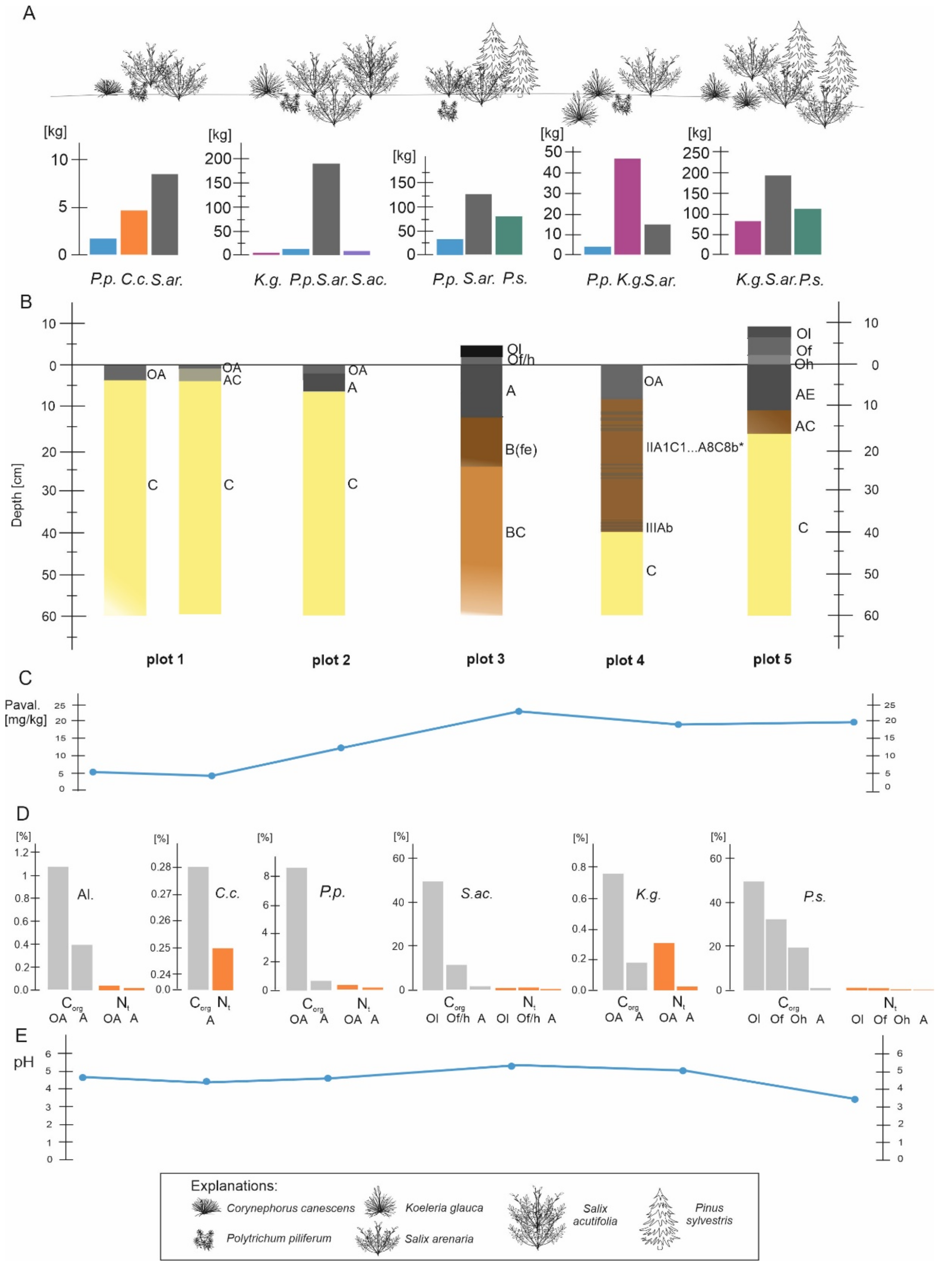
Figure 8 shows the variability of biomass, which determines the formation of soil horizons, mostly organic (Ol, f, h) and organic-humus (OA). This effect was found under P. sylvestris, which determines the soil reaction’s nature (very acidic) under its canopy. Higher values of Corg, Nt, and phosphorus, available in individual profiles, are also related to the degree of organic horizon development (Figure 8) and its decomposition. Despite the weak development of OA horizon under algocenoses, the humus content in the A horizon is higher than under Corynephorus canescens and Koeleria glauca. It is associated with the fact that algae thallus will entirely decompose annually and form an epihumus horizon [51,52,53] compared to vascular species [86,87].
The main source of organic matter necessary for the formation of the humus horizon at the initial stages under algae, bryophytes, and grasses is their organs (above- and belowground). After death, the stems and roots quickly decompose and are transformed into humus (by bacterial microflora), contributing to the accumulation of humus and the initiation of a thin humus horizon. This is also facilitated by the high ash content of various organs of C. canescens and K. glauca [58], as a result of which the organic acids formed (during decomposition and humification) immediately interact with bases mobilised during the mineralisation of root litter and are neutralised and transferred from mobile forms into immobile or low-mobility forms. Consequently, they accumulate in situ and form a humus-accumulative horizon (OA) in the soil (Table 8). P. piliferum communities at the analysed sites grow on soil “prepared” by the algal community. The assimilated parts of species are covered by a heavy accumulation of deflating sand. Their rhizoids, immersed in sand to a depth of 1–3 cm, hold the sand together. Between the stems, the bryophyte retains the litter of various plants transported by the wind, which, in turn, also favours the accumulation of organic matter and, consequently, the formation of the OA horizon. The plant mass reserves of the P. piliferum community are significantly (7.3 times) greater than those of the small-grained community, but their effect on soil formation is much less.
As opposed to grassland communities, a distinct difference in soil formation is observed under S. acutifolia and P. sylvestris. The soil cover under the willow and pine trees appear in the form of patches and are related to the shape and size of their canopy (Figure 9).
Soil developing under P. sylvestris differs from soil under short-grass vegetation in terms of the following features: the presence of a sufficiently thicker litter of needles, bark, twigs, and dry cones of Scots pine; the presence of a thin podzolised mineral horizon in the form of white quartz grains as a consequence of fulvic acid activity and weak expression of the illuvial horizon. The former feature is due to the predominance of the rate of incoming pine litter over the rate of its decomposition. As is known, coniferous litter [87,88,89] is rich in tannins, waxes and resins, which limit the processes of decomposition by bacterial microflora. Such plant litter is usually decomposed by fungal microflora, which is, however, not very active in this case, as indicated by the practically undisturbed upper part of the litter (Ol) and the weak decomposition of the lower part (Oh). Weak podzolisation and the thinness of the A horizon are obviously due to two factors: a low supply of organic acids migrating from the weakly decomposed organic horizon (Ol/f/h) into the mineral layer, the brief duration of soil formation under the pine canopy (20–26 years), and the periodic supply of fresh aeolian material.
Soils formed under S. acutifolia growing next to P. sylvestris (Table 8) are characterised by a fundamentally different structure and different features, such as a significantly thinner organic horizon and a higher rate of decomposition, especially in the lower part of the horizon; the presence of a relatively thick horizon enriched with humus, with a thicker humus horizon; the absence of morphologically visible podzolisation of the upper part of the mineral strata. Humic acids are practically inert (nonmobile) with respect to primary soil minerals; this is the main reason for the nonpodzolisation of soils [85] under S. acutifolia and S. arenaria.
The noted differences in the soils under a canopy of willow and pine are obviously explained by the fundamentally different biochemical and ash composition of willow litter compared to pine litter. Willow litterfall, like that of other deciduous plants, is rich in ash elements and nitrogen [90]; it differs from pine litter, as it is characterised by significantly lower contents of tannins, waxes, and resins. Therefore, of course, it is decomposed mainly by bacterial microflora, the result of which, in the composition of the newly formed humic acids along with fulvic acids (which are formed mainly during the decomposition of coniferous waste), a great quantity of humic acids are formed. It is known ([87,88,89] that humin acids are poorly soluble in water and therefore inactive, which is facilitated by their averaging by bases mobilised during the decomposition of high-ash litter. Obviously, therefore, newly formed humic acids accumulate directly under the litters, imparting a dark colour to the organic-mineral horizons (OA horizon). A much smaller, nonaveraged portion of these acids migrates over short distances, causing the formation of accumulative horizons A. It should be emphasised that the soil formed under a canopy of willow and direct pines relates to the shape and size of the canopy. This phenomenon has been found in many arid areas around the world [60,91,92,93].
The fundamental differences in soil profiles under the vegetation of sandy grasslands (P. piliferum, Corynephorus canescens, Koeleria glauca) and under S. arenaria, Salix acutifolia and P. sylvestris can be explained by the instability of the soil and the intense influx of fresh aeolian sand. The predominance of sandy fractions in the fine earth of the soil texture of the investigated soils determines its poor alkaline and alkaline earth elements, as well as zinc and oxides of Fe, Al, Mg, Ca, Na, K and P (Table 10). The distribution of their content in the soil profile is poorly differentiated due obviously to the multitemporal influx of aeolian sand and some variation in its mineralogical composition [92]. Multiple redeposition and, therefore, mixing of the aeolian sands most likely caused their homogenisation in chemical composition. Modern soil formation processes were of short duration here; as a result, they had a noticeable effect only on the most mobile elementary soil-forming processes. These include the formation of organoaccumulative horizons (OA) and adjacent surface mineral horizons from below.
5. Conclusions
The degree of stabilisation of the loose sandy substrate determines vegetation colonisation, which affects both the amount of phytomass and the formation of the initial humus horizon. Bare sands are colonised by aboveground soil algae (epipsammism); their role is to fix loose sand and facilitate the encroachment of new species with higher ecological requirements. The dead algae crust forms the thin initial humus layer, creating favourable conditions for new species.
Under the species analysed (P. piliferum, C. canescens, K. glauca, S. arenaria, S. acutifolia and P. sylvestris), changes were found in the amount of phytomass (above- and belowground) and the formation of initial soil horizons.
During the primary succession of the thalli of algae, bryophytes and the remains of dead C. canescens, K. glauca is a source of organic matter necessary as a nutrient and base material for initiating soil formation processes.
In psammophilous grasses, C. canescens and K. glauca, fixing loose sand and its dead tissues in the initial stages of succession, are the source of soil organic matter. In these species, belowground phytomass dominates over aboveground phytomass. A different and significant effect, compared to the other analysed species, was found under a canopy of S. acutifolia and S. arenaria, with a significant impact on soil-forming processes. Soft willow leaves (plant litter) quickly decompose, leading to the relatively rapid formation of the humus horizon, in contrast to weakly decomposing pine litterfall, which is clearly visible in the thickness of the organic horizon.
The soils under canopies of willow and pine form in patches, directly related to the shape and size of their canopies. A clear relationship was found between the changing amount of phytomass and the morphology of soil profile structure and physical (pH) and chemical (Corg, Nt, Pt and Pavail) properties of the soil.
Complementary studies comparing changes in phytomass and soil characteristics confirmed the close relationship between vegetation development and the initial soil (Arenosols) in sand substrates. This finding is much more reliable than a mere list of species at various stages of succession. The biogeochemical processes and changes occurring in the initial ecological systems, which are the initial stages of succession, are of great importance.
Author Contributions
Conceptualization, O.R.; methodology, O.R., M.R., and S.S.; software, M.R.; validation, O.R., M.R, and S.S.; formal analysis, O.R.; investigation, O.R.; resources, O.R.; data curation, O.R.; writing—original draft preparation, O.R., M.R., and S.S.; writing—review and editing, O.R.; visualization, M.R. and S.S.; supervision, O.R.; project administration, O.R. All authors have read and agreed to the published version of the manuscript.
Funding
This research received no external funding.
Institutional Review Board Statement
Not applicable.
Informed Consent Statement
Not applicable.
Data Availability Statement
Not applicable.
Acknowledgments
We gratefully acknowledge anonymous reviewers for their constructive comments.
Conflicts of Interest
The authors declare no conflict of interest.
References
- Titlyanova, A.A.; Bazilevich, N.I.; Shmakova, E.I.; Snytko, V.A.; Dubynina, S.S.; Magomedova, L.N.; Nefedyeva, L.G.; Semenyuk, N.V.; Tishkov, A.A. Biological Productivity of Grasslands. In Geographical Regularities and Ecological Features, 2nd ed.; ISSA SB RAS: Novosibirsk, Russia, 2018; p. 110. [Google Scholar]
- Dickerman, J.A.; Stewart, A.J.; Wentzel, R.G. Estimates of net annual aboveground production: Sensitivity to sampling frequency. Ecology 1986, 67, 650–659. [Google Scholar] [CrossRef]
- Schenk, H.J.; Jackson, R.B. The global biogeography of roots. Ecol. Monogr. 2002, 72, 311–328. [Google Scholar] [CrossRef]
- Bazilevič, N.I.; Titlânova, A.A. Biotičeskij Krugovorot na Pâti Kontinentah: Azot i Zolʹnye Élementy v Prirodnyh Nazemnyh ékosistemah; Izdatel‘stvo SO RAN: Novosibirsk, Russia, 2008; pp. 1–381. [Google Scholar]
- Rodin, L.E.; Smirnov, N.N. Resursy Biosfery (Itogi Sovetskih Issledovanij po Meždunarodnoj Biologičeskoj Programme); Nauka: Sankt Peterburg, Russia, 1975; pp. 1–287. [Google Scholar]
- Kazanceva, T.I. Produktivnost’ Zonal’nyh Rastitel’nyh Soobŝestv Stepej i Pustyn’ Gobijskoj Časti Mongolii; Nauka: Moskva, Russia, 2009; pp. 1–336. [Google Scholar]
- Alaback, P.B. Biomass regression equations for understory plants in coastal Alaska: Effects of species and sampling design on estimates. Northwest Sci. 1986, 60, 90–103. [Google Scholar]
- Cairns, M.A.; Brown, S.; Helmer, E.H.; Baumgardner, G.A. Root biomass allocation in the world’s upland forests. Oecologia 1997, 111, 1–11. [Google Scholar] [CrossRef]
- Chiarucci, A.; Wilson, J.B.; Anderson, B.J.; de Dominicis, V. Cover versus biomass as an estimate of species abundance: Does it make a difference to the conclusions? J. Veg. Sci. 1999, 10, 35–42. [Google Scholar] [CrossRef]
- Schultze, E.D.; Lloyd, J.; Kelliher, F.M.; Wirth, C.; Rebmann, C.; Luehker, B.; Mund, M.; Knohi, A.; Milyukova, I.; Schulze, W.; et al. Productivity of forest in the Euro-Siberian boreal region and their potential to act as a carbon sink—A synthesis. Glob. Chang. Biol. 1999, 5, 703–722. [Google Scholar] [CrossRef]
- Titlyanova, A.A.; Romanova, I.P.; Kosych, N.P.; Mironycheva-Tokareva, N.P. Pattern and processes in above-ground and below-ground components of herbsland ecosystems. J. Veg. Sci. 1999, 10, 307–320. [Google Scholar] [CrossRef]
- Usol’cev, V.A. Fitomassa Lesov Severnoj Evrazii: Baza Dannyh i Geografiâ; UrO RAN: Ekaterinburg, Russia, 2001; pp. 1–708. [Google Scholar]
- Heinrichs, S.; Bernhardt-Römermann, M.; Schmidt, W. The estimation of aboveground biomass and nutrient pools of understory plants in closed Norway spruce forests and on clear cuts. Eur. J. Forest Res. 2010, 129, 613. [Google Scholar] [CrossRef] [Green Version]
- Aerts, R.; Berendse, F. Aboveground nutrient turnover and net primary production of an evergreen and a deciduous species in a heathland ecosystem. J. Ecol. 1989, 77, 343–356. [Google Scholar] [CrossRef]
- Bobbink, R.; Dubbelden, K.D.; Willems, J.H. Seasonal dynamics of phytomass and nutrients in chalk grassland. Oikos 1989, 55, 216–224. [Google Scholar] [CrossRef]
- Van Rheenen, J.W.; Werger, M.J.A.; Bobbink, R.; Daniels, F.J.A.; Mulders, W.H.M. Short-term accumulation of organic matter and nutrient contents in two dry sand ecosystems. Vegetatio 1995, 120, 161–171. [Google Scholar] [CrossRef]
- Martίnez, F.; Merino, O.; Martin, A.; Garcıa Martin, D.; Merino, J. Belowground structure and production in a Mediterranean sand dune shrub community. Plant. Soil 1998, 201. [Google Scholar] [CrossRef]
- Van der Heijden, E.W.; de Vries, F.W.; Kuyper, T.W. Mycorrhizal associations of Salix repens L. communities in succession of dune ecosystems. I. Above-ground and below-ground views of ectomycorrhizal fungi in relation to soil chemistry. Can. J. Bot. 1999, 77, 1821–1832. [Google Scholar] [CrossRef]
- Khan, D.; Faheemuddin, M.; Shaukat, S.S.; Alam, M.M. Seasonal variation in structure, composition, phytomass, and net primary production in a Lasiurus scindicus Henr., and Cenchrus setigerus Vahl., dominated dry sandy desert site of Karachi. Pak. J. Bot. 2000, 32, 171–210. [Google Scholar]
- Xiao, C.W.; Yuste, J.C.; Janssens, I.A.; Roskams, P.; Nachtergale, L.; Carrara, A.; Sanchez, B.Y.; Ceulemans, R. Above- and belowground biomass and net primary production in a 73-year-old Scots pine forest. Tree Physiol. 2003, 23, 505–516. [Google Scholar] [CrossRef] [PubMed] [Green Version]
- Storm, C.; Süss, K. Are low-productive plant communites responsive to nutrient addition evidence from sand pioneer grassland. J. Veg. Sci. 2008, 19, 343–354. [Google Scholar] [CrossRef]
- Yu, Z.; Zeng, D.; Jiang, F.; Zhao, Q. Responses of biomass to the addition of water, nitrogen and phosphorus in Keerqin sandy grassland, Inner Mongolia, China. J. For. Res. 2009, 20, 23–26. [Google Scholar] [CrossRef]
- Bardgett, R.D.; Wardle, D.A. Aboveground-Belowground Linkages: Biotic Interactions, Ecosystem Processes, and Global Change Austral. Ecology; Oxford University Press: Oxford, UK, 2010; pp. 1–320. [Google Scholar]
- Prach, K. Primary Forest Succession in Sand Dune Areas; Research Institute for Forestry and Landscape Planning: Wageningen, The Netherlands, 1989; p. 117. [Google Scholar]
- Elgersma, A.M. Primary forest succession on poor sandy soil related to site factors. Biodivers. Conserv. 1998, 7, 193–206. [Google Scholar] [CrossRef]
- Walker, L.R. Ecosystems of Disturbed Ground; Elsevier: Amsterdam, The Netherlands, 1999; Volume 16, pp. 1–868. [Google Scholar]
- Jentsch, A.A.; Beyschlag, W. Vegetation ecology of dry acidic grasslands in the lowland area of central Europe. Flora 2003, 198, 3–25. [Google Scholar] [CrossRef]
- Faliński, J.B. Long-term studies on vegetation dynamics: Some notes on concepts, fundamentals and conditions. Community Ecol. 2003, 4. [Google Scholar] [CrossRef]
- Hršak, V. Vegetation succession and soil gradients on inland sand dunes. Ekol. Bratisl. 2004, 22, 24–39. [Google Scholar]
- Rahmonov, O.; Oleś, W. Vegetation succession over an area of a medieval ecological disaster. The case of the Błędów Desert, Poland. Erdkunde 2010, 64. [Google Scholar] [CrossRef]
- Agakhanyantz, O.E.; Lopatin, I.K. Main characteristics of the ecosystems of the pamirs, USSR. Arct. Alp. Res. 1978, 10, 397–407. [Google Scholar] [CrossRef]
- Ma, Q.; Cui, L.; Song, H.; Gao, C.; Hao, Y.; Luan, J.; Wang, Y.; Li, W. Aboveground and belowground biomass relationships in the zoige peatland, eastern qinghai—tibetan plateau. Wetlands 2017, 37. [Google Scholar] [CrossRef]
- Sun, J.; Niu, S.; Wang, J. Divergent biomass partitioning to aboveground and belowground across forests in China. J. Plant. Ecol. 2018, 11, 484–492. [Google Scholar] [CrossRef]
- Bazilevič, N.I. Biologičeskaâ Produktivnost’ Ékosistem Severnoj Evrazii; Nauka: Moscow, Russia, 1993; pp. 1–293. [Google Scholar]
- Jackson, R.B.; Schenk, H.J.; Jobbágy, E.G.; Canadell, J.; Colello, G.D.; Dickinson, R.E.; Field, C.B.; Friedlingstein, P.; Heimann, M.; Hibbard, K.; et al. Belowground consequences of vegetation change and their treatment in models. Ecol. Appl. 2000, 10. [Google Scholar] [CrossRef]
- Archer, N.A.L.; Quinton, J.N.; Hess, T.M. Below-ground relationships of soil texture, roots and hydraulic conductivity in two-phase mosaic vegetation in south-east Spain. J. Arid Environ. 2002, 52, 535–553. [Google Scholar] [CrossRef] [Green Version]
- Wang, W.; Peng, S.; Fang, J. Biomass distribution of natural grasslands and it response to climate change in north China. Arid Zone Res. 2008, 25. [Google Scholar] [CrossRef]
- Yang, Y.; Fang, J.; Ji, C.; Han, W. Above- and belowground biomass allocation in Tibetan grasslands. J. Veg. Sci. 2009, 20. [Google Scholar] [CrossRef]
- Chen, G.; Yang, Y.; Robinson, D. Allocation of gross primary production in forest ecosystems: Allometric constraints and environmental responses. New Phytol. 2013, 200, 1176–1186. [Google Scholar] [CrossRef] [PubMed]
- Zhang, H.; Wang, K.; Xu, X.; Song, T.; Xu, Y.; Zeng, F. Biogeographical patterns of biomass allocation in leaves, stems, and roots in China’s forests. Sci. Rep. 2015, 3, 159–197. [Google Scholar] [CrossRef] [Green Version]
- Bonkowski, M. Protozoa and plant growth: The microbial loop in soil revisited. New Phytol. 2004, 162, 617–631. [Google Scholar] [CrossRef]
- Bardgett, R.D.; Bowman, W.D.; Kaufmann, R.; Schmidt, S.K. A temporal approach to linking aboveground and belowground ecology. Trends Ecol. Evol. 2005, 20. [Google Scholar] [CrossRef] [PubMed]
- Van der Putten, W.H.; Vet, L.E.M.; Harvey, J.A.; Wäckers, F.L. Linking above- and belowground multitrophic interactions of plants, herbivores, pathogens, and their antagonists. Trends Ecol. Evol. 2001, 16. [Google Scholar] [CrossRef]
- Van der Putten, W.H.; Bardgett, R.D.; de Ruiter, P.C.; Hol, W.H.G.; Meyer, K.M.; Bezemer, T.M.; Bradford, M.A.; Christensen, S.; Eppinga, M.B.; Fukami, T.; et al. Empirical and theoretical challenges in aboveground—Belowground ecology. Oecologia 2009, 161. [Google Scholar] [CrossRef] [PubMed]
- Wardle, D.A. Communities and Ecosystems: Linking the Aboveground and the Belowground Components. In Monographs in Population Biology; Princeton University Press: Princeton, NJ, USA, 2002; pp. 1–408. [Google Scholar]
- Grime, J.P. Plant Strategies, Vegetation Processes, and Ecosystem Properties, 2nd ed.; Wiley: New York, NY, USA, 2001; pp. 1–456. [Google Scholar]
- Walker, L.R.; del Moral, R. Primary Succession and Ecosystem Rehabilitation, 1st ed.; Cambridge University Press: Cambridge, UK, 2003; pp. 1–456. [Google Scholar]
- Rose, S.L. Above and belowground community development in a marine sand dune ecosystem. Plant Soil 1988, 109, 215–226. [Google Scholar] [CrossRef]
- Rahmonov, O.; Piątek, J. Sand colonization and initiation of soil development by cyanobacteria and algae. Ekol. Bratisl. 2007, 26, 51–62. [Google Scholar]
- Rahmonov, O.; Cabała, J.; Bednarek, R.; Rożek, D.; Florkiewicz, A. Role of soil algae on the initial stages of soil formation in sandy polluted areas. Ecol. Chem. Eng. S 2015, 22, 675–690. [Google Scholar] [CrossRef] [Green Version]
- Malam, I.O.; Le Bissonnais, Y.; Défarge, C.A.; Trichet, J. Role of a cyanobacterial cover on structural stability of sandy soils in the Sahelian part of western Niger. Geoderma 2001, 101, 3–15. [Google Scholar] [CrossRef] [Green Version]
- Rahmonov, O.; Kowalski, W.J.; Bednarek, R. Characterization of the Soil organic matter and plant tissues in an initial stage of plant succession and Soil development by means of Curie-point pyrolysis coupled with GC-MS. Eurasian Soil Sci. 2010, 43. [Google Scholar] [CrossRef]
- Marynowski, L.; Rahmonov, O.; Smolarek-Lach, J.; Rybicki, M.; Simoneit, B.R.T. Origin and significance of saccharides during initial pedogenesis in a temperate climate region. Geoderma 2020, 361, 114064. [Google Scholar] [CrossRef]
- Bardgett, R.D.; Richter, A.; Bol, R.; Garnett, M.H.; Baumler, R.; Xu, X.L.; Lopez-Capel, E.; Manning, D.A.C.; Hobbs, P.J.; Hartley, I.R.; et al. Heterotrophic microbial communities use ancient carbon following glacial retreat. Biol. Lett. 2007, 3. [Google Scholar] [CrossRef] [PubMed]
- Schmidt, S.K.; Reed, S.C.; Nemergut, D.R.; Grandy, A.S.; Cleveland, C.C.; Weintraub, M.N.; Hill, A.W.; Costello, E.K.; Meyer, A.F.; Neff, J.C.; et al. The earliest stages of ecosystem succession in high-elevation (5000 metres above sea level), recently deglaciated soils. Proc. Biol. Sci. 2008, 22, 2793–2802. [Google Scholar] [CrossRef] [Green Version]
- Bardgett, R.D.; Walker, L.R. Impact of coloniser plant species on the development of decomposer microbial communities following deglaciation. Soil Biol. Biochem. 2004, 36, 555–559. [Google Scholar] [CrossRef]
- Neutel, A.M.; Heesterbeek, J.A.P.; van de Koppel, J.; Hoenderboom, G.; Vos, A.; Kaldeway, C.; Berendse, F.; de Ruiter, P.C. Reconciling complexity with stability in naturally assembling food webs. Nature 2007, 449, 599–602. [Google Scholar] [CrossRef] [Green Version]
- Goleusov, P.V.; Lisetskii, F.N. Soil development in anthropogenically disturbed forest-steppe landscapes. Eurasian Soil Sc. 2008, 41, 1480–1486. [Google Scholar] [CrossRef]
- De Vries, W.; Wamelink, W.; van Dobben, H.; Kros, J.; Reinds, G.J.; Mol-Dijkstra, J.P.; Smart, S.M.; Evans, C.D.; Rowe, E.C.; Belyazid, S.; et al. Use of dynamic soil-vegetation models to assess impacts of nitrogen deposition on plant species composition: An overview. Ecol. Appl. 2010, 20, 60–79. [Google Scholar] [CrossRef] [Green Version]
- Waring, B.G.; Álvarez-Cansino, L.; Barry, K.E.; Becklund, K.K.; Dale, S.; Gei, M.G.; Keller, A.B.; Lopez, O.R.; Markesteijn, L.; Mangan, S.; et al. Pervasive and strong effects of plants on soil chemistry: A meta-analysis of individual plant “Zinke” effects. Proc. Biol. Sci. 2015, 7. [Google Scholar] [CrossRef]
- Veblen, K.E. Season- and herbivore-dependent competition and facilitation in a semiarid savanna. Ecology 2008, 89, 1532–1540. [Google Scholar] [CrossRef] [PubMed] [Green Version]
- Okuniewska-Nowaczyk, I.; Rahmonov, O.; Szczypek, T. Palynological record of the history of vegetation in the sandy areas of southern Poland. Geogr. Nat. Resour. 2018, 39, 396–402. [Google Scholar] [CrossRef]
- Rahmonov, O.; Snytko, V.A.; Szczypek, T. Formation of phytogenic hillocks in Southern Poland. Geogr. Nat. Resour. 2009, 30. [Google Scholar] [CrossRef]
- Geoportal of Poland. Available online: https://mapy.geoportal.gov.pl (accessed on 21 January 2021).
- Database of Institute of Meteorology and Water Management—National Research Institute. Available online: https://danepubliczne.imgw.pl (accessed on 21 January 2021).
- Steshenko, A.P. Osobennosti stroyeniya podzemnykh organov rasteniy predel’nykh vysot proizrastaniya na Pamire. Akademiya Nauk SSSR 1960, 2, 284. [Google Scholar]
- World Reference Base for Soil Resources. International Soil Classification System for Naming Soils and Creating Legends for Soil Maps; Food And Agriculture Organization of the United Nations: Rome, Italy, 2015.
- Bednarek, R.; Dziadowiec, H.; Pokojska, U.; Prusinkiewicz, Z. Badania Ekologiczno-Gleboznawcze; PWN: Warszawa, Poland, 2004; pp. 1–344. [Google Scholar]
- Munsell, A.H. Munsell Soil Color Charts; GretagMacbeth: New York, NY, USA, 2000. [Google Scholar]
- Morrison, D.F. Multivariate Statistical Methods, 3rd ed.; McGraw-Hill: New York, NY, USA, 1976; pp. 1–85. [Google Scholar]
- Cattell, R.B. The Scree Test for the Number of Factors. Multivar. Behav. Res. 1966, 1, 245–276. [Google Scholar] [CrossRef] [PubMed]
- Wolf, A.; Field, C.B.; Berry, J.A. Allometric growth and allocation in forests: A perspective from fluxnet. Ecol. Appl. 2011, 21, 1546–1556. [Google Scholar] [CrossRef] [PubMed]
- Belnap, J. Factors Influencing Nitrogen Fixation and Nitrogen Release in Biological Soil Crusts. In Biological Soil Crusts: Structure, Function, and Management; Springer: Berlin/Heidelberg, Germany, 2003; Volume 150, p. 241. [Google Scholar]
- Marshall, J.K. Corynephorus canescens (L.) P. Beauv. Biological flora of the British Isles. J. Ecol. 1967, 55, 207–220. [Google Scholar] [CrossRef]
- Marshall, J.K. Factors limiting the survival of Corynephorus canescens (L.) Beauv. in Great Britain at the northern edge of Its distribution. Oikos 1968, 19, 206–216. [Google Scholar] [CrossRef]
- Rahmonov, O.; Różkowski, J.; Szymczyk, A. Relationship between compositions of grey hair-grass (Corynephorus canescens (L.) P. Beauv.) tissues and soil properties during primary vegetation succession. In Proceedings of the IOP Conference Series: Earth Environmental Science, Prague, Czech Republic, 9–13 September 2019. [Google Scholar]
- Drew, M.C. Root Development and Activities. In Arid-Land Ecosystems; Goodall, D.W., Perry, R.A., Eds.; Cambridge University Press: London, UK, 1979; pp. 573–598. [Google Scholar]
- Curt, T.; Prévosto, B. Root biomass and rooting profile of naturally regenerated beech in mid-elevation Scots pine woodlands. Plant. Ecol. 2003, 167, 269–282. [Google Scholar] [CrossRef]
- Rahmonov, O.; Snytko, V.A.; Szczypek, T. Phytogenic hillocks as an effect of indirect human activity. Z. Geomorphol. 2009, 53. [Google Scholar] [CrossRef]
- Sewerniak, P.; Jankowski, M. Deforestation increases differences in morphology and properties of dune soils located on contrasting slope aspects in the Toruń military area (N Poland). Ecol. Quest 2015, 21, 61–63. [Google Scholar] [CrossRef] [Green Version]
- Sewerniak, P.; Jankowski, M. Topographically-controlled site conditions drive vegetation pattern on inland dunes in Poland. Acta Oecologica 2017, 82. [Google Scholar] [CrossRef]
- Skvortsov, A.K. Willows of the USSR—A Systematic Review; Nauka: Moscow, Russia, 1968; pp. 1–135. [Google Scholar]
- Rahmonov, O. The role of Salix acutifolia as an ecological engineer during the primary forest succession. In Proceedings of the 17th International Symposium on Landscape Ecology-Landscape and Landscape Ecology, Bratislava, Slovakia, 25–27 May 2016; pp. 312–318. [Google Scholar]
- Rahmonov, O.; Krzysztofik, R.; Środek, D.; Smolarek-Lach, J. Vegetation- and environmental changes on non-reclaimed spoil heaps in southern Poland. Biology 2020, 9, 164. [Google Scholar] [CrossRef] [PubMed]
- Ponomareva, V.V. Teoriya Podzoloobrazovatel’nogo Prozessa; Izdatelstvo Nauka: Moscow, Leningrad, USSR, 1964; pp. 1–381. [Google Scholar]
- Ponomareva, V.V.; Plotnikova, T.A. Humus and Soil Formation; Izdatelstvo Nauka: Leningrad, USSR, 1980; pp. 1–223. [Google Scholar]
- Aleksandrova, L.N. Soil Organic Matter and the Processes of its Transformation; Izdatelstvo Nauka: Leningrad, USSR, 1980; pp. 1–288. [Google Scholar]
- Rodin, L.E.; Bazilevich, N.I. Production and Mineral Cycling in Terrestial Vegetation; Oliver and Boyd: London, UK, 1965; p. 288. (In Russian) [Google Scholar]
- Zinke, P.J. The pattern of influence of individual forest trees on soil properties. Ecology 1962, 43, 130–133. [Google Scholar] [CrossRef]
- Schlesinger, W.H.; Pilmanis, A.M. Plant-soil interactions in deserts. Biogeochemistry 1998, 42, 169–187. [Google Scholar] [CrossRef]
- Rahmonov, O.; Rzetala, M.; Rahmonov, M.; Kozyreva, E.; Jagus, A.; Rzetala, M. The formation of soil chemistry and the development of fertility islands under plant canopies in sandy areas. Res. J. Chem. Environ. 2011, 15, 823–829. [Google Scholar]
- Aleksandrowicz, Z. Piaski i formy wydmowe Pustyni Błędowskiej. Ochrona Przyrody 1962, 28, 227–253. [Google Scholar]
- Damptey, F.G.; Birkhofer, K.; Nsiah, P.K.; de la Riva, E.G. Soil properties and biomass attributes in a former gravel mine area after two decades of forest restoration. Land 2020, 9, 209. [Google Scholar] [CrossRef]
Figure 1.
Location of the research area and the plots studied along the transect: (A) a fragment of the investigated area, with research plots in colour aerial photos; (I–V) general view of the plots.
Figure 1.
Location of the research area and the plots studied along the transect: (A) a fragment of the investigated area, with research plots in colour aerial photos; (I–V) general view of the plots.

Figure 2.
Species area covered - (A)—plot I, (B)—plot II, (C)—plot III, (D)—plot IV, and (E)—plot V: 1—sand cover; 2—Polytrichum piliferum; 3—Salix arenaria; 4—Pinus sylvestris; 5—Salix acutifolia; 6—algal community; 7—Corynephorus canescens; 8—Koeleria glauca; 9—accumulation of organic matter; 10—Juniperus communis; 11—Betula pendula; 12—K. glauca and P. piliferum.

Figure 3.
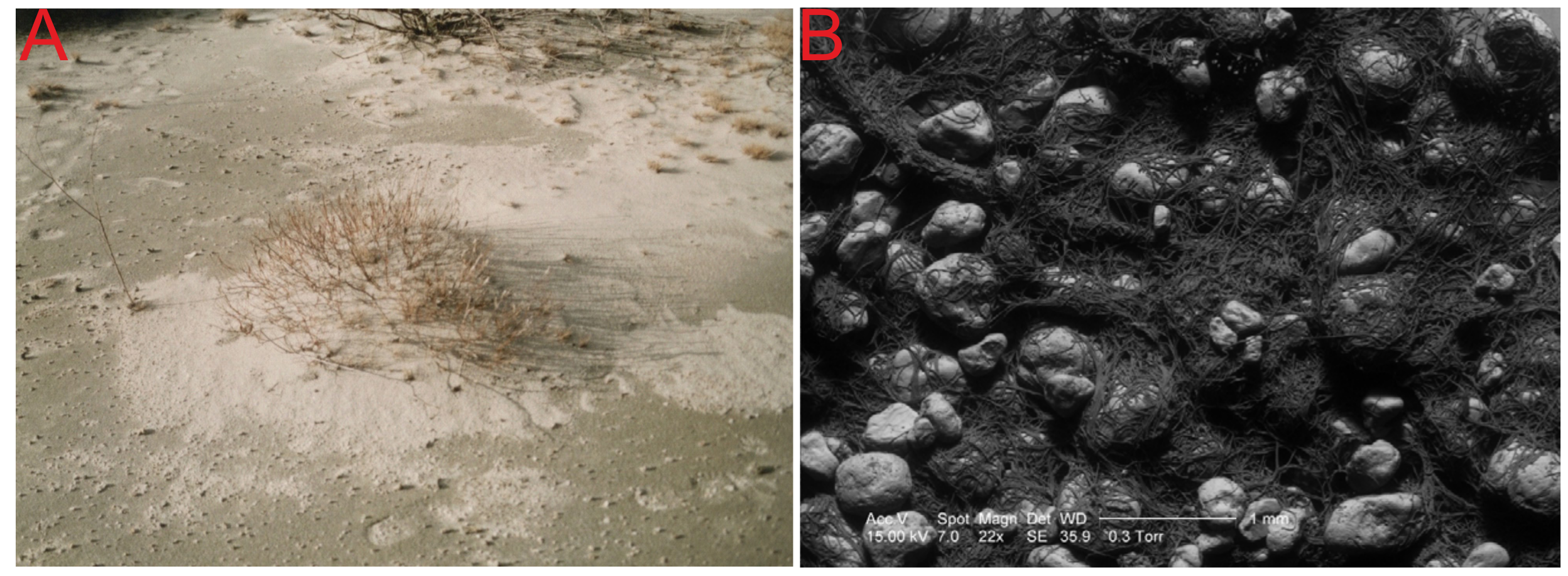
(A) Sand colonisation by algae; (B) Algal net binding sand grains and stabilising loose sand (SEM photograph).
Figure 3.
(A) Sand colonisation by algae; (B) Algal net binding sand grains and stabilising loose sand (SEM photograph).

Figure 4.
The trapping of allochthonous organic matter by Salix arenaria.

Figure 5.
Principal component analysis (PCA), with data pooled for the five-plot study (PC1 × PC2 ordination; the biplot graphic).
Figure 5.
Principal component analysis (PCA), with data pooled for the five-plot study (PC1 × PC2 ordination; the biplot graphic).

Figure 6.
Principal component analyses (PCAs), with data pooled for the five research plots (PC1 × PC2 ordination). The included variables represent the percentage shares of dominant species in plant cover in the studied plots (the biplot graphic).
Figure 6.
Principal component analyses (PCAs), with data pooled for the five research plots (PC1 × PC2 ordination). The included variables represent the percentage shares of dominant species in plant cover in the studied plots (the biplot graphic).

Figure 7.
Accumulation of allogenic substances in the hollow site.

Figure 8.
Relationships between biomass and soil features: (A) The phytomass of dominant species in plots: P.p—Politrychym piliferum, C.c—Corynephorus canescens, S.ar.—Salix arenaria, K.g.—Koeleria glauca, S.ac.—Salix acutifolia, P.s.—Pinus sylvestris; (B) soil profiles; (C) contents of phosphorus in organic/humus horizons; (D) the content of Corg., Nt in selected horizons; (E) soil reaction in humus horizons (A).

Figure 9.
The soil patches under a single specimen.


Table 1.
Environmental conditions and features of plots.
| Numbers of Plots | General Description |
|---|---|
| Plot I | Located on a flattened surface (deflation field) between two low (relative elevations 1–1.6 m) hillocks composed of aeolian sands. Unconsolidated and loose sand with rare vegetation (Figure 1: I, Table 2 *), with active aeolian processes. Soil: initial loose soils (Leptosols). |
| Plot II | Located on a gentle slope of a dune rise, with a relative height of 80–150 cm above the flattened surface. Loose sand partly stabilised by Polytrichum piliferum (Figure 1: II). Low intensity of aeolian processes. Soil: initial loose soils (Leptosols). |
| Plot III | Located on a flattened surface. Weakly expressed nanodepressions. An accumulation of plant detritus was observed, collected by rainwater in small ridges; this was associated with areas characterised by well-developed moss and algae. Stabilised by the turf of P. piliferum and clumps of Salix arenaria (Figure 1: III). Soil: initial loose soils (Leptosols) where there are no plants and soils weakly developed from loose materials (Arenosols). |
| Plot IV | Located on the flattened top of the aeolian ridge and its slope. The surfaces are stable and grassed by Koeleria gluca (Figure 1: IV). There are no destructive aeolian processes. Soil: weakly developed from loose sandy materials (Arenosols). |
| Plot V | Located on the upper part of the slope of the aeolian ridge of the eastern exposition. This surface is the most stable, and the soil was divided into different subhorizons (especially organic horizon) under Pinus sylvestris (Figure 1: V). Soil: weakly developed from loose materials (Arenosols). |
* Occurrence and percentage share of particular species (surface area covered) on the plots are presented in Table 2.
Table 2.
Percentage share of species (surface area covered) on research plots.
| Vegetation and Other Elements | Research Plots [%] | ||||
|---|---|---|---|---|---|
| I | II | III | IV | V | |
| Corynephorus canescens (L.) P.Beauv. | 9.83 | 1.94 | - | - | - |
| Koeleria glauca (Schrad.) DC. | - | 1.55 | 0.21 | 65.66 | 68.4 |
| Polytrichum piliferum Hedw. | 2.11 | 38.71 | 65.6 | 15.95 | 1.79 |
| Salix arenaria L. | 2.38 | 13.8 | 12.61 | 8.42 | 16.43 |
| Salix acutifolia Willd. | 1.25 | 0.84 | 1.47 | - | - |
| Pinus sylvestris L. | 0.21 | 0.29 | 2.23 | - | 9.05 |
| Juniperus communis L. | - | - | 0.05 | - | 0.13 |
| Betula pendula Roth. | - | - | 0.03 | - | - |
| Algae | 48.15 | 7.52 | - | 5.18 | - |
| accumulation of organic matter | - | 7.90 | 6.42 | - | - |
| Bare sand | 36.07 | 27.45 | 11.38 | 4.79 | 4.20 |
| Total | 100 | 100 | 100 | 100 | 100 |
Table 3.
Plant biomass (dry weight) in the algae–mosses communities (Plot I, n = 3).
| Plant Organs | Vegetation Communities and Their Area in m2 | Total in Phytocenosis kg/400 m2 | |||||||||
|---|---|---|---|---|---|---|---|---|---|---|---|
| C. canescens [3.32 m2] | P. piliferum [8.44 m2] | Salix arenaria [9.54 m2] | Salix acutifolia [5.03 m2] | Pinus sylvestris [0.85 m2] | |||||||
| [g/m2] | [kg]- in Community | [g/m2] | [kg]- in Community | [g/m2] | [kg]- in Community | [g/m2] | [kg]- in Community | [g/m2] | [kg]- in Community | ||
| Aboveground biomass: | 10.40 | 0.41 | 76.6 * | 0.65 * | 428.9 | 4.09 | 20.1 | 0.10 | 22.71 | 0.019 | 5.269 |
| leaves | - ** | - | - | - | 24.30 | 0.23 | - | - | - | - | |
| needls | - | - | - | - | - | - | - | - | 0.3 | 0.00011 | |
| living branches | - | - | - | - | 367.6 | 3.50 | - | - | 19.70 | 0.017 | |
| dead branches | - | - | - | - | - | - | 20.1 | 0.10 | - | - | |
| annual increment | - | - | - | - | 37.0 | 0.35 | - | - | 2.88 | 0.002 | |
| Underground biomass: | 108.3 | 4.26 | - | - | 466.7 | 4.46 | 200.7 | 1.00 | 17.53 | 0.014 | 9.734 |
| Roots diameter: <1 mm | 108.3 | 4.26 | - | - | 25.8 | 0.25 | - | - | 6.4 | 0.005 | |
| 1–10 mm | - | - | - | - | 320.5 | 3.06 | 6.4 | 0.03 | 11.13 | 0.009 | |
| >10 mm | - | - | - | - | 120.4 | 1.15 | 194.3 | 0.97 | - | - | |
| TOTAL: | 118.7 | 4.67 | 76.6 | 0.65 | 895.6 | 8.55 | 220.8 | 1.1 | 40.24 | 0.033 | 15.003 |
* The whole mass of plants was taken into account; ** a dash in this table and subsequent tables means that no accounts have been done.
Table 4.
Plant biomass (dry weight) in the sand grasslands and willow communities (Plot II, n = 3).
| Plant Organs | Vegetation Communities and Their Area in m2 | Total in Phytocenosis kg/400 m2 | |||||||||
|---|---|---|---|---|---|---|---|---|---|---|---|
| C. canescens [7.79 m2] | Koeleria glauca [6.2 m2] | Polytrichum piliferum ([54.83 m2] | Salix arenaria [55.26 m2] | Salix acutifolia [3.36 m2] | |||||||
| [g/m2] | [kg]- in Community | [g/m2] | [kg]- in Community | [g/m2] | [kg]- in Community | [g/m2] | [kg]- in Community | [g/m2] | [kg]- in Community | ||
| Aboveground biomass: | 10.4 | 0.08 | 29.0 | 0.18 | 84.3 | 13.05 | 610.2 | 33.72 | 101.3 | 0.34 | 47.37 |
| leaves | - | - | - | - | 179.7 | 9.93 | 43 | 0.14 | |||
| living branches | - | - | - | - | - | - | 388.1 | 21.45 | 19.70 | 0.07 | |
| dead branches | - | - | - | - | - | - | - | - | 38.6 | 0.13 | |
| annual increment | - | - | - | - | - | - | 42.4 | 2.34 | - | - | |
| Underground biomass: | 108.3 | 0.84 | 163.0 | 1.01 | - | - | 2813.2 | 155.46 | 588.3 | 1.98 | 159.29 |
| Roots diameter: <1 mm | 108.3 | 0.84 | 163.0 | 1.01 | - | - | 141.6 | 7.82 | - | - | |
| 1–10 mm | - | - | - | - | - | - | 2130.1 | 117.71 | 12.5 | 0.04 | |
| >10 mm | - | - | - | - | - | - | 541.5 | 29.92 | 575.8 | 1.93 | |
| TOTAL: | 118.7 | 0.92 | 192.0 | 1.19 | 84.3 | 13.05 | 3423.4 | 188.97 | 689.6 | 2.32 | 206.66 |
Table 5.
Plant biomass (dry weight) in the pine–willow–mosses communities (Plot III, n = 3).
| Plant Organs | Vegetation Communities and Their Area in m2 | Total in Phytocenosis kg/400 m2 | |||||||
|---|---|---|---|---|---|---|---|---|---|
| Koeleria glauca [0.84 m2] | Polytrichum piliferum [262.5 m2] | Salix arenaria [50.44 m2] | Pinus sylvestris [8.94 m2] | ||||||
| [g/m2] | [kg]- in Community | [g/m2] | [kg]- in Community | [g/m2] | [kg]- in Community | [g/m2] | [kg]- in Community | ||
| Aboveground biomass: | 20.0 | 0.02 | 112.8 | 29.61 | 1715.1 | 86.51 | 5500.1 | 49.17 | 165.31 |
| leaves | - | - | - | - | 53.9 | 2.72 | - | - | |
| needls | - | - | - | - | - | - | 504.2 | 4,51 | |
| living branches | - | - | - | - | 1649.6 | 83.21 | 1785.2 | 15.96 | |
| trunk | - | - | - | - | - | - | 2485.6 | 22.22 | |
| annual increment | - | - | - | - | 11.6 | 0.58 | 211.2 | 1.89 | |
| Plant litter | - | - | - | - | - | - | 513.9 | 4,59 | |
| Underground biomass: | 116.0 | 0.10 | - | - | 732.2 | 36.93 | 2585.5 | 23.11 | 60.14 |
| Roots diameter: <1 mm | 116.0 | 0.10 | - | - | 70.8 | 3.57 | 123.5 | 1.10 | |
| 1–10 mm | - | - | - | - | 305.4 | 15.40 | 870.2 | 7.78 | |
| >10 mm | - | - | - | - | 356.0 | 17.96 | 1591.8 | 14.23 | |
| TOTAL: | 136.0 | 0.12 | 112.8 | 29.61 | 2447.3 | 123.44 | 8085.6 | 72.28 | 225.45 |
Table 6.
Plant biomass (dry weight) in the sand grassland–mosses–willow communities (Plot IV, n = 3).
Table 6.
Plant biomass (dry weight) in the sand grassland–mosses–willow communities (Plot IV, n = 3).
| Plant Organs | Vegetation Communities and Their Area in m2 | Total in Phytocenosis kg/400 m2 | |||||
|---|---|---|---|---|---|---|---|
| Koeleria glauca [262.67 m2] | Polytrichum piliferum [63.82 m2] | Salix arenaria [33.65 m2] | |||||
| [g/m2] | [kg]- in Community | [g/m2] | [kg]- in Community | [g/m2] | [kg]- in Community | ||
| Aboveground biomass: | 86.9 | 22.83 | 63.7 | 4.07 | 252.4 | 8.49 | 35.39 |
| leaves | - | - | - | - | 44.6 | 1.50 | |
| living branches | - | - | - | - | 183.3 | 6.17 | |
| Annual increment | - | - | - | - | 14.9 | 0.50 | |
| Plant litter | - | - | - | - | 9.6 | 0.32 | |
| Underground biomass: | 87.2 | 22.90 | - | - | 182.5 | 6.14 | 29.04 |
| Roots diameter: <1 mm | 87.2 | 22.90 | - | - | 17.9 | 0.60 | |
| 1–10 mm | - | - | - | - | 101.6 | 3.42 | |
| >10 mm | - | - | - | - | 63.0 | 2.12 | |
| TOTAL: | 174.1 | 45.73 | 63.7 | 4.07 | 434.9 | 14.63 | 64.43 |
Table 7.
Plant biomass (dry weight) in the willow–pine–sand grassland communities (Plot V, n = 3).
| Plant Organs | Vegetation Communities and Their Area in m2 | Total in Phytocenosis kg/400 m2 | |||||||
|---|---|---|---|---|---|---|---|---|---|
| Koeleria glauca [273.8 m2] | Polytrichum piliferum [7.88 m2] | Salix arenaria [65.73 m2] | Pinus sylvestris [36.2 m2] | ||||||
| [g/m2] | [kg]- in Community | [g/m2] | [Kg]- In Community | [g/m2] | [kg]- in Community | [g/m2] | [kg]- in Community | ||
| Aboveground biomass: | 98.8 | 27.05 | 116.1 | 0.91 | 2258.2 | 148.43 | 2007.8 | 72.69 | 249.08 |
| leaves | - | - | - | - | 599.5 | 39.41 | - | - | |
| needls | - | - | - | - | - | - | 122.1 | 4.42 | |
| trunk | - | - | - | - | - | - | 1245.5 | 45.09 | |
| living branches | - | - | - | - | 1543.1 | 101.43 | 378.6 | 13.71 | |
| Dead branches | - | - | - | - | - | - | - | - | |
| Annual increment | - | - | - | - | 101.7 | 6.68 | 10.7 | 0.39 | |
| Plant litter | - | - | - | - | 13.9 | 0.91 | 250.9 | 9.08 | |
| Underground biomass: | 215.9 | 59.11 | - | - | 732.2 | 48.12 | 1147.0 | 41.53 | 148.76 |
| Roots diameter: <1 mm | 215.9 | 59.11 | - | - | 70.8 | 4.65 | 221.7 | 8.03 | |
| 1–10 mm | - | - | - | - | 305.4 | 20.07 | 485.1 | 17.56 | |
| >10 mm | - | - | - | - | 356.0 | 23.40 | 440.2 | 15.94 | |
| TOTAL: | 314.7 | 86.16 | 116.1 | 0.91 | 2990.4 | 196.55 | 3154.8 | 114.22 | 397.84 |
Table 8.
Grain size distribution of soil samples.
| Vegetation/Genetic Horizons | Deepth [cm] | Color According to Munsell | Texture [mm] | |||||
|---|---|---|---|---|---|---|---|---|
| Dry | Wet | >1 | 1.0–0.5 | 0.5–0.25 | 0.25–0.1 | <0.1 | ||
| very coarse | coarse | medium | fine | very fine | ||||
| Algal crust | ||||||||
| OA | 0–1 | 10YR 4/1 | 10YR 2/1 | 0.1 | 31.7 | 49.5 | 15.0 | 3.7 |
| AC | 1–5 | 10YR 6/6 | 10YR 5/6 | 0.1 | 11.0 | 63.4 | 24.7 | 0.8 |
| C | 5–60 | 10YR 7/3 | 10YR 6/4 | 0.7 | 27.0 | 57.6 | 14.5 | 0.2 |
| Polytrichum piliferum | ||||||||
| A | 3–7 | 10YR 4/2 | 10YR 3/1 | 0.0 | 14.8 | 60.2 | 22.2 | 0.8 |
| Salix arenaria (16 y.) | ||||||||
| A | 0–7 | 10YR 3/2 | 10YR 2/1 | 0.0 | 23.0 | 54.7 | 20.0 | 2.3 |
| AC | 7–22 | 10YR 5/4 | 10YR 4/5 | 0.1 | 17.3 | 61.9 | 20.0 | 0.7 |
| C | 27–60 | 10YR 7/3 | 10YR 6/4 | 0.1 | 16.2 | 58.1 | 24.4 | 1.2 |
| Salix acutifolia (21 y.) | ||||||||
| A | 0–13 | 10YR 4/2 | 10YR 3/1 | 0.1 | 20.8 | 55.2 | 21.5 | 2.4 |
| B(fe) | 13–27 | 10YR 5/4 | 10YR 4/3 | 0.4 | 20.3 | 58.7 | 20.2 | 0.4 |
| BC | 27–60 | 10YR 6/4 | 10YR 5/4 | 0.4 | 27.4 | 59.3 | 12.7 | 0.2 |
| Pinus sylvestris (26 y.) | ||||||||
| AE | 0–11 | 10YR 5/2 | 10YR 3/2 | 0.0 | 25.1 | 58.9 | 14.2 | 1.8 |
| AC | 11–17 | 10YR 5/3 | 10YR 4/3 | 0.5 | 27.6 | 56.4 | 14.2 | 1.3 |
| C | 17–30 | 10YR 6/4 | 10YR 5/4 | 0.4 | 29.6 | 53.2 | 16.2 | 0.6 |
| Koeleria glauca | ||||||||
| OA | 0–8 | 10YR 5/2 | 10YR 4/1 | 0.0 | 6.4 | 50.1 | 41.3 | 2.2 |
| IIA1/C1…A8/C8b | 8–37 | 10YR 6/2 | 10YR 5/2 | 0.0 | 6.9 | 56.0 | 36.7 | 0.4 |
| III Ab | 37–40 | 10YR 6/2 | 10YR 4/2 | 0.0 | 0.3 | 51.1 | 47.5 | 1.1 |
| C | 4o-60 | 10YR 6/2 | 10YR 5/2 | 0.0 | 5.5 | 71.6 | 22.8 | 0.1 |
Table 9.
Selected chemical properties of soil under the dominant species (n = 3) in the research plots.
Table 9.
Selected chemical properties of soil under the dominant species (n = 3) in the research plots.
| Vegetation | Horyzont | Depth [cm] | Loss Ignition [%] | Corg [%] | Nt [%] | C/N | Pavial. [mg/kg] | Hh cmol(+)*kg−1 | pH | |
|---|---|---|---|---|---|---|---|---|---|---|
| H2O | KCl | |||||||||
| Algal crust | OA | 0–1 | 2.87 | 1.10 | 0.060 | 18 | 10.41 | 1.59 | 5.1 | 4.5 |
| A | 1–5 | 1.29 | 0.41 | 0.025 | 16 | 3.81 | 0.94 | 5.9 | 4.9 | |
| C | 5–60 | 0.33 | 0.19 | 0.010 | 19 | 2.22 | 0.29 | 5.9 | 5.1 | |
| Polytrichum piliferum | OA | 0–2 | 14.80 | 8.49 | 0.292 | 29 | 47.44 | 5.49 | 4.9 | 4.1 |
| A | 2–7 | 1.39 | 0.62 | 0.029 | 21 | 16.12 | 0.96 | 5.5 | 4.7 | |
| C | 7–60 | 0.62 | 0.22 | 0.013 | 17 | 2.13 | 0.39 | 4.7 | 4.5 | |
| Corynephorus canescens | OA | 0–4 | 0.61 | 0.28 | 0.021 | 13 | 4.32 | 1.52 | 4.9 | 4.2 |
| C | 4–60 | 0.28 | 0.18 | 0.009 | 20 | 4.30 | 0.24 | 6.3 | 5.4 | |
| Koeleria glauca | OA | 0–8 | 1.02 | 0.75 | 0.031 | 24 | 24.10 | 0.90 | 5.9 | 4.9 |
| IIA1C1...A8C8b * | 8–37 | 0.34 | 0.18 | 0.017 | 11 | 17.12 | 0.38 | 6.2 | 5.8 | |
| IIIAb | 37–40 | 0.33 | 0.25 | 0.014 | 18 | 19.18 | 0.38 | 6.3 | 5.8 | |
| C | 40–60 | 0.28 | 0.18 | 0.011 | 16 | 15.16 | 0.38 | 6.1 | 5.8 | |
| Salix arenaria | O (Ol/f/h) | 2–0 | 24.00 | 12.30 | 0.492 | 25 | 36.21 | 6.91 | 5.6 | 4.9 |
| A | 0–7 | 1.98 | 1.42 | 0.072 | 20 | 14.29 | 1.81 | 5.6 | 4.6 | |
| AC | 7–22 | 0.48 | 0.33 | 0.015 | 22 | 12.42 | 0.64 | 5.5 | 4.8 | |
| C | 22–60 | 0.33 | 0.17 | 0.006 | 28 | 27.12 | 0.39 | 5.8 | 5.0 | |
| Salix acutifolia | Ol | 4–2 | 82.50 | 49.20 | 1.560 | 32 | 6.45 | 26.43 | 5.5 | 5.1 |
| Of/h | 2–0 | 21.90 | 11.50 | 0.558 | 20 | 6.89 | 7.05 | 5.8 | 5.2 | |
| A | 0–13 | 1.45 | 0.59 | 0.040 | 15 | 2.69 | 0.83 | 6.1 | 5.4 | |
| B(fe) | 13–27 | 1.01 | 0.34 | 0.022 | 15 | 19.13 | 0.92 | 5.9 | 5.2 | |
| BC | 27–60 | 0.58 | 0.17 | 0.007 | 24 | 25.11 | 0.53 | 5.8 | 5.2 | |
| Pinus sylvestris | Ol | 9–6 | 96.00 | 49.40 | 0.903 | 54 | 5.32 | 50.92 | 3.9 | 3.2 |
| Of | 5–2 | 62.10 | 32.12 | 0.615 | 52 | 6.49 | 16.38 | 4.4 | 3.7 | |
| Oh | 2–1 | 44.20 | 19.51 | 0.508 | 38 | 65.23 | 5.12 | 4.3 | 3.4 | |
| AE | 0–11 | 0.77 | 0.43 | 0.015 | 29 | 31.09 | 1.07 | 5.5 | 4.8 | |
| AC | 11–17 | 0.63 | 0.2‘7 | 0.008 | 34 | 5.21 | 0.69 | 5.4 | 4.7 | |
| C | 17–60 | 0.63 | 0.22 | 0.005 | 44 | 3.44 | 0.53 | 5.4 | 4.8 | |
* Buried horizons.
Table 10.
Total content of selected major elements (n = 3) in mineral horizons of soils in plots.
| Vegetation | Horyzont | Depth [cm] | Total Content [mg/kg] | |||||||
|---|---|---|---|---|---|---|---|---|---|---|
| Ca | Mg | K | Na | P | Fe | Al | Zn | |||
| Algae | OA | 0–4 | 310 | 515 | 5113 | 1766 | 180 | 286 | 1090 | 97 |
| Polytrichum piliferum | A | 3–7 | 450 | 280 | 2700 | 660 | 110 | 7750 | 10,400 | 6 |
| C | 7–60 | 220 | 180 | 600 | 450 | 89 | 4700 | 14,800 | 180 | |
| Corynephorus canescens | OA | 0–4 | 340 | 145 | 210 | 490 | 220 | 3800 | 11,200 | 9 |
| C | 4–60 | 330 | 130 | 240 | 620 | 110 | 1335 | 9800 | 6 | |
| Koeleria glauca | OA | 0–8 | 330 | 230 | 2500 | 650 | 70 | 4000 | 11,300 | 65 |
| IIA1C1...A8C8b | 8–37 | 280 | 100 | 220 | 610 | 120 | 2300 | 9200 | 40 | |
| IIIAb | 37–40 | 540 | 290 | 2900 | 850 | 160 | 4400 | 1900 | 27 | |
| C | 40–60 | 400 | 150 | 3700 | 790 | 70 | 1900 | 12,300 | 70 | |
| Salix arenaria | A | 0–7 | 310 | 140 | 2100 | 490 | 220 | 3800 | 14,000 | 9 |
| C | 22–60 | 340 | 130 | 2400 | 620 | 110 | 1300 | 12,200 | 6 | |
| Salix acutifolia | A | 0–13 | 840 | 290 | 2800 | 680 | 60 | 3800 | 14,100 | 290 |
| B(fe) | 13–27 | 290 | 130 | 2600 | 620 | 30 | 1500 | 13,100 | 9 | |
| BC | 27–60 | 210 | 120 | 2500 | 590 | 40 | 1500 | 9800 | 9 | |
| Pinus sylvestris | AE | 0–11 | 750 | 240 | 2750 | 740 | 70 | 250 | 14,000 | 650 |
| AC | 11–17 | 310 | 140 | 2600 | 770 | 50 | 1500 | 13,000 | 70 | |
| C | 17–60 | 360 | 150 | 2200 | 630 | 0,00 | 1100 | 8800 | 20 | |
Publisher’s Note: MDPI stays neutral with regard to jurisdictional claims in published maps and institutional affiliations. |
© 2021 by the authors. Licensee MDPI, Basel, Switzerland. This article is an open access article distributed under the terms and conditions of the Creative Commons Attribution (CC BY) license (http://creativecommons.org/licenses/by/4.0/).
Share and Cite
MDPI and ACS Style
Rahmonov, O.; Skreczko, S.; Rahmonov, M. Changes in Soil Features and Phytomass during Vegetation Succession in Sandy Areas. Land 2021, 10, 265. https://doi.org/10.3390/land10030265
AMA Style
Rahmonov O, Skreczko S, Rahmonov M. Changes in Soil Features and Phytomass during Vegetation Succession in Sandy Areas. Land. 2021; 10(3):265. https://doi.org/10.3390/land10030265
Chicago/Turabian StyleRahmonov, Oimahmad, Sylwia Skreczko, and Małgorzata Rahmonov. 2021. "Changes in Soil Features and Phytomass during Vegetation Succession in Sandy Areas" Land 10, no. 3: 265. https://doi.org/10.3390/land10030265
Note that from the first issue of 2016, this journal uses article numbers instead of page numbers. See further details here.