
Spatiotemporal Evolution Analysis of Habitat Quality under High-Speed Urbanization: A Case Study of Urban Core Area of China Lin-Gang Free Trade Zone (2002–2019)


Abstract
:1. Introduction
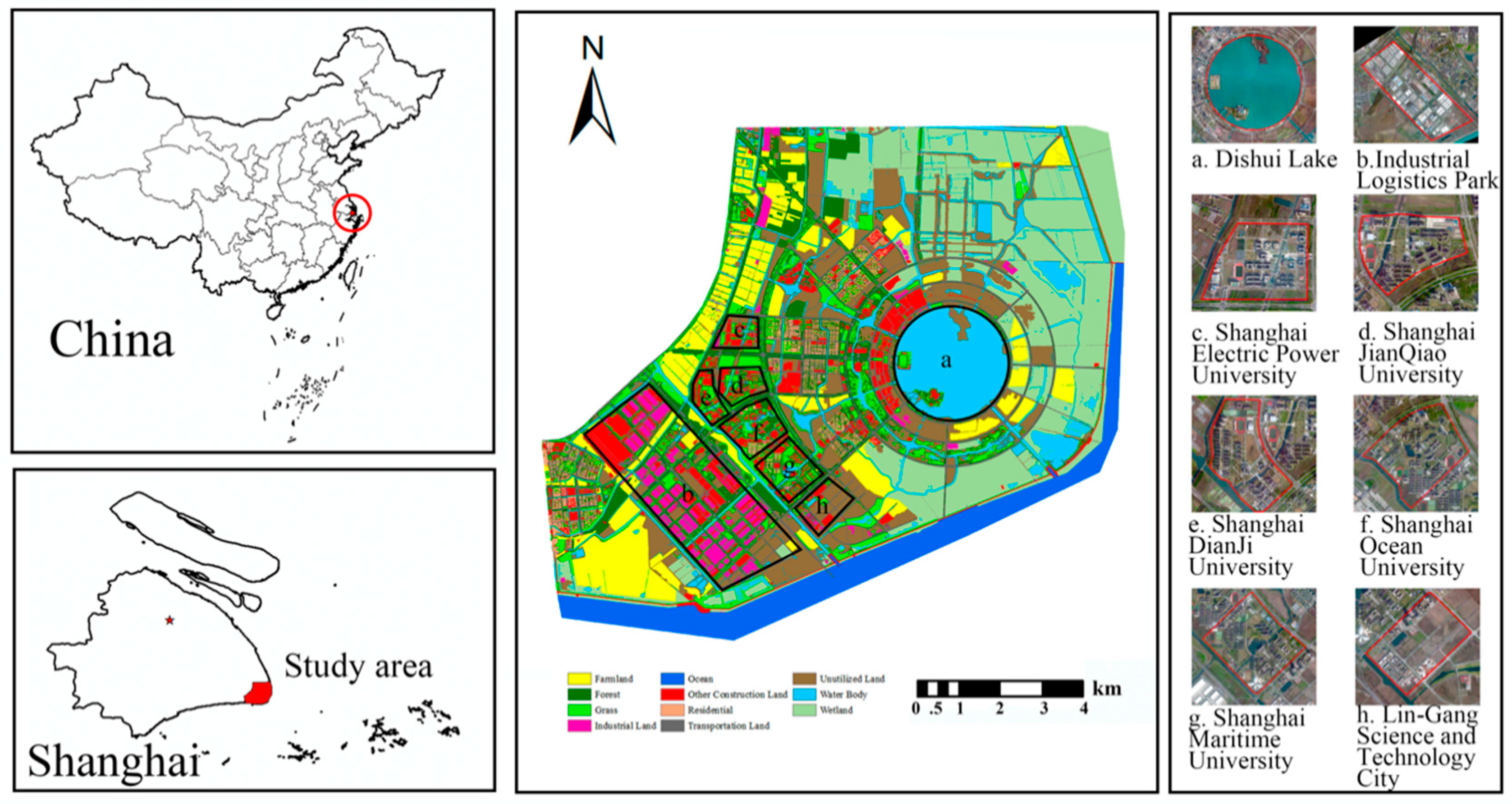
2. Study Area
3. Research Methods
3.1. Subsection Remote Sensing Image Classification
3.2. Habitat Quality Assessment
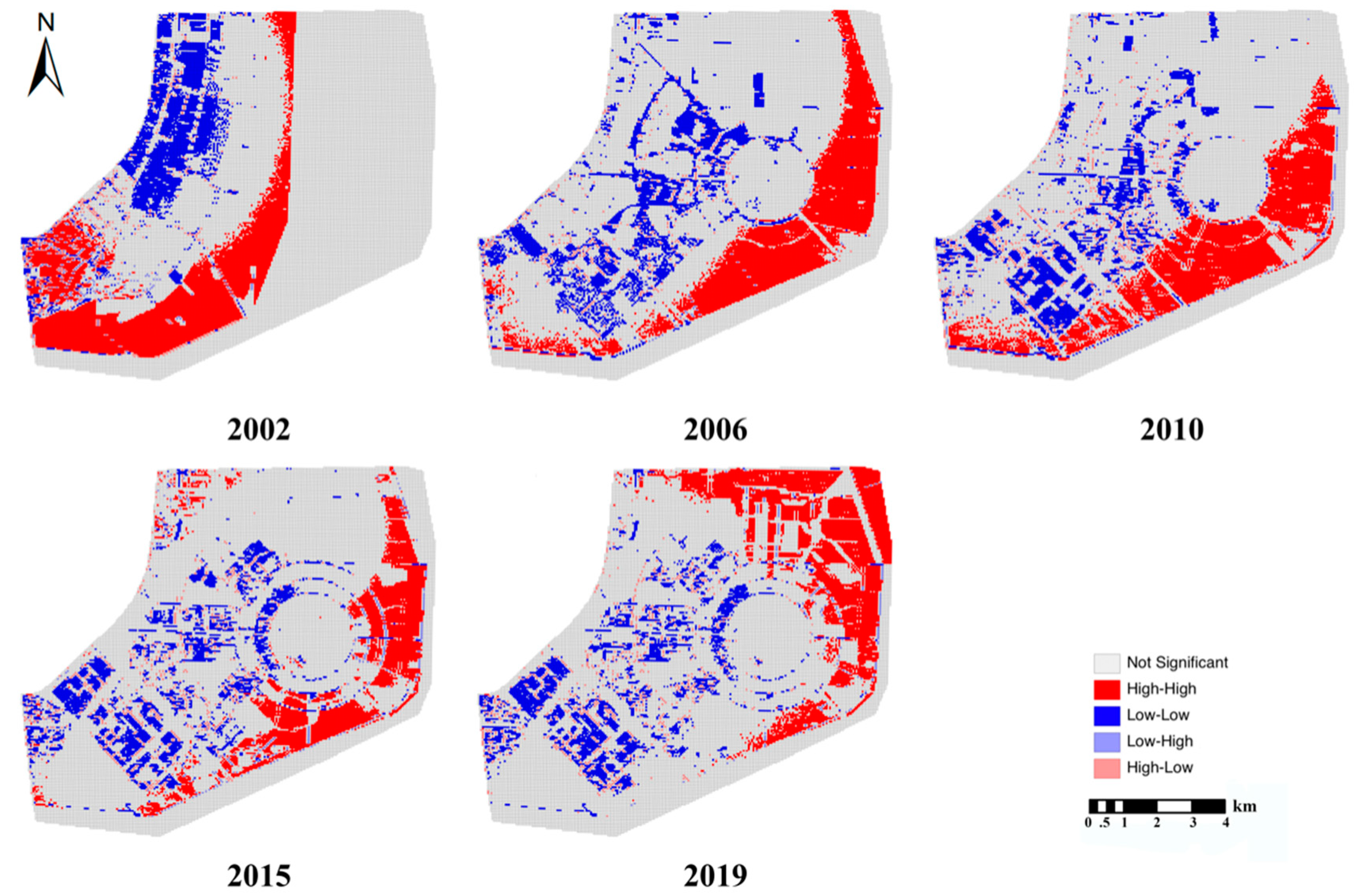
3.3. Spatial Autocorrelation Analysis
3.4. Landscape Pattern Analysis
4. Results Analysis
4.1. InVEST-HQ Model Parameter Selection
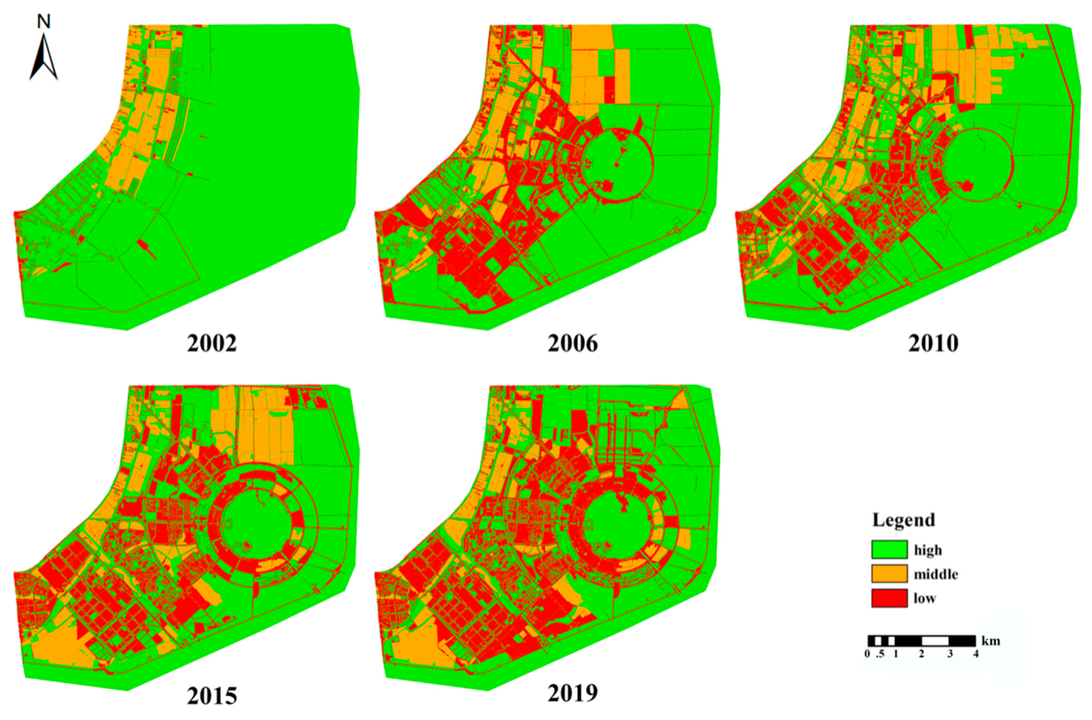
4.2. Spatial Distribution of Habitat Quality
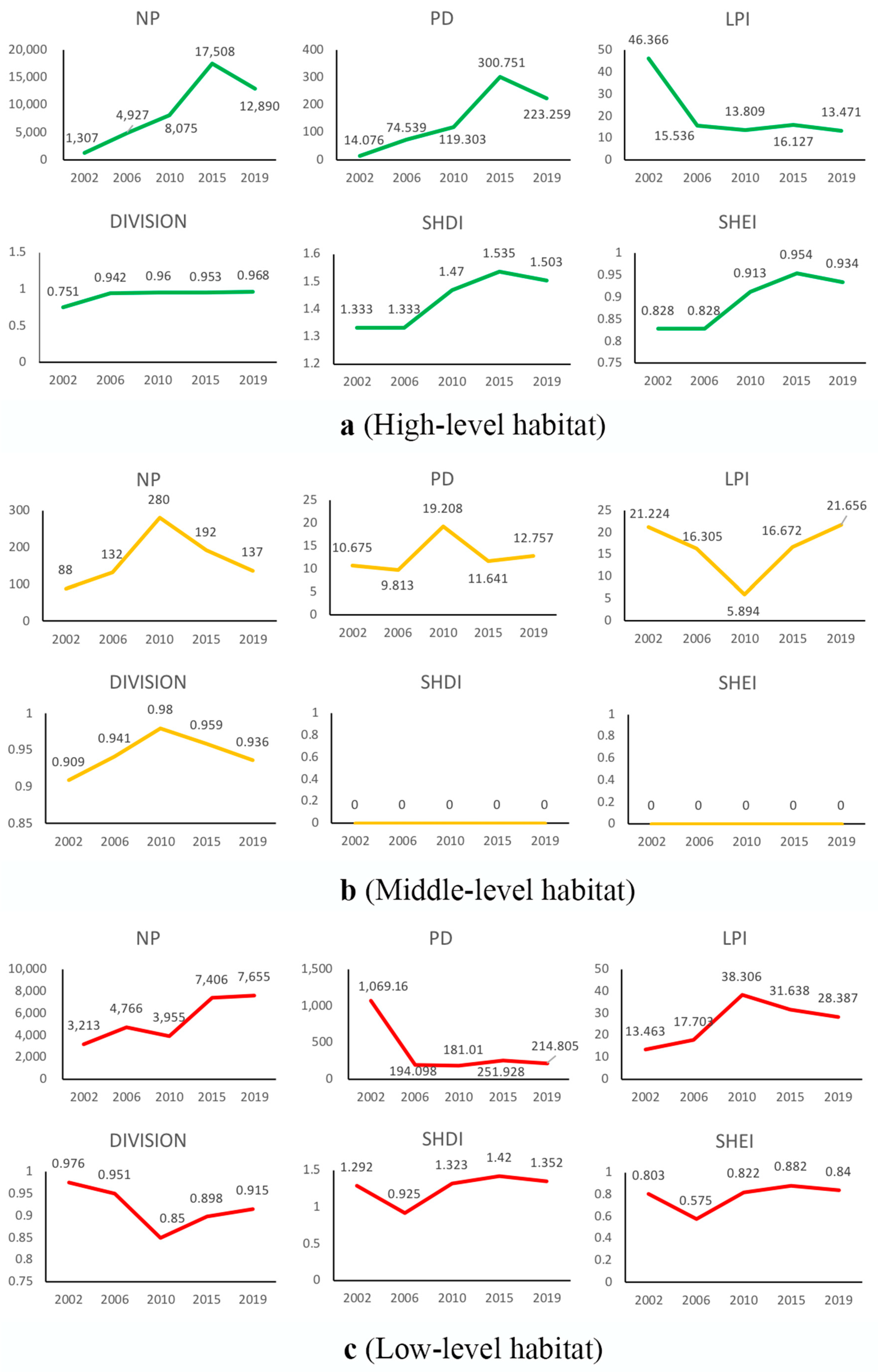
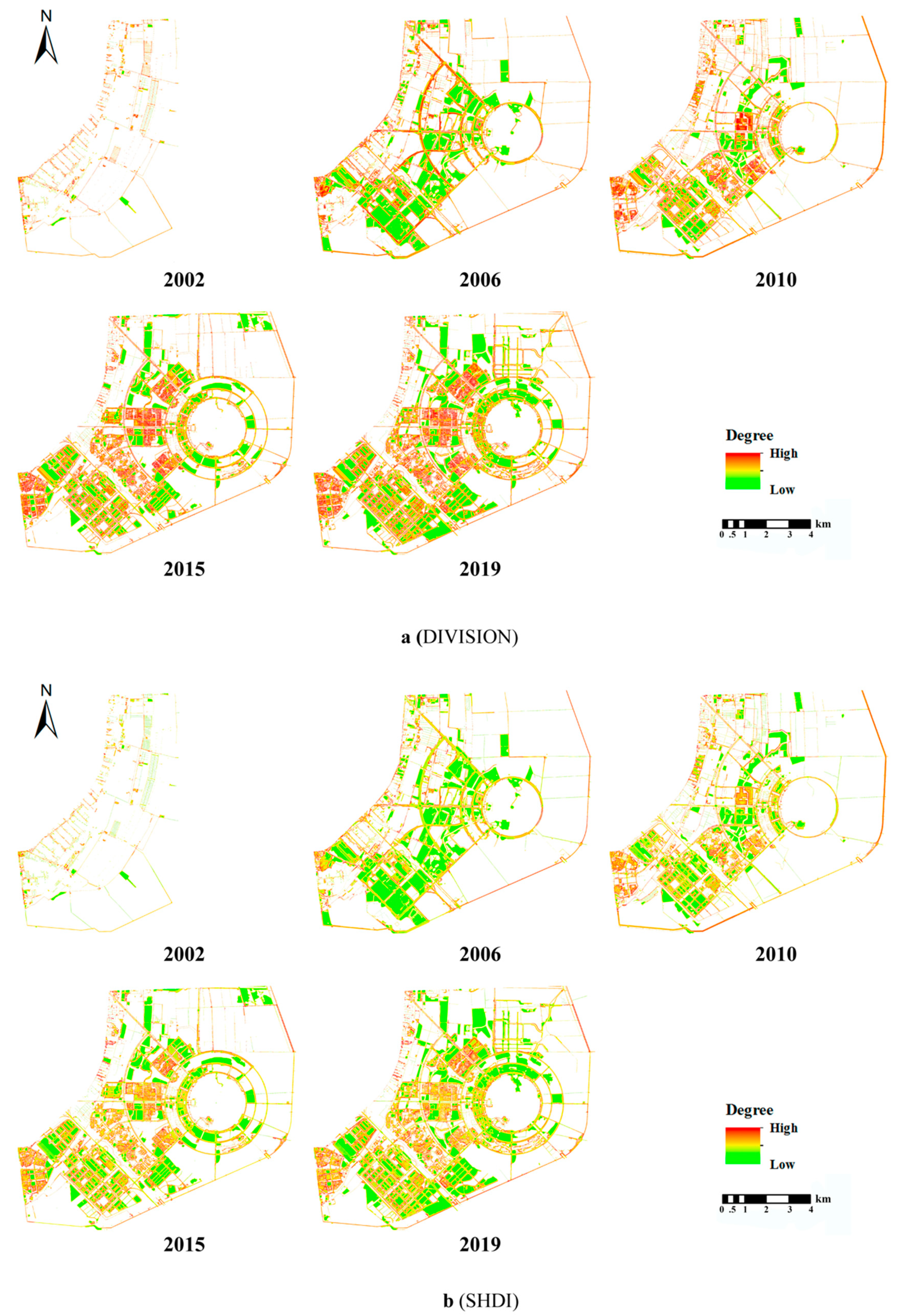
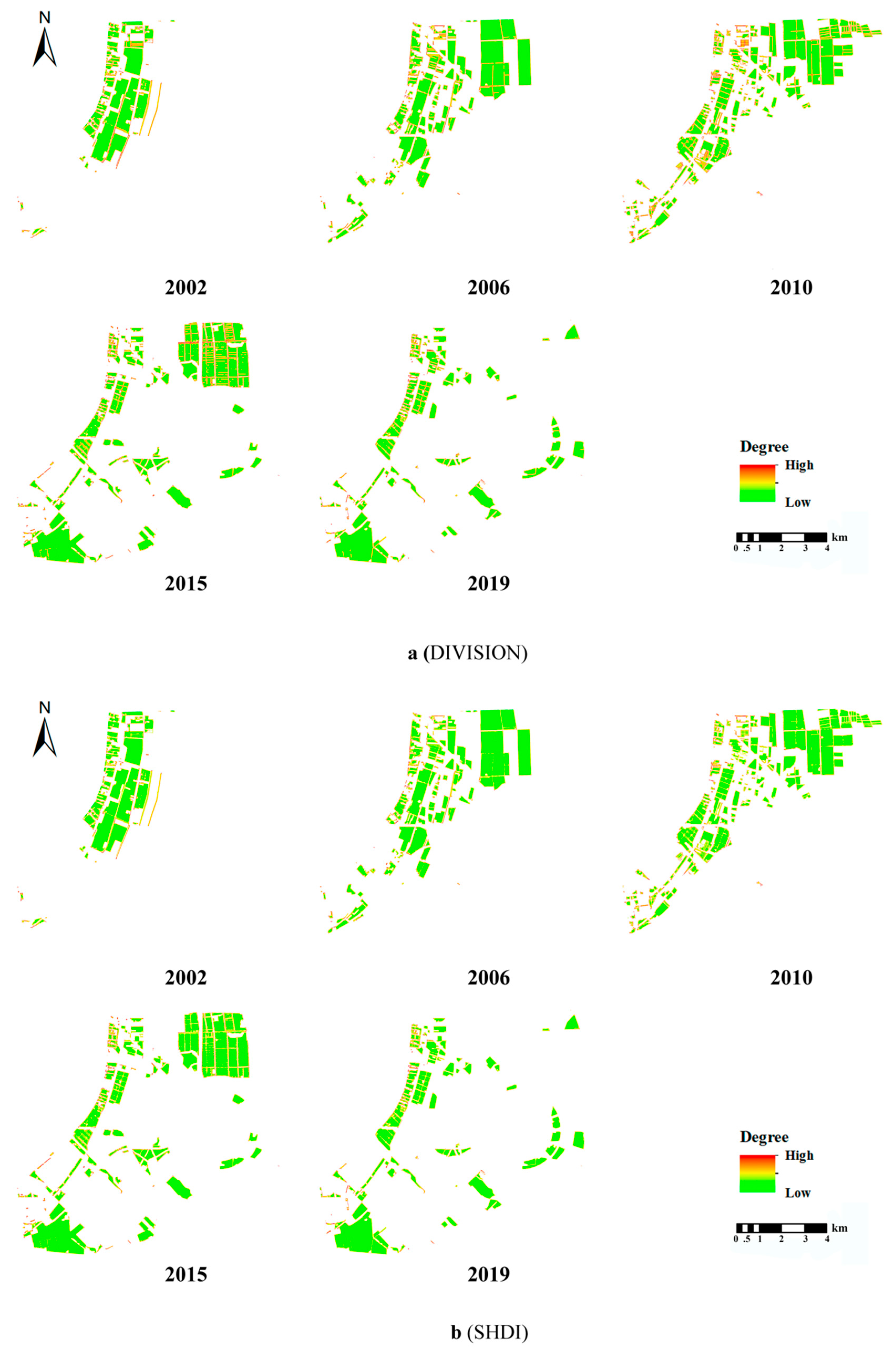
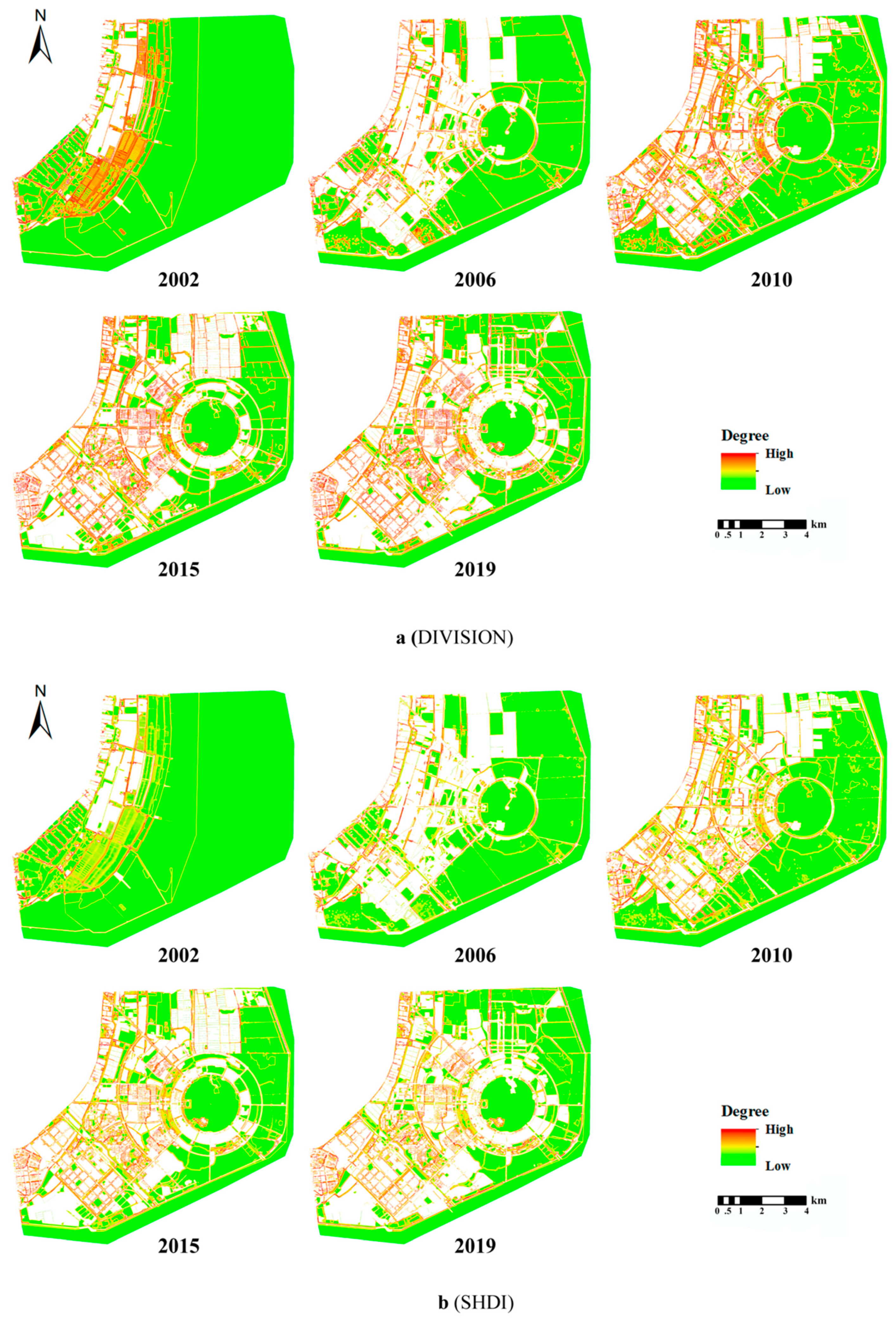
4.3. Landscape Pattern Analysis
4.4. Analysis of Habitat Landscape Pattern Based on the Moving Window Model
5. Conclusions
Author Contributions
Funding
Institutional Review Board Statement
Informed Consent Statement
Data Availability Statement
Conflicts of Interest
References
- Lyu, R.; Zhang, J.; Xu, M.; Li, J. Impacts of urbanization on ecosystem services and their temporal relations: A case study in Northern Ningxia, China. Land Use Policy 2018, 77, 163–173. [Google Scholar] [CrossRef]
- Sun, L.; Chen, J.; Li, Q.; Huang, D. Dramatic uneven urbanization of large cities throughout the world in recent decades. Nat. Commun. 2020, 11. [Google Scholar] [CrossRef]
- Cui, E.; Ren, L.; Sun, H. Evaluation of variations and affecting factors of eco-environmental quality during urbanization. Environ. Sci. Pollut. Res. 2015, 22, 3958–3968. [Google Scholar] [CrossRef]
- Yao, L.; Liu, J.; Wang, R.; Yin, K.; Han, B. A qualitative network model for understanding regional metabolism in the context of Social-Economic-Natural Complex Ecosystem theory. Ecol. Inform. 2015, 26, 29–34. [Google Scholar] [CrossRef]
- Han, B.; Liu, H.; Wang, R. Urban ecological security assessment for cities in the Beijing-Tianjin-Hebei metropolitan region based on fuzzy and entropy methods. Ecol. Model. 2015, 318, 217–225. [Google Scholar] [CrossRef]
- Pullanikkatil, D.; Palamuleni, L.G.; Ruhiiga, T.M. Land use/land cover change and implications for ecosystems services in the Likangala River Catchment, Malawi. Phys. Chem. Earth Parts A/B/C 2016, 93, 96–103. [Google Scholar] [CrossRef]
- Zhu, E.; Deng, J.; Zhou, M.; Gan, M.; Jiang, R.; Wang, K.; Shahtahmassebi, A.R. Carbon emissions induced by land-use and land-cover change from 1970 to 2010 in Zhejiang, China. Sci. Total Environ. 2019, 646, 930–939. [Google Scholar] [CrossRef]
- Zhu, E.; Deng, J.; Wang, H.; Wang, K.; Huang, L.; Zhu, G.; Belete, M.; Shahtahmassebi, A.R. Identify the optimization strategy of nitrogen fertilization level based on trade-off analysis between rice production and greenhouse gas emission. J. Clean. Prod. 2019, 239, 118060. [Google Scholar] [CrossRef]
- Paruelo, J.M.; Burke, I.C.; Lauenroth, W.K. Land-use impact on ecosystem functioning in eastern Colorado, USA. Glob. Chang. Biol. 2001, 7, 631–639. [Google Scholar] [CrossRef]
- Dresser, C.; Inc, M. Evaluation of Integrated Suface Water and Groundwater Modeling Tools. Water Resour. Res. 2001, 35. [Google Scholar]
- Goldstein, J.H.; Caldarone, G.; Duarte, T.K.; Ennaanay, D.; Hannahs, N.; Mendoza, G.; Polasky, S.; Wolny, S.; Daily, G.C. Integrating ecosystem-service tradeoffs into land-use decisions. Proc. Natl. Acad. Sci. USA 2012, 109, 7565–7570. [Google Scholar] [CrossRef] [PubMed] [Green Version]
- Terrado, M.; Sabater, S.; Chaplin-Kramer, B.; Mandle, L.; Ziv, G.; Acuña, V. Model development for the assessment of terrestrial and aquatic habitat quality in conservation planning. Sci. Total Environ. 2016, 540, 63–70. [Google Scholar] [CrossRef] [Green Version]
- Zhu, C.; Zhang, X.; Zhou, M.; He, S.; Gan, M.; Yang, L.; Wang, K. Impacts of urbanization and landscape pattern on habitat quality using OLS and GWR models in Hangzhou, China. Ecol. Indic. 2020, 117, 106654. [Google Scholar] [CrossRef]
- De Mendonça, M.J.C.; Sachsida, A.; Loureiro, P.R.A. A study on the valuing of biodiversity: The case of three endangered species in Brazil. Ecol. Econ. 2003, 46, 9–18. [Google Scholar] [CrossRef]
- Hamer, A.J. Accessible habitat delineated by a highway predicts landscape-scale effects of habitat loss in an amphibian community. Landsc. Ecol. 2016, 31, 2259–2274. [Google Scholar] [CrossRef]
- Balasooriya, B.L.W.K.; Samson, R.; Mbikwa, F.; Vitharana, U.W.A.; Boeckx, P.; Van Meirvenne, M. Biomonitoring of urban habitat quality by anatomical and chemical leaf characteristics. Environ. Exp. Bot. 2009, 65, 386–394. [Google Scholar] [CrossRef]
- Partyka, M.L.; Peterson, M.S. Habitat quality and salt-marsh species assemblages along an anthropogenic estuarine landscape. J. Coast. Res. 2008, 24, 1570–1581. [Google Scholar] [CrossRef]
- Wu, Y.; Tao, Y.; Yang, G.; Ou, W.; Pueppke, S.; Sun, X.; Chen, G.; Tao, Q. Impact of land use change on multiple ecosystem services in the rapidly urbanizing Kunshan City of China: Past trajectories and future projections. Land Use Policy 2019, 85, 419–427. [Google Scholar] [CrossRef]
- Leh, M.D.K.; Matlock, M.D.; Cummings, E.C.; Nalley, L.L. Quantifying and mapping multiple ecosystem services change in West Africa. Agric. Ecosyst. Environ. 2013, 165, 6–18. [Google Scholar] [CrossRef]
- Mushet, D.M.; Neau, J.L.; Euliss, N.H. Modeling effects of conservation grassland losses on amphibian habitat. Biol. Conserv. 2014, 174, 93–100. [Google Scholar] [CrossRef]
- Sherrouse, B.C.; Semmens, D.J.; Clement, J.M. An application of Social Values for Ecosystem Services (SolVES) to three national forests in Colorado and Wyoming. Ecol. Indic. 2014, 36, 68–79. [Google Scholar] [CrossRef]
- Pérez-Vega, A.; Mas, J.F.; Ligmann-Zielinska, A. Comparing two approaches to land use/cover change modeling and their implications for the assessment of biodiversity loss in a deciduous tropical forest. Environ. Model. Softw. 2012, 29, 11–23. [Google Scholar] [CrossRef]
- Boumans, R.; Roman, J.; Altman, I.; Kaufman, L. The multiscale integrated model of ecosystem services (MIMES): Simulating the interactions of coupled human and natural systems. Ecosyst. Serv. 2015, 12, 30–41. [Google Scholar] [CrossRef]
- Benocci, R.; Brambilla, G.; Bisceglie, A.; Zambon, G. Eco-acoustic indices to evaluate soundscape degradation due to human intrusion. Sustainability 2020, 12, 455. [Google Scholar] [CrossRef]
- Winkler, D.; Bidló, A.; Bolodár-Varga, B.; Erdő, Á.; Horváth, A. Long-term ecological effects of the red mud disaster in Hungary: Regeneration of red mud flooded areas in a contaminated industrial region. Sci. Total Environ. 2018, 644, 1292–1303. [Google Scholar] [CrossRef]
- Mcdonald, R.I.; Kareiva, P.; Forman, R.T.T. The implications of current and future urbanization for global protected areas and biodiversity conservation. Biol. Conserv. 2008, 141, 1695–1703. [Google Scholar] [CrossRef]
- Seto, K.C.; Güneralp, B.; Hutyra, L.R. Global forecasts of urban expansion to 2030 and direct impacts on biodiversity and carbon pools. Proc. Natl. Acad. Sci. USA 2012, 109, 16083–16088. [Google Scholar] [CrossRef] [Green Version]
- Güneralp, B.; Seto, K.C. Futures of global urban expansion: Uncertainties and implications for biodiversity conservation. Environ. Res. Lett. 2013, 8. [Google Scholar] [CrossRef]
- Swenson, J.J.; Franklin, J. The effects of future urban development on habitat fragmentation in the Santa Monica Mountains. Landsc. Ecol. 2000, 15, 713–730. [Google Scholar] [CrossRef]
- Li, T.; Shilling, F.; Thorne, J.; Li, F.; Schott, H.; Boynton, R.; Berry, A.M. Fragmentation of China’s landscape by roads and urban areas. Landsc. Ecol. 2010, 25, 839–853. [Google Scholar] [CrossRef] [Green Version]
- Krauss, J.; Bommarco, R.; Guardiola, M.; Heikkinen, R.K.; Helm, A.; Kuussaari, M.; Lindborg, R.; Öckinger, E.; Pärtel, M.; Pino, J.; et al. Habitat fragmentation causes immediate and time-delayed biodiversity loss at different trophic levels. Ecol. Lett. 2010, 13, 597–605. [Google Scholar] [CrossRef] [Green Version]
- Scolozzi, R.; Geneletti, D. A multi-scale qualitative approach to assess the impact of urbanization on natural habitats and their connectivity. Environ. Impact Assess. Rev. 2012, 36, 9–22. [Google Scholar] [CrossRef]
- Botequilha Leitão, A.; Ahern, J. Applying landscape ecological concepts and metrics in sustainable landscape planning. Landsc. Urban Plan. 2002, 59, 65–93. [Google Scholar] [CrossRef]
- Moser, D.; Zechmeister, H.G.; Plutzar, C.; Sauberer, N.; Wrbka, T.; Grabherr, G. Landscape patch shape complexity as an effective measure for plant species richness in rural landscapes. Landsc. Ecol. 2002, 17, 657–669. [Google Scholar] [CrossRef]
- Li, H.; Wu, J. Use and misuse of landscape indices. Landsc. Ecol. 2004, 19, 389–399. [Google Scholar] [CrossRef] [Green Version]
- Uuemaa, E.; Antrop, M.; Roosaare, J.; Marja, R.; Mander, Ü. Landscape metrics and indices: An overview of their use in landscape research. Living Rev. Landsc. Res. 2009, 3, 1–28. [Google Scholar] [CrossRef]
- Béliveau, M.; Germain, D.; Ianăş, A.N. Fifty-year spatiotemporal analysis of landscape changes in the Mont Saint-Hilaire UNESCO Biosphere Reserve (Quebec, Canada). Environ. Monit. Assess. 2017, 189. [Google Scholar] [CrossRef] [PubMed]
- Mcgarigal, K.; Cushman, S.; Neel, M. FRAGSTATS: Spatial Pattern Analysis Program for Categorical Maps; University of Massachusetts: Amherst, MA, USA, 2002; ISBN 0278-4807. [Google Scholar]
- Pătru-Stupariu, I.; Stupariu, M.S.; Tudor, C.A.; Grădinaru, S.R.; Gavrilidis, A.; Kienast, F.; Hersperger, A.M. Landscape fragmentation in Romania’s Southern Carpathians: Testing a European assessment with local data. Landsc. Urban Plan. 2015, 143, 1–8. [Google Scholar] [CrossRef]
- Du, X.; Huang, Z. Ecological and environmental effects of land use change in rapid urbanization: The case of hangzhou, China. Ecol. Indic. 2017, 81, 243–251. [Google Scholar] [CrossRef]
- Miller, J.R.; Hobbs, R.J. Habitat Restoration—Do we know what were doing? Restor. Ecol. 2007, 15, 382–390. [Google Scholar] [CrossRef]
- Sharp, R.; Tallis, H.T.; Ricketts, T.; Guerry, A.D.; Wood, S.A.; Chaplin-Kramer, R.; Nelson, E.; Enaanay, D.; Wolny, S.; Olwero, N.; et al. InVEST User Guide. Natl. Cap. Proj. 2018, 21. [Google Scholar]
- Wang, Q.; Yang, S.; Zheng, M.; Han, F.; Ma, Y. Effects of vegetable fields on the spatial distribution patterns of metal(Loid)s in soils based on GIS and Moran’s I. Int. J. Environ. Res. Public Health 2019, 16, 4095. [Google Scholar] [CrossRef] [PubMed] [Green Version]
- Ma, F.; Liu, F.; Sun, Q.; Wang, W.; Li, X. Measuring and spatio-temporal evolution for the late-development advantage in China’s provinces. Sustainability 2018, 10, 2773. [Google Scholar] [CrossRef] [Green Version]
- Jia, Y.; Tang, X.; Liu, W. Spatial-temporal evolution and correlation analysis of ecosystem service value and landscape ecological risk in wuhu city. Sustainability 2020, 12, 2803. [Google Scholar] [CrossRef] [Green Version]
- Wang, H.; Tang, L.; Qiu, Q.; Chen, H. Assessing the impacts of urban expansion on habitat quality by combining the concepts of land use, landscape, and habitat in two Urban agglomerations in China. Sustainability 2020, 12, 4346. [Google Scholar] [CrossRef]
- Yirigui, Y.; Lee, S.W.; Nejadhashemi, A.P.; Herman, M.R.; Lee, J.W. Relationships between riparian forest fragmentation and biological indicators of streams. Sustainability 2019, 11, 2870. [Google Scholar] [CrossRef] [Green Version]
- Kowe, P.; Mutanga, O.; Odindi, J.; Dube, T. A quantitative framework for analysing long term spatial clustering and vegetation fragmentation in an urban landscape using multi-temporal landsat data. Int. J. Appl. Earth Obs. Geoinf. 2020, 88, 102057. [Google Scholar] [CrossRef]
- Kong, F.; Nakagoshi, N. Spatial-temporal gradient analysis of urban green spaces in Jinan, China. Landsc. Urban Plan. 2006, 78, 147–164. [Google Scholar] [CrossRef]
- Announcement of the General Planning of the Land and Space of the Lingang New Area of the China (Shanghai) Pilot Free Trade Zone. 2020. Available online: http://ghzyj.sh.gov.cn/ghgs/20200622/c1d9cde4f2ee4b60a345c2dc2598335e.html (accessed on 30 October 2020).
- Bai, L.; Xiu, C.; Feng, X.; Liu, D. Influence of urbanization on regional habitat quality:a case study of Changchun City. Habitat Int. 2019, 93. [Google Scholar] [CrossRef]
- Sun, X.; Jiang, Z.; Liu, F.; Zhang, D. Monitoring spatio-temporal dynamics of habitat quality in Nansihu Lake basin, eastern China, from 1980 to 2015. Ecol. Indic. 2019, 102, 716–723. [Google Scholar] [CrossRef]
- Aneseyee, A.B.; Noszczyk, T.; Soromessa, T.; Elias, E. The InVEST habitat quality model associated with land use/cover changes: A qualitative case study of the Winike Watershed in the Omo-Gibe Basin, Southwest Ethiopia. Remote Sens. 2020, 12, 1103. [Google Scholar] [CrossRef] [Green Version]
- Shanghai Lingang New City Management Measures. 2004. Available online: http://www.moj.gov.cn/Department/content/2004-03/10/595_210181.html (accessed on 30 October 2020).
- Land and Space Master Plan of Pudong New Area. 2017. Available online: http://hd.ghzyj.sh.gov.cn/xxgk/ghjh/202003/t20200303_960552.html (accessed on 30 October 2020).
- Shi, Q.; Gao, J.; Wang, X.; Ren, H.; Cai, W.; Wei, H. Temporal and spatial variability of carbon emission intensity of urban residential buildings: Testing the effect of economics and geographic location in China. Sustainability 2020, 12, 2695. [Google Scholar] [CrossRef] [Green Version]
- Wang, C.; Wang, G.; Dai, L.; Liu, H.; Li, Y.; Zhou, Y.; Chen, H.; Dong, B.; Lv, S.; Zhao, Y. Diverse usage of waterbird habitats and spatial management in Yancheng coastal wetlands. Ecol. Indic. 2020, 117, 106583. [Google Scholar] [CrossRef]


| Time Period | LULC | Farmland | Forest Land | Grassland | Industrial Land | Ocean | Other Construction Land | Residential Land | Transportation Land | Unutilized Land | Water Body | Wetland |
|---|---|---|---|---|---|---|---|---|---|---|---|---|
| 2002–2006 | Farmland | 4.591 | 0.870 | 0.394 | 0.003 | 1.415 | 0.001 | 0.071 | 0.015 | 0.259 | 1.961 | 3.877 |
| Forest Land | 1.324 | 3.730 | 0.246 | 0.009 | 0.032 | 0.006 | 0.149 | 0.077 | 0.079 | 0.310 | 0.149 | |
| Grassland | 0.195 | 0.611 | 0.647 | 0.010 | 0.442 | 0.007 | 0.067 | 0.021 | 0.088 | 1.721 | 1.462 | |
| Industrial Land | 0.104 | 0.074 | 0.028 | 0.016 | 0.003 | 0.003 | 0.007 | 0.001 | 0.018 | 0.089 | 0.071 | |
| Ocean | 0.000 | 0.000 | 0.000 | 0.000 | 10.335 | 0.000 | 0.000 | 0.000 | 0.000 | 0.001 | 0.000 | |
| Other Construction Land | 0.020 | 0.300 | 0.114 | 0.020 | 0.363 | 0.002 | 0.038 | 0.020 | 0.012 | 0.233 | 0.215 | |
| Residential Land | 0.035 | 0.258 | 0.035 | 0.026 | 0.000 | 0.001 | 0.383 | 0.019 | 0.033 | 0.016 | 0.004 | |
| Transportation Land | 0.441 | 0.652 | 0.418 | 0.020 | 0.689 | 0.004 | 0.121 | 0.362 | 0.129 | 1.023 | 1.289 | |
| Unutilized Land | 1.336 | 1.404 | 1.360 | 0.072 | 1.326 | 0.010 | 0.217 | 0.126 | 0.374 | 5.491 | 5.162 | |
| Water Body | 0.204 | 0.211 | 0.150 | 0.002 | 4.757 | 0.002 | 0.018 | 0.012 | 0.030 | 2.254 | 2.219 | |
| Wetland | 0.002 | 0.000 | 0.145 | 0.001 | 23.787 | 0.000 | 0.003 | 0.033 | 0.011 | 1.664 | 8.970 | |
| 2006–2010 | Farmland | 8.223 | 1.394 | 0.281 | 0.033 | 0.000 | 0.015 | 0.119 | 0.115 | 1.104 | 0.160 | 3.133 |
| Forest Land | 1.063 | 1.777 | 0.518 | 0.009 | 0.017 | 0.042 | 0.078 | 0.594 | 1.424 | 0.175 | 0.217 | |
| Grassland | 1.197 | 1.303 | 1.676 | 0.037 | 0.002 | 0.098 | 0.154 | 0.570 | 4.314 | 0.538 | 1.853 | |
| Industrial Land | 0.069 | 0.071 | 0.102 | 0.187 | 0.000 | 0.004 | 0.013 | 0.015 | 0.640 | 0.010 | 0.015 | |
| Ocean | 0.000 | 0.001 | 0.000 | 0.000 | 9.389 | 0.014 | 0.000 | 0.001 | 0.002 | 0.005 | 0.003 | |
| Other Construction Land | 0.227 | 0.237 | 0.380 | 0.075 | 0.061 | 0.839 | 0.092 | 0.364 | 1.431 | 0.070 | 0.172 | |
| Residential Land | 0.077 | 0.093 | 0.135 | 0.014 | 0.000 | 0.012 | 0.175 | 0.051 | 0.218 | 0.017 | 0.129 | |
| Transportation Land | 0.843 | 0.817 | 0.722 | 0.037 | 0.010 | 0.221 | 0.131 | 2.993 | 2.486 | 0.291 | 0.590 | |
| Unutilized Land | 1.224 | 0.100 | 0.781 | 0.014 | 0.002 | 0.042 | 0.018 | 0.147 | 3.146 | 0.340 | 0.940 | |
| Water Body | 0.349 | 0.291 | 0.271 | 0.003 | 0.000 | 0.008 | 0.028 | 0.089 | 0.932 | 7.187 | 3.569 | |
| Wetland | 0.185 | 0.027 | 0.402 | 0.006 | 0.855 | 0.041 | 0.001 | 0.211 | 1.180 | 1.065 | 23.994 | |
| 2010–2015 | Farmland Land | 8.106 | 0.388 | 1.083 | 0.001 | 0.000 | 0.051 | 0.032 | 0.508 | 1.132 | 0.484 | 4.707 |
| Forest Land | 1.062 | 2.737 | 1.719 | 0.017 | 0.000 | 0.234 | 0.068 | 1.225 | 0.333 | 0.164 | 0.308 | |
| Grassland | 0.787 | 0.944 | 3.576 | 0.029 | 0.004 | 0.289 | 0.058 | 0.925 | 0.998 | 0.366 | 0.812 | |
| Industrial Land | 0.096 | 0.066 | 0.379 | 0.836 | 0.000 | 0.267 | 0.019 | 0.104 | 0.187 | 0.044 | 0.188 | |
| Ocean | 0.000 | 0.001 | 0.001 | 0.000 | 9.359 | 0.004 | 0.000 | 0.000 | 0.001 | 0.000 | 0.117 | |
| Other Construction Land | 0.750 | 0.348 | 1.000 | 0.099 | 0.014 | 2.098 | 0.032 | 0.653 | 1.048 | 0.152 | 0.412 | |
| Residential Land | 0.113 | 0.056 | 0.361 | 0.010 | 0.000 | 0.106 | 0.609 | 0.152 | 0.239 | 0.048 | 0.001 | |
| Transportation Land | 0.610 | 0.826 | 1.358 | 0.047 | 0.000 | 0.630 | 0.084 | 4.641 | 0.668 | 0.218 | 1.317 | |
| Unutilized Land | 1.707 | 0.271 | 1.220 | 0.087 | 0.000 | 0.077 | 0.013 | 0.385 | 1.189 | 0.362 | 3.222 | |
| Water Body | 0.308 | 0.127 | 0.330 | 0.001 | 0.023 | 0.015 | 0.002 | 0.117 | 0.193 | 7.964 | 2.085 | |
| Wetland | 1.038 | 0.149 | 0.716 | 0.000 | 0.016 | 0.175 | 0.005 | 0.429 | 0.765 | 2.927 | 14.798 | |
| 2015–2019 | Farmland Land | 8.403 | 0.272 | 0.176 | 0.001 | 0.000 | 0.013 | 0.012 | 0.055 | 0.950 | 0.043 | 0.816 |
| Forest Land | 0.142 | 5.364 | 1.158 | 0.013 | 0.000 | 0.196 | 0.110 | 0.754 | 0.141 | 0.054 | 0.121 | |
| Grassland | 0.564 | 0.609 | 4.087 | 0.018 | 0.000 | 0.262 | 0.069 | 0.405 | 0.592 | 0.085 | 0.742 | |
| Industrial Land | 0.003 | 0.016 | 0.023 | 1.890 | 0.000 | 0.174 | 0.005 | 0.045 | 0.033 | 0.000 | 0.150 | |
| Ocean | 0.000 | 0.000 | 0.000 | 0.000 | 7.743 | 0.011 | 0.000 | 0.001 | 0.000 | 0.024 | 0.065 | |
| Other Construction Land | 0.044 | 0.105 | 0.164 | 0.115 | 0.002 | 4.719 | 0.057 | 0.409 | 0.322 | 0.009 | 0.123 | |
| Residential Land | 0.006 | 0.061 | 0.038 | 0.001 | 0.000 | 0.188 | 1.303 | 0.070 | 0.027 | 0.003 | 0.001 | |
| Transportation Land | 0.060 | 0.823 | 0.501 | 0.102 | 0.015 | 0.607 | 0.117 | 8.105 | 0.317 | 0.026 | 0.205 | |
| Unutilized Land | 2.528 | 0.364 | 2.064 | 0.030 | 0.000 | 0.399 | 0.021 | 0.404 | 4.905 | 0.353 | 3.628 | |
| Water Body | 0.629 | 0.106 | 0.244 | 0.005 | 0.000 | 0.013 | 0.002 | 0.035 | 0.239 | 9.691 | 1.046 | |
| Wetland | 4.113 | 0.147 | 0.333 | 0.011 | 1.724 | 0.024 | 0.000 | 0.116 | 1.008 | 0.876 | 14.121 |
| Threat Factors | Maximum Distance of Influence | Weight | Type of Decay over Space |
|---|---|---|---|
| Farmland | 4 | 0.7 | Linear |
| Transportation Land | 3 | 1 | Exponential |
| Residential Land | 5 | 0.7 | Exponential |
| Other Construction Land | 8 | 0.6 | Exponential |
| Industrial Land | 8 | 1 | Exponential |
| Unutilized Land | 6 | 0.5 | Exponential |
| LULC | Habitat Suitability | Farmland | Transportation Land | Residential Land | Other Construction Land | Industrial Land | Unutilized Land |
|---|---|---|---|---|---|---|---|
| Forest Land | 1 | 0.5 | 0.7 | 0.7 | 0.9 | 0.9 | 0.6 |
| Grassland | 1 | 0.7 | 0.8 | 0.8 | 0.1 | 0.1 | 0.5 |
| Ocean | 0.9 | 0.5 | 0.2 | 0.2 | 0.8 | 0.8 | 0.5 |
| Transportation Land | 0 | 0 | 0 | 0 | 0.2 | 0.2 | 0 |
| Residential Land | 0 | 0 | 0.7 | 0 | 0.4 | 0.4 | 0.5 |
| Farmland | 0.4 | 0 | 0.5 | 0.4 | 0.7 | 0.8 | 0.4 |
| Water Body | 0.7 | 0.7 | 0.3 | 0 | 0.5 | 0.5 | 0.3 |
| Other Construction Land | 0 | 0 | 0 | 0.5 | 0 | 0 | 0 |
| Unutilized Land | 0.2 | 0.5 | 0.7 | 0.7 | 0.8 | 0.8 | 0 |
| Industrial Land | 0 | 0 | 0.3 | 0 | 0.3 | 0 | 0 |
| Wetland | 1 | 0.7 | 0.6 | 0.7 | 0.8 | 0.8 | 0.8 |
| Year | Average Value | Standard Deviation | Area (km2)/Proportion (%) | |||||
|---|---|---|---|---|---|---|---|---|
| High-Level | Middle-Level | Low-Level | ||||||
| 2002 | 0.842 | 0.214 | 92.86 | 89.09 | 8.24 | 7.91 | 3.01 | 2.88 |
| 2006 | 0.681 | 0.363 | 66.11 | 63.42 | 13.45 | 12.91 | 24.55 | 23.56 |
| 2010 | 0.673 | 0.377 | 67.68 | 64.94 | 14.58 | 13.99 | 21.85 | 20.96 |
| 2015 | 0.598 | 0.398 | 58.21 | 55.85 | 16.49 | 15.82 | 29.40 | 28.20 |
| 2019 | 0.582 | 0.406 | 57.74 | 55.39 | 10.74 | 10.30 | 35.64 | 34.19 |
Publisher’s Note: MDPI stays neutral with regard to jurisdictional claims in published maps and institutional affiliations. |
© 2021 by the authors. Licensee MDPI, Basel, Switzerland. This article is an open access article distributed under the terms and conditions of the Creative Commons Attribution (CC BY) license (http://creativecommons.org/licenses/by/4.0/).
Share and Cite
Chen, L.; Wei, Q.; Fu, Q.; Feng, D. Spatiotemporal Evolution Analysis of Habitat Quality under High-Speed Urbanization: A Case Study of Urban Core Area of China Lin-Gang Free Trade Zone (2002–2019). Land 2021, 10, 167. https://doi.org/10.3390/land10020167
Chen L, Wei Q, Fu Q, Feng D. Spatiotemporal Evolution Analysis of Habitat Quality under High-Speed Urbanization: A Case Study of Urban Core Area of China Lin-Gang Free Trade Zone (2002–2019). Land. 2021; 10(2):167. https://doi.org/10.3390/land10020167
Chicago/Turabian StyleChen, Lisu, Qiong Wei, Qiang Fu, and Daolun Feng. 2021. "Spatiotemporal Evolution Analysis of Habitat Quality under High-Speed Urbanization: A Case Study of Urban Core Area of China Lin-Gang Free Trade Zone (2002–2019)" Land 10, no. 2: 167. https://doi.org/10.3390/land10020167