Article

Estimating Water Footprints of Vegetable Crops: Influence of Growing Season, Solar Radiation Data and Functional Unit

by
Betsie Le Roux
1,
Michael Van der Laan
1,*,
Teunis Vahrmeijer
1,2,
John G. Annandale
1 and
Keith L. Bristow
1,3
1
Department of Plant Production and Soil Science, University of Pretoria, Private Bag X20, Hatfield 0028, South Africa
2
Citrus Research International, P.O. Box 28, Nelspruit 1200, South Africa
3
CSIRO Agriculture, PMB Aitkenvale, Townsville 4814, Queensland, Australia
*
Author to whom correspondence should be addressed.
Water 2016, 8(10), 473; https://doi.org/10.3390/w8100473
Submission received: 24 June 2016 / Revised: 19 September 2016 / Accepted: 8 October 2016 / Published: 22 October 2016
(This article belongs to the Special Issue Water Footprint Assessment)

Abstract

:
Water footprint (WF) accounting as proposed by the Water Footprint Network (WFN) can potentially provide important information for water resource management, especially in water scarce countries relying on irrigation to help meet their food requirements. However, calculating accurate WFs of short-season vegetable crops such as carrots, cabbage, beetroot, broccoli and lettuce presented some challenges. Planting dates and inter-annual weather conditions impact WF results. Joining weather datasets of just rainfall, minimum and maximum temperature with ones that include solar radiation and wind-speed affected crop model estimates and WF results. The functional unit selected can also have a major impact on results. For example, WFs according to the WFN approach do not account for crop residues used for other purposes, like composting and animal feed. Using yields in dry matter rather than fresh mass also impacts WF metrics, making comparisons difficult. To overcome this, using the nutritional value of crops as a functional unit can connect water use more directly to potential benefits derived from different crops and allow more straightforward comparisons. Grey WFs based on nitrogen only disregards water pollution caused by phosphates, pesticides and salinization. Poor understanding of the fate of nitrogen complicates estimation of nitrogen loads into the aquifer.

Graphical Abstract

1. Introduction

In many catchments throughout South Africa, water supply no longer meets demand [1]. Climate change, population growth and improved standards of living will exacerbate this even further in the future. Irrigated agriculture uses approximately 40% of South Africa’s exploitable runoff on around 1.7 million hectares of land [2]. Agricultural products account for approximately 6.5% of total South African national exports, approximating 3% of gross domestic product [3]. Nieuwoudt et al. [4] estimated that 90% of vegetable and fruit products are grown under irrigation in South Africa because of low and erratic rainfall and the high value of these crops. Horticulture is therefore highly dependent on the continued availability of irrigation water to remain sustainable. However, surface water resources in South Africa are already almost fully developed, and although alternative sources can still be exploited, it will be done at significantly higher costs than previously [1]. The vulnerability of food production in South Africa was emphasized by the drought of 2015 which was, according to the South African Weather Bureau, the driest calendar year since nationwide recordings started in 1904 [5]. As a result, preliminary estimates on crop production for the 2016 calendar year indicate that production of most crops is expected to decrease [6]. One of the key findings of the Water Resource Reconciliation Strategies for major cities and towns in South Africa, was that little additional surface water can be made available to agriculture in the future, and that many areas are already considering the re-allocation of irrigation water to other users [1]. The “Reconciliation Strategy for the Crocodile West Water Supply System”, for example, suggested that leakages in the distribution network of irrigation water from the Crocodile Catchment should be addressed and that this water be reallocated to augment water requirements of the rapid developments in the Lephalale area or for urban and rural use [7].
Water Footprint (WF) accounting is an emerging approach first proposed by the Water Footprint Network (WFN) in 2002, aiming to better quantify the impacts of human activities on water quantity and quality and guide improved decision making and management. Hoekstra et al. [8] distinguish between “blue”, “green” and “grey” WFs. Surface and underground water resources, which are available to multiple users, are defined as blue water. In a crop production context, blue water consists predominantly of the irrigation water applied. Green water originates from rainfall that is stored in the soil and is only available for evapotranspiration (ET). In order to account for water quality impacts, the WFN [8] proposed the concept of a grey WF, which is the volume of water required to dilute pollutants to naturally occurring levels. Water footprints can indicate water consumption, defined as the loss of water from a particular catchment, for example through evaporation or transfers to other catchments, along the entire production chain per yield of product [8]. Whereas traditionally the focus has been on agricultural producers and the technical aspects of irrigation and drainage to reduce impacts on freshwater resources, WFs further potentially allow water issues to be addressed through regional trade policies and consumer attitudes [9]. Water footprint accounting also has the potential to provide crop water use metrics in an easily understandable way, which can assist farmers to improve the management of their water resources by informing production decisions. If WFs can be established for a number of well-managed farms, these could serve as benchmarks that can be used by other farmers to improve their blue, green and grey water footprint. Efficient use of green water in agriculture is essential to minimize the exploitation of blue water resources for irrigation. Over-irrigation is undesirable, because it can result in water logging, soil salinization, groundwater pollution, leaching of nutrients, and other impacts on the soil [10,11,12].
A number of studies have been conducted on the WFs of various crops, for example the WFN calculated the WFs for several crops from global databases at a 5 by 5 arc minute grid [13]. In South Africa, WFs have been calculated for the cultivation of various crops, including the vegetables cabbage, tomatoes, spinach, potatoes and green beans cultivated under different smallholder irrigation schemes [14], for lucerne as livestock feed for milk production [15], for sugar cane [16] and for the biodiesel crop Jatropha curcas [17]. A product WF was calculated for producing beer by SABMiller in South Africa [18]. WFs have been calculated for agriculture in the Breede Water Management Area [19], and for South Africa as a whole [20]. These studies indicated that WFs can potentially be a useful tool to quantify direct and indirect water use, with its flexibility being particularly advantageous, as it can be applied to various entities, including products, consumers, businesses and catchments [21]. WF were also found useful to assess water used in terms of economic gains and job creation [19], and to inform policy making to improve sustainable development [20]. The importance of calculating WFs with local data and interpreting WFs within the local context has been emphasized [14,15].
The Steenkoppies Aquifer is located west of Tarlton, South Africa, and is a major vegetable producing region in Gauteng. During the 1980s, agricultural activities on the Steenkoppies Aquifer increased dramatically, sourcing irrigation water from the aquifer through boreholes. The discharge of surface water from the aquifer was drastically reduced as a result [22], which caused conflict between farmers on the aquifer and downstream users [23].
This research was conducted as part of a Water Research Commission (WRC) project [
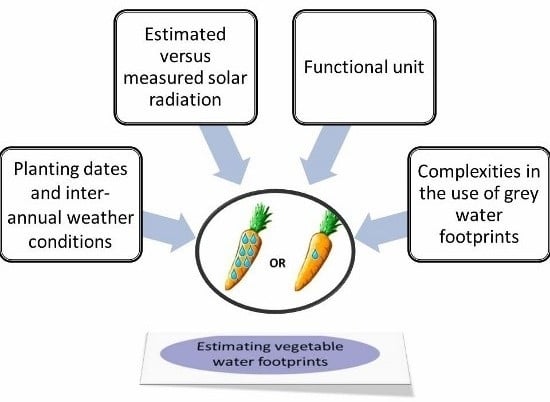
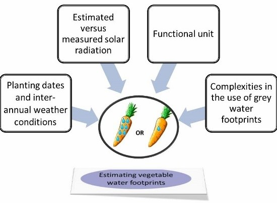
24] on WF accounting, aiming to better understand the potential intricacies involved in calculating WFs of vegetable crops using a case study on the water stressed Steenkoppies Aquifer. In this paper, we report on how WF outcomes are influenced by several factors, including natural variations in weather conditions between growing seasons and between different years. Water footprints are also directly dependent on crop simulation model outputs, which are in turn affected by the quality of parameterisation and input data used, including weather data. Variations in water content between different crops can impact the WFs, which are most commonly expressed as a volume of water used per yield in fresh mass, and we explore the impact of functional units on the results. Finally, some complexities in using the grey WF method are discussed, and aquifer water quality measurements used to challenge the calculation of grey WFs.

2. Materials and Methods

The Steenkoppies Aquifer (Lat: 26.03° S to 26.19° S, Long: 27.65° E to 27.48° E; Altitude 1560–1650 m) is located in a summer rainfall region. Average maximum temperatures range from 19 °C in winter to 25 °C in summer, and average minimum temperatures range from 4 °C in winter to 12 °C in summer [25]. Mean annual rainfall over the past 60 years is 670 mm [25].

2.1. Determining the WFs of Crops on the Steenkoppies Aquifer

Blue, green and grey WFs for the cultivation phase of the major crops grown on the Steenkoppies Aquifer were calculated according to the WFN approach [8]. Carrots (Daucus carota), beetroot (Beta vulgaris), cabbage and broccoli (Brassica oleracea), lettuce (Lactuca sativa), maize (Zea mays) and wheat (Triticum aestivum) are the most important crops cultivated on the Steenkoppies Aquifer. The two grain crops are included here for comparative purposes. On the Steenkoppies Aquifer, these crops are mainly cultivated under pivot or sprinkler irrigation. Evapotranspiration during the cultivation phase is considered to have the highest WF along the supply chain; for example, according to Ridoutt and Pfister [26], the cultivation phase of two food products contributed 97% of the stress weighted WF. The WFN noted the cultivation phase to be the most significant portion of the overall WF of agricultural products [8], because worldwide agriculture is responsible for 86% of total water used [27]. Any water consumed in the pack house and along the supply chain to the consumer was excluded. Water used to raise crop seedlings was also excluded, because this water is often sourced from other catchments and the quantities are relatively small compared to total ET during cultivation. Water embedded in the crop was also excluded, because this only represents about 1% of total crop water use [8].

2.1.1. Crop Water Use Modelling

The data required for blue and green WF calculations were generated using the Soil Water Balance (SWB) crop model [28]. SWB is a mechanistic, daily time-step, generic crop model. Crop growth is simulated to be either water- or radiation-limited. SWB requires daily weather, soil and crop data as inputs. Weather data inputs include rainfall (mm), minimum and maximum temperature (°C), relative humidity (%), solar radiation (MJ·m−2·day−1) and wind speed (m·s−1) and is used to calculate the reference evapotranspiration (ETo) using the Penman-Monteith equation [29]. If wind speed, solar radiation and relative humidity are unavailable, SWB estimates these values according to Food and Agriculture Organization of the United States (FAO) 56 recommendations [29]. Wind speed is assumed to be 2 m·s−1, solar radiation is estimated based on latitude and temperature, and humidity is estimated based on minimum temperatures [28,29]. The SWB model was considered the most appropriate model for this application, because it can simulate growth of a range of different crops, it is able to simulate daily crop water use, has been extensively tested and applied in South Africa, and is relatively simple to use [28,30,31,32,33].
Soil input data used to parameterise and calibrate the SWB model included soil texture and matric potential at full capacity and permanent wilting point (kPa), a drainage factor (0 to 1) and drainage rate (mm·day−1) and maximum rooting depth. For each of the 11 soil layers the following data was parameterised: depth of layer (m), volumetric water content (m3·m−3) at field capacity and permanent wilting point, initial water content (m3·m−3) and bulk density (Mg·m−3).
For each crop SWB provided daily and seasonal ET, irrigation applied and yield data for 10 years from 2004 to 2013. Standard deviations were calculated for irrigation and yield over the 10 years.

2.1.2. Crop Parameters

New crop parameters for carrots, cabbage, beetroot, broccoli and lettuce (Table 1) were recently calibrated for the region based on intensive growth analyses by Vahrmeijer [34]. Trials were done on commercial farms on the Steenkoppies Aquifer under optimal management practices. Cultivars used most commonly by farmers on the Steenkoppies Aquifer for each season were selected for parameterisation. Cabbage cultivars “Tenacity” and “Grandslam”, carrots cultivars “Star 3006” and “Dordogne” and broccoli cultivars “Star 2204” and “Parthenon” were used for summer and winter, respectively. The beetroot cultivar “Red Ace” and lettuce cultivar “Robbenson” was used for all seasons. Parameters that were developed for summer were also applied for spring, except for beetroot which required slightly different parameters in spring, and the parameters developed for winter were also applied for autumn. Crop parameters for maize and wheat were sourced from Annandale et al. [28].

2.1.3. Verification of SWB Results

SWB results were verified by comparing simulated yield and irrigation data (with standard deviations), to independent actual measurements made on eight farms on the Steenkoppies Aquifer. Four replications of 1 m2 plots were demarcated on cropped areas of each farm. Rain gauges were installed within the cropped area to measure Irrigation and rainfall and outside the fields to measure rainfall only. The crops were harvested at the commercial harvesting date and the harvestable portion was weighed to determine yield in terms of both fresh mass and dry matter. The grain crops data were validated by Jovanovic et al. [35], and were included for comparative purposes.

2.1.4. Water Footprint Calculations

Using the verified modelled data and long term simulations from 2004 to 2013, blue and green WFs were calculated according to the WFN approach as given in Equations (1) and (2), respectively [8]:
B l u e   W a t e r   F o o t p r i n t   =   m i n   ( C r o p   E T ,   I r r ) Y i e l d
and
G r e e n   W a t e r   F o o t p r i n t   = [ C r o p   E T     m i n   ( C r o p   E T ,   I r r ) ] Y i e l d
where crop ET is the crop evapotranspiration (mm), Irr (mm) is the total irrigation from planting to harvesting. As per Hoekstra et al. [8], yield in fresh mass was used. Water Footprints were also calculated using yield in dry matter as an alternative (kg·m−2). SWB provided crop ET, irrigation and yield data for all crops over 10 years from 2004 to 2013.
Agricultural activities are commonly associated with water pollution, because of the pesticides and fertilizers and other agrichemicals that are used which can be exported to water bodies. Nitrogen (N) and phosphorus (P) pollution from agriculture has received much attention because of the well-known role these nutrients play in eutrophication of surface water resources [36,37,38,39]. While eutrophication might not become a problem if either N or P are limiting, it is important to minimize the amount of N and P entering our surface and groundwater resources. In an aquatic ecosystem where only P levels are controlled, excess N can still result in eutrophication of water resources further downstream including estuaries and coastal marine ecosystems [39]. Both N and P should therefore be taken into account when calculating grey WFs. Nitrogen is of additional concern, because of the health risks it poses to infants younger than six months (blue baby syndrome) [40]. Inorganic N is usually more mobile than P in soil, because P is adsorbed to clay particles [39,41,42]. Nitrogen pollution can also indirectly mobilise P by oxidising geological pyrite deposits and increasing sulphate levels, which react with iron compounds, causing adsorbed P to be released and mobilised, potentially causing eutrophication [41] Gleeson et al. [43] have also highlighted the need to set groundwater sustainability targets that meet drinking water standards, and this highlights the importance of including N in grey WFs for groundwater. Nitrogen is also the most common agricultural pollutant that has been used for calculating grey WFs [13,44,45,46], which enables comparisons with a wide range of other WF studies reported in the literature. We have therefore used N as the critical pollutant during the cultivation phase to determine grey WFs of the vegetables selected for this study. We also recognise that other pollutants, including P and pesticides, might be more appropriate in other studies.
Grey WFs were determined using Equation (3) given by the WFN [8] as:
G r e y   W a t e r   F o o t p r i n t   = N   L o a d C m a x C n a t   × F W 1
where Cmax and Cnat are the maximum and natural background concentrations of the pollutant respectively. The general standards for N in wastewater of 15 mg·L−1 [47] was taken as Cmax. Cnat is the N concentration of the water if no human influences are present. The aquifer has very low N concentrations, with an average of 0.3 mg·L−1 [48], and therefore does not reflect the expected impacts of the agricultural activities. Thus, average natural N concentrations of the aquifer were considered to represent the natural conditions, despite possible impacts from the agricultural activities, and were taken as Cnat.
The N load that leaches into the aquifer was determined by estimating the surplus N applied to the crops together with a leaching runoff factor, according to the method given in the Grey WF Manual [49]. To determine the surplus N, the N content of the harvested product (which represents the portion of N that is taken up by the plant and removed from the field) was subtracted from the N application per crop. Typical N application rates for carrots, cabbage, beetroot and lettuce were provided by farmers on the Steenkoppies Aquifer and N application to broccoli was assumed to be the same as for cabbage. N application given by “Misstofvereniging van Suid Afrika” [50] was used for beetroot, maize and wheat. For maize and wheat, the application rates were determined based on expected irrigated yields. The N contents of the crops were taken from the literature. N application rates and N content of the crops used in the calculations are summarised in Table 2.

2.2. Challenges Encountered and Approaches Adopted to Deal with Them

2.2.1. Inter-Seasonal and Inter-Annual Variation in WFs

Vegetable crops generally have relatively short growing seasons, and are often planted at different times throughout the year, as is the case for the main vegetable crops on the Steenkoppies Aquifer. Variations between WFs based on the seasonality of the vegetable crops were estimated and compared to more generic results published in the literature. Preliminary simulations indicated that the planting date and growing season have a significant impact on the magnitude of the WF. As a result, four seasonal WFs were calculated for each of the selected vegetable crops. The seasons are defined as follows:
  • Summer: November to February, using 7 November as planting date
  • Autumn: March and April, using 1 March as planting date
  • Winter: May to August, using 7 May as planting date
  • Spring: September and October, using 1 September as planting date.
In South Africa, maize is only planted in summer and wheat is only planted in winter. WFs were therefore only calculated for maize planted on 7 November and wheat planted on 7 May each year. Long term simulations were also considered necessary to better understand inter-annual variation in WFs of all crops, including the vegetables, maize and wheat, due to changes in prevailing weather patterns. Thus, WFs of each crop in all the relevant seasons were calculated from 2004 to 2013.

2.2.2. The Importance of Standardised Weather Datasets

A weather dataset from 1983 to 2013, which included rainfall, minimum and maximum temperature, wind speed and humidity data was obtained from the Deodar Weather station (Lat: 26.14 S; Long: 27.57 E; Altitude: 1591) [25]. Solar radiation data was available from 2004 onwards, when a pyranometer was added to the weather station. Compared to measured solar radiation, values from 1983 to 2003, which were estimated according to FAO 56 [56], were observed to result in noticeably different daily summer and spring ETo and yield estimates, in turn impacting the WF estimates (which use cumulative crop ET values and yield in their calculation).
Figure 1 shows the effect of using estimated solar radiation to calculate ETo on simulated yields of carrots planted during summer, as compared to estimated yield results that were obtained using measured solar radiation data to calculate ETo after 2004. Similar discrepancies were found for cabbage, beetroot, broccoli and lettuce planted in summer and spring (Figure 2). The square of the correlation coefficient (R2) between verification yields and yields simulated with measured solar radiation of the five vegetables was 0.94, indicating strong correlation (Figure 3). The R2 for verification yields and yields simulated with estimated solar radiation for the five vegetables was 0.6, indicating poorer correlation. Estimated solar radiation data did not result in underestimated yields for crops planted in autumn and winter in the same way as for crops planted in summer and spring and in some cases yields were slightly over-estimated in these colder seasons. The reason why this effect is more prominent in summer and spring is plausibly because the study area is a summer rainfall region and solar radiation is more accurately estimated in the absence of cloud cover during autumn and winter. The SWB model has been widely applied and validated in South Africa, and proven reliable with regards to simulating soil water dynamics (including achieving mass balance) and crop growth and the model is not the source of these errors. SWB assisted us in understanding that solar radiation data estimated according to FAO 56 guidelines [56] may have led to inaccurate estimations of ETo in summer and spring. Therefore, the issue arises from slightly underestimated ETo which then results in underestimated yields. This finding may be applicable to all mechanistic crop models that estimate water-limited growth using ETo estimated based onFAO 56 guidelines [56].
Sensitivity to the quality of weather data and which variables are measured versus estimated should be carefully considered. If estimated data is used to develop crop parameters estimated data should also be used when simulations are done with these crop parameters. In this study, volumetric green and blue WFs were calculated using only 2004 to 2013 weather data, because these data included measured values (including solar radiation, wind speed and humidity) for which crop parameterization was done, and provided the most accurate results when compared to the verification data.

2.2.3. Using Different Functional Units for WF Assessments

Rebitzer et al. [57] defined a functional unit as “a quantitative description of the service performance (the needs fulfilled) of the investigated product system”. The functional unit of crops, for example, can therefore be the crop yield, or a function of the crop, such as nutritional value. Despite the common use of fresh mass yield as a functional unit, it has been criticised for not being the most appropriate, because crops have different moisture contents and can provide a consumer with a certain nutritional benefit, which is not necessarily correlated with fresh mass [58,59]. Due to differences in water content, some crops have a disproportionately high WF if yield in fresh mass is used, but if yield in dry matter is used these crops, WFs become relatively low. Yield results in SWB are estimated in dry matter (0% moisture), which was converted to fresh mass. The water contents of beetroot, lettuce, maize and wheat were taken from the United States Department of Agriculture (USDA) [60]. A constant percentage dry matter was assumed for the other crops. The harvestable dry matter results from SWB were converted to fresh mass by dividing it by the dry matter percentages, as summarised in Table 3.
Using the nutritional value of the crops as a functional unit can be useful because water use is directly connected to a certain benefit derived from the crop. Water footprints were therefore also reported in terms of selected nutrients required by a person per day according to Mahan and Escott-Stump [61]. Required nutrients as a functional unit is complex, because there are a large number of variables involved, such as:
  • The different WFs for each growing season.
  • The differences in Recommended Dietary Allowances (RDA) depending on gender and age [61].
  • The different nutrients that a crop provides [60].
The WFs of summer carrots, cabbage, beetroot, broccoli, lettuce and maize were selected to determine the volume of total blue plus green water required to fulfil the RDA of men between age 31 and 50 in terms of proteins, carbohydrates, iron, zinc and manganese. Winter WFs were used for wheat, because in the study area it is only planted in winter. The nutrient content of each crop were obtained from the National Nutrient Database for Standard Reference [60]. Recommended Dietary Allowance values obtained from Mahan and Escott-Stump [61] are given in Table 4.

3. Results

3.1. SWB Results

The verification of SWB irrigation and yield results are given in Figure 4 and Figure 5, respectively. Irrigation is higher during winter even though atmospheric evaporative demand is lower, because the area receives little or no rainfall in winter and cooler temperatures lead to longer growing seasons. Irrigation and yield for lettuce is low because lettuce has a short growing season, while yields for broccoli are low, because of a low harvest index.

3.2. Water Footprints of the Selected Crops

The blue plus green WFs with fresh mass as the functional unit for the cultivation phase of each of the crops in each of the four growing seasons, and one season in the case of maize and wheat, are compared to values published by the WFN [13] in Table 5. There are few literature sources available on the WFs of vegetable crops to compare with the results from this study. To the best of our knowledge, this is also the first time that WFs of vegetables for specific growing seasons have been reported.
The WFs of the five vegetables crops included in this study vary significantly depending on the growing season of the crops. Not only does the total blue plus green WF vary between growing seasons, but the blue WFs calculated for the vegetable crops on the Steenkoppies Aquifer are also much higher in winter. The high blue WF of broccoli in winter is due to a very low relative yield of the harvestable portion that is produced by the crop during this season. Some WFs are similar for different seasons, for example, the small variation in blue plus green WFs for cabbage over all four seasons.
The WFs of the vegetable crops corresponded to the WFs reported by Mekonnen and Hoekstra [13] in some seasons. Total blue plus green WFs of carrots given by Mekonnen and Hoekstra [13] had a 15% correspondence to local blue plus green WFs of carrots in autumn. Total blue plus green WFs of beetroot given by Mekonnen and Hoekstra [13] corresponded to local blue plus green WFs of beetroot in summer, autumn and spring with a percentage difference of 8%, 7% and −9%, respectively. The WF of broccoli was higher than previously reported values, but corresponded well to local blue plus green WFs in spring with a −2% difference. Other seasons did not correspond well with WF results given by Mekonnen and Hoekstra [13], for example, the 120% difference in WF of summer carrots, 224% difference in WF for autumn cabbage and the 256% difference in WF of summer lettuce. Percentage differences between local WFs of cabbage and lettuce and those reported in the literature are very high for all seasons. Blue plus green WFs of wheat are much lower than the WFs given by Mekonnen and Hoekstra [13], with a 112% difference.
The WF results expressed in terms of dry matter are illustrated in Figure 5. Water footprints of maize and wheat are much higher than the vegetable crops if expressed in terms of fresh mass, however, if WFs are expressed in terms of dry matter, the WFs of maize and wheat are much more similar to the vegetable crops. This is because the water content of maize and wheat is much lower (10% and 13%, respectively) compared to the vegetable crops (between 87% and 96%). The WF of lettuce expressed in terms of dry matter yield is much higher than when expressed in terms of fresh mass. This is because of the high physical water content of lettuce (95%).
Some WFs have high standard deviations, like wheat WFs in fresh mass (Figure 6) and summer and spring broccoli WFs in fresh mass and dry matter (Figure 6 and Figure 7). These high standard deviations highlight the need to do long term simulations to capture the inter-annual variation in WFs due to the variation in weather conditions.
The WF of summer crops using selected nutrients required to supply a man aged 31–50 with their RDA as a functional unit is illustrated in Figure 8. The high WF of broccoli, as expressed in terms of nutrient yield, now becomes comparable to the WFs of similar crops as a result of its high nutritional value. The WF of the nutrient with the highest WF can indicate the final WF of the crop, because the other nutrients are also produced. It is also important that local measurement of crop nutrient composition be used in future research, because the micro-nutrient uptake of crops is influenced by soil characteristics and fertilization.
Grey WFs of carrots, cabbage and beetroot given by Mekonnen and Hoekstra [13] were similar to local grey WFs, especially for carrots in autumn, and cabbage in summer and beetroot in winter (Table 5). Local grey WFs for lettuce in spring also compared well with the grey WFs given by Mekonnen and Hoekstra [13]. Grey WFs of broccoli (all seasons), maize and wheat were much higher than the grey WFs given by Mekonnen and Hoekstra [13]. High grey WFs of broccoli are also due to the low harvestable index of the plant.
Analyses of the groundwater in the Steenkoppies Aquifer indicated that nitrate concentrations are within the limits of domestic water standards, with no sign of the impact of intensive crop production. This phenomenon is contradictory to the grey WFs of the crops, but could be explained to some extent by high rainfall water influx through the aquifer which can dilute the N reaching the aquifer. However, due to the intensive agriculture on the aquifer a significant water quality impact is expected at some stage. The annual cropped area on the Steenkoppies Aquifer is approximately 5300 ha. It is reasonable to expect that 50 kg·ha−1 of applied N (265,000 kg) leaches to the aquifer. The volume of rainfall that falls on the Steenkoppies Aquifer and the catchment above it is approximately 150 Mm3 per year. If 10% of rainfall recharges the aquifer [62], this will dilute the N that reaches the aquifer to 18 mg·N·L−1, a high concentration that should have altered the water quality of the aquifer by now. This emphasizes the uncertainties regarding the fate of N after application to the field and requires further study.

4. Discussion

Although WFs can provide very useful information in an agricultural context, there are still challenges involved in calculating WFs, interpreting the information and understanding the limitations of the information that need to be addressed. The aim of this study was to better understand the complexities involved in calculating WFs for short-season vegetable crops.
A number of studies in the literature have reported different WFs due to spatial and annual variation in weather conditions [13,63,64]. Inter-annual variation in blue, green and grey WFs of maize production in Beijing was found to be related to changing climate and agricultural management practices [64]. Blue WFs increased and green WFs decreased as a result of both drier climates and intensifying agricultural inputs. Multsch et al. [
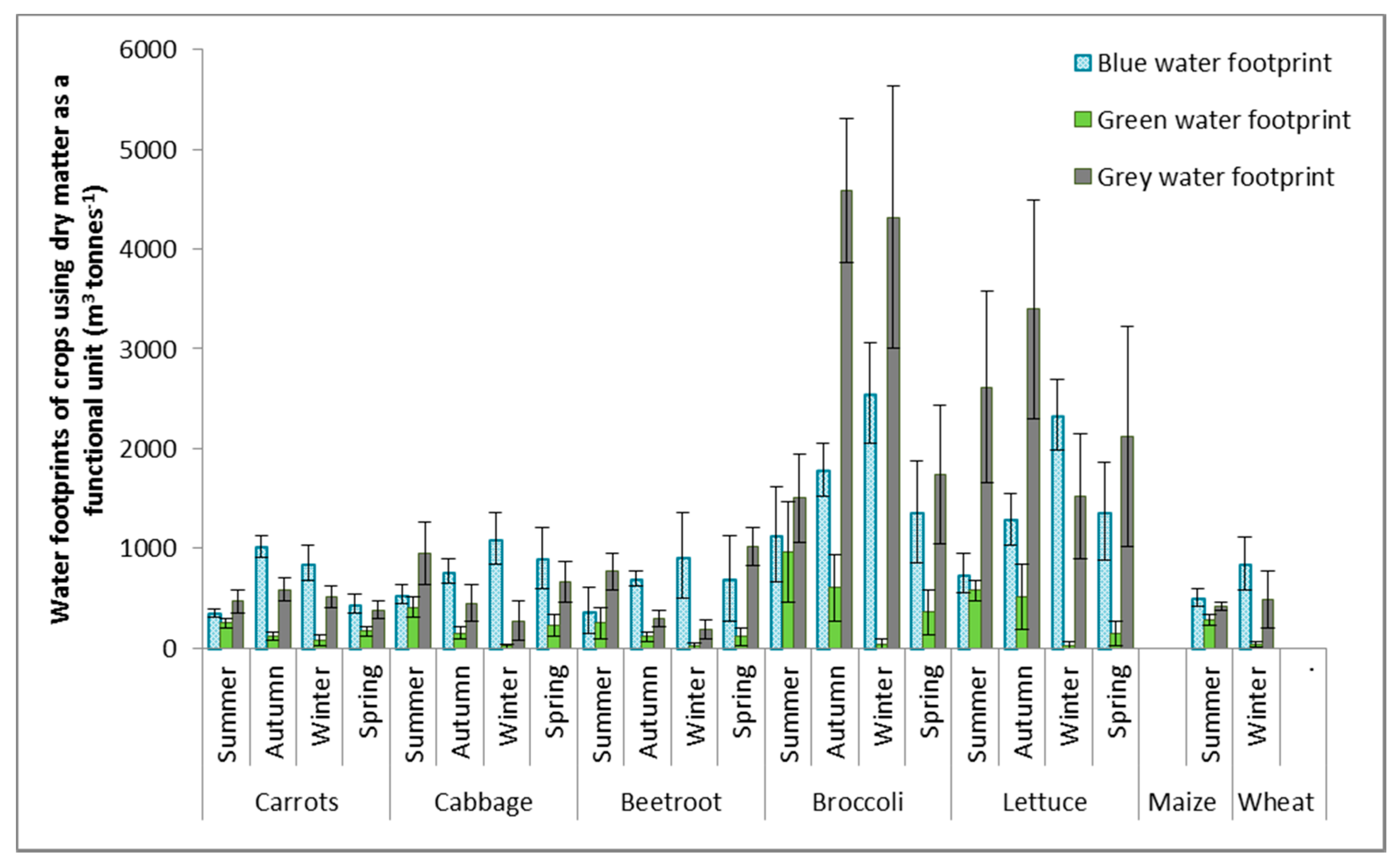
63] reported increased green WFs in high rainfall parts of the High Plains Aquifer (HPA) and increased blue WFs in parts of the HPA with low rainfall and higher temperatures. By calculating average WFs for crops from 1996 to 2005, Mekonnen and Hoekstra [
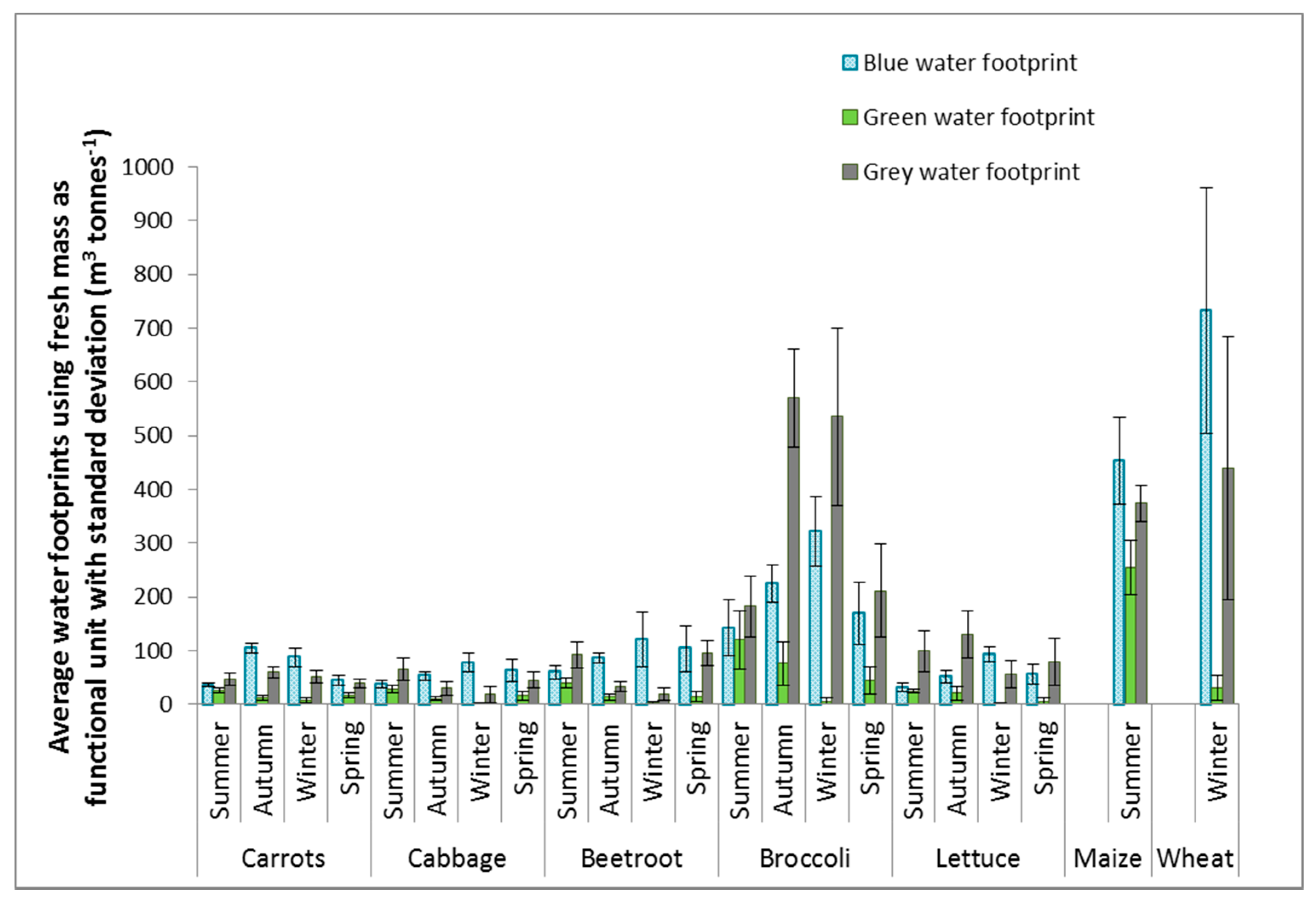
13] recognised the inter-annual variation in WFs of crops. Our results show that it is also important to interpret WFs with specific reference to the growing season, especially for short season crops with a range of planting date options. High inter-annual variation for this case study was illustrated by the WF high standard deviations of some crops during certain growing seasons, for example broccoli in summer with an average blue plus green WF of 262 m3·tonnes−1 and a standard deviation of 105 m3·tonnes−1.
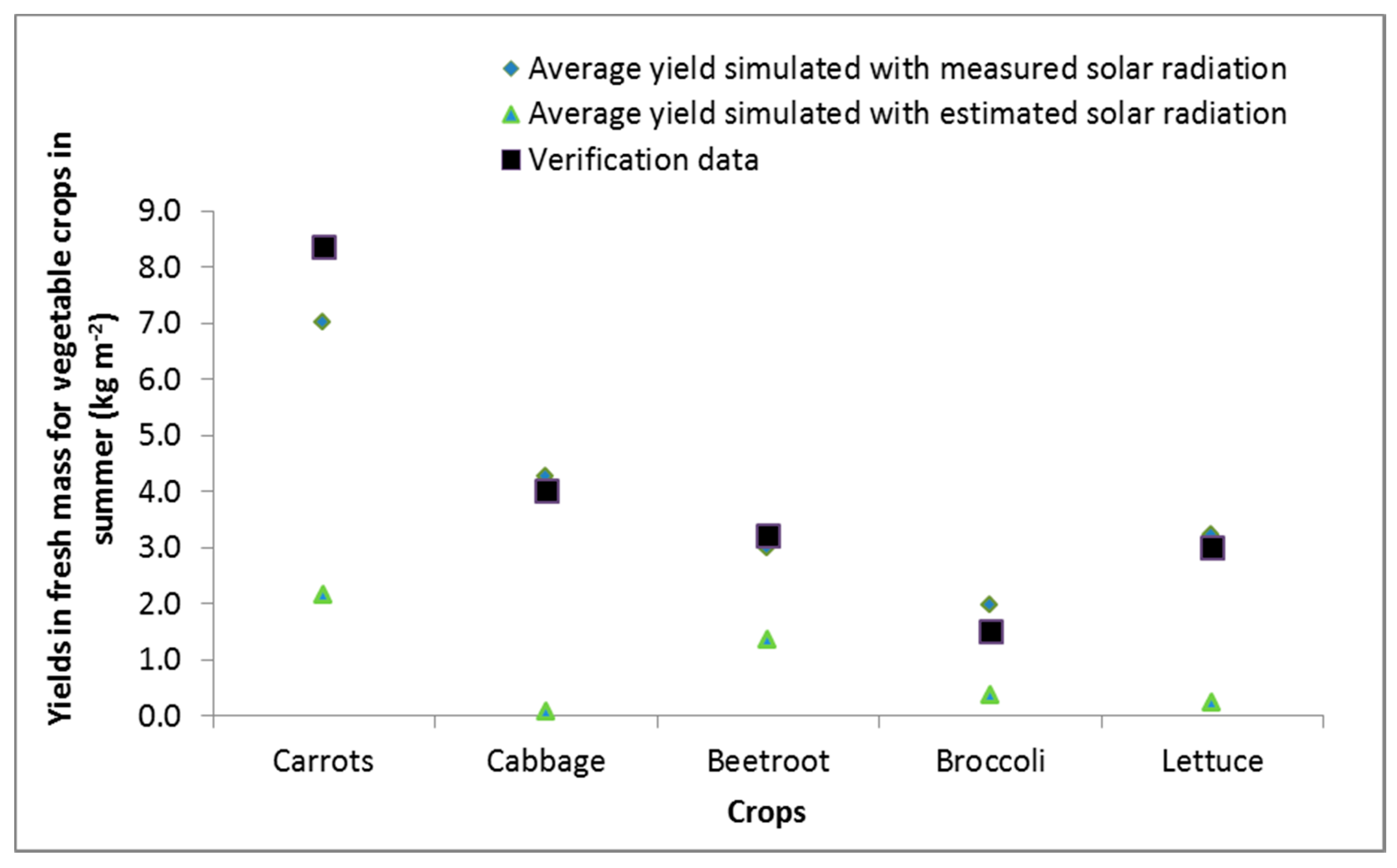
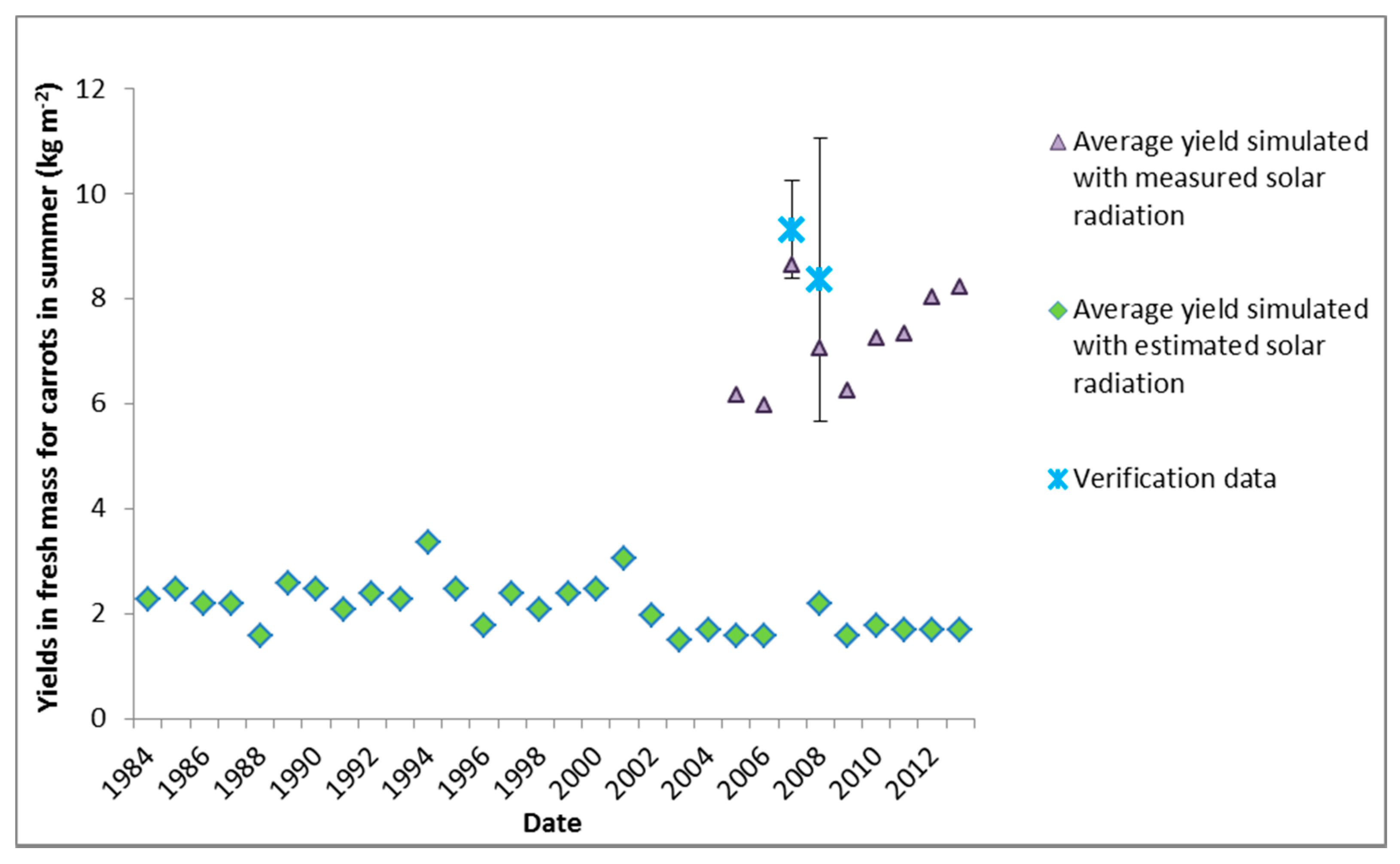
It should be widely recognised that WF estimates can be significantly influenced by the quality of data used to parameterise and run crop models. We observed that daily ETo estimates can differ significantly when either measured or estimated solar radiation data is used for its calculation, so we recommend that consistent weather data be used from parameterisation (creating crop parameters) to model application (using crop parameters for model simulations to obtain outputs). This was observed particularly for solar radiation during summer and spring for our study region. Using estimated solar radiation data for crops planted in autumn and winter, however, resulted in smaller differences in ETo and yield estimates. Therefore, the consistency in weather data that is used could potentially have a significant impact on WF results. Zhuo et al. [65] obtained similar results with a sensitivity analysis of WFs of maize, soybeans, rice and wheat to errors in input variables. They found that WFs of these crops are particularly sensitive to variations in ETo. The comparison between WFs calculated using more generic data from Mekonnen and Hoekstra [13] as given in Table 5 not only highlights the importance of reporting WFs for a specific season, it also highlights the need to use local data where possible, for example to parameterise a specific crop. All WFs reported by Mekonnen and Hoekstra [13] had a higher green and lower blue WF, while WFs generated using more detailed local data had a higher blue and lower green WF. This is due to the study area being located in the dry summer rainfall high central plateau of South Africa. The study area is considered to represent other areas in South Africa and around the world with similar climatic conditions.
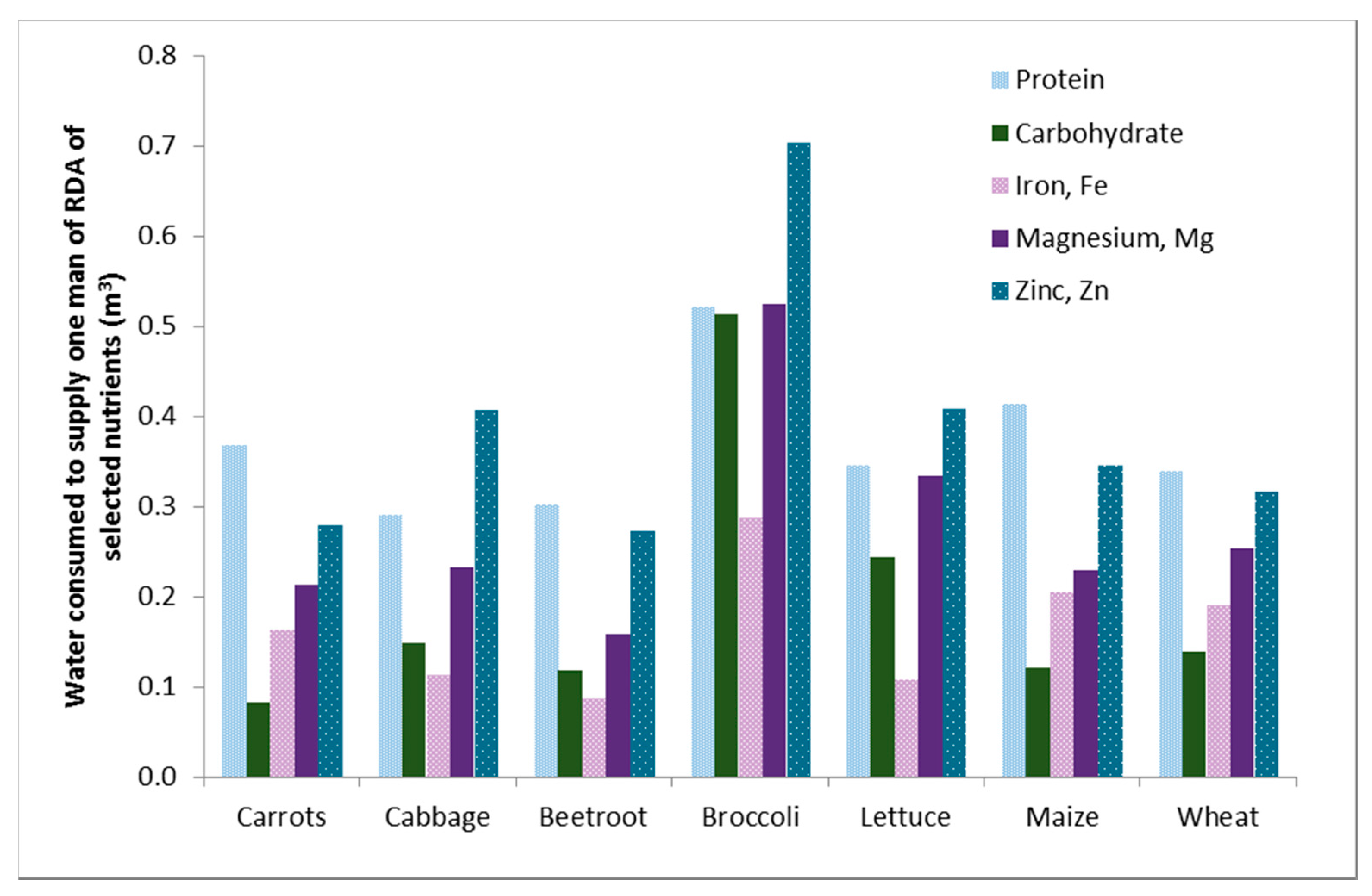
The functional unit used to calculate WFs has a significant impact on WF metrics. Grains with low moisture content, such as maize and wheat, will have a disproportionately high WF compared to vegetables when using fresh mass yields. Depending on the objective of the study, different functional units for various crops can be used to reveal which crops will be more efficient in producing important nutrients per volume of water. Assessing WFs in terms of other functional units such as economic gain and job creation is recommended for future research, because these alternative assessments can provide important information on how to allocate limited water supplies to achieve various objectives.
The high WF of broccoli due to the low relative yield of the harvestable portion that is produced by the crop presents a complexity and potential drawback in the application of the WF information, because the rest of the plant is often used for composting or animal feed. It can be argued that the beneficial use of the rest of the plant increases the total yield, and should be reflected in the WF. This could also be the case for many other crops. Compost will be incorporated into and increase the yield of the next crop and benefit soil health and the long term sustainability of the system. Therefore, composting the non-edible part of the previous crop will potentially reduce the WF of the next crop. It can also be argued from a different point of view if one uses compost to reduce the need for fertilisers. Production of fertilisers will have a certain WF and the compost will reduce the WF of the crop by reducing the need for fertiliser and the water required to produce the fertiliser. The blue, green and grey WF of fertilisers has not yet been addressed. Composting can also reduce the grey water footprint, because the use of organic N will potentially reduce the need for inorganic N and create N use efficiency.
The grey WF is a way of reporting impacts on water quality, which is a very important aspect of water resource management. The concept has, however, often been criticized for being too simplistic [66,67,68]. In a crop production context, water pollution is an especially complex issue. There are uncertainties in the determination of the N load leaching into the aquifer, because the fate of N is not well understood. Phosphates, salts, sediments and pesticides are also pollutants associated with agriculture, and need to be taken into account when addressing water quality. Therefore, it is not completely effective to assess the water quality impacts based on one pollutant. Similar to the WFs based on different nutrients, the grey water footprint can be calculated for various pollutants and the highest WF can be used as the total. The intensive use of fertilisers and the vulnerability of the aquifer to pollutants, as indicated by Witthueser, et al. [69], suggested that some impact could be expected on the water quality due to cultivation of crops. However, water quality analyses of the underlying groundwater indicated very good quality water, despite the intensive farming that has occurred over the past few decades. It is clear that the process of water pollution and pollutants leaching into the groundwater in the Steenkoppies Aquifer is still not well understood. A simplified method such as the grey WF does not provide the necessary information to improve water quality management of an aquifer. The use of grey WFs also becomes complex in a crop production context in cases where compost is used. Future research needs to address the potential benefits of composting crop residues in terms of the grey WF.
Despite the complexities addressed in this paper, WFs potentially provide useful information for water resource planning at the farm level. Knowing the blue and green WFs of crops in different seasons and the volume of water allocated, farmers can make better decisions about which crops to plant and when.

5. Conclusions

If water becomes scarce, farmers and water resource managers will have to ask the question of what they want to achieve with the available water. WF information can inform farmers to plant less water intensive crops or water resource managers to restrict certain crops during dry years or months. However, the method becomes complicated in a crop production context, because of inter-seasonal and inter-annual variations in WFs, the importance of local crop parameters and the requirement for comprehensive weather data. Crops, such as broccoli, with a low harvestable index will have a high WF, not representing how the residues of the plant are potentially used for other beneficial uses such as composting and animal feed. Water footprints that are calculated using fresh mass as a functional unit results in high WFs of crops with low water contents, such as maize and wheat, as compared to crops with high water contents, such as the vegetable crops. If WFs are calculated using dry matter, the high WFs of maize and wheat become more similar to the WFs of the vegetables. Using alternative functional units, such as nutritional content, potentially provides more meaningful information, which allows managers to make more informed decisions about water management and allocation. The current grey WF did not explain why the N concentration of the groundwater is within domestic drinking water standards, despite decades of agricultural activities on the Steenkoppies Aquifer. This could be due to an underestimation of the N load that reaches the aquifer or a big lag in the system. The following opportunities for future research have been identified:
  • Incorporate beneficial uses of crop residues in the WF.
  • Calculate WFs using other functional units, such as economic gain and job creation.
  • Improve the understanding of the fate of N for grey WF calculations.
  • Improve the understanding of how initial soil water content at planting could impact the blue versus green WF.
  • Determine how significant the variation in WFs is between different crop cultivars.

Acknowledgments

This study was funded by the Water Research Commission (WRC) of South Africa. The first author, Betsie le Roux, conducted this study as part of her Ph.D. studies, for which she received funding from the WRC and the National Research Foundation (NRF) of South Africa.

Author Contributions

The first author, Betsie le Roux, conducted this research and wrote the paper as part of her Ph.D. studies; Michael van der Laan supervised the research; Teunis Vahrmeijer contributed to the research in gathering data and developing the crop parameters for modeling; John G. Annandale and Keith L. Bristow are specialists in the field and acted as reviewers and mentors.

Conflicts of Interest

The authors declare no conflict of interest.

Abbreviations

The following abbreviations are used in this manuscript:
ETEvapotranspiration
EToReference Evapotranspiration
FAOFood and Agriculture Organization of the United States
HPAHigh Plains Aquifer
NNitrogen
PPhosphorus
SWBSoil Water Balance crop water use model
WFWater Footprint
WFNWater Footprint Network

References

  1. Department of Water Affairs. National Water Resource Strategy; Department of Water Affairs: Pretoria, South Africa, 2013.
  2. Backeberg, G.R.; Reinders, F.B. Institutional reform and modernisation of irrigation systems in South Africa. In Proceedings of the 5th Asian Regional Conference of ICID, New Delhi, India, 6–11 December 2009.
  3. South Africa Yearbook 2014/15; Government Communication and Information System (GCIS): Pretoria, South Africa, 2015.
  4. Nieuwoudt, W.L.; Backeberg, G.R.; Du Plessis, H.M. The value of water in the south african economy: Some implications. Agrekon 2004, 43, 162–183. [Google Scholar] [CrossRef]
  5. De Jager, E. South Africa annual Total Rainfall General Information; South African Weather Services: Pretoria, South Africa, 2016.
  6. Crop Estimates Committee. Preliminary Area Planted and Preliminary Production Forecast—Summer Crops; Department of Agriculture, Forestry and Fisheries (DAFF): Pretoria, South Africa, 2016.
  7. Nditwani, T.; Basson, T.; Rossouw, J. Water Reconciliation Strategy for the Crocodile (West) River catchment. Civ. Eng. 2009, 17, 14–18. [Google Scholar]
  8. Hoekstra, A.Y.; Chapagain, A.K.; Aldaya, M.M.; Mekonnen, M.M. The Water Footprint Assessment Manual: Setting the Global Standard; Routledge: London, UK, 2011. [Google Scholar]
  9. Deurer, M.; Green, S.R.; Clothier, B.E.; Mowat, A. Can product water footprints indicate the hydrological impact of primary production?—A case study of New Zealand kiwifruit. J. Hydrol. 2011, 408, 246–256. [Google Scholar] [CrossRef]
  10. Postel, S. Pillar of Sand: Can the Irrigation Miracle Last? W.W. Norton & Company United States of America: New York, NY, USA, 1999. [Google Scholar]
  11. Mostafa, M.E. Water in arid agriculture: Salinity and waterlogging in the near-east region. Ambio 1977, 6, 36–39. [Google Scholar]
  12. Zilberman, D.; Chakravorty, U.; Shah, F. Efficient management of water in agriculture. In Decentralization and Coordination of Water Resource Management; Parker, D.D., Tsur, Y., Eds.; Springer: Boston, MA, USA, 1997; pp. 221–246. [Google Scholar]
  13. Mekonnen, M.M.; Hoekstra, A.Y. The green, blue and grey water footprint of crops and derived crop products. Hydrol. Earth Syst. Sci. 2011, 15, 1577–1600. [Google Scholar] [CrossRef]
  14. Nyambo, P.; Wakindiki, I.I. Water footprint of growing vegetables in selected smallholder irrigation schemes in South Africa. Water SA 2015, 41, 571–578. [Google Scholar] [CrossRef]
  15. Scheepers, M.E.; Jordaan, H. Assessing the blue and green water footprint of lucerne for milk production in South Africa. Sustainability 2016, 8, 49. [Google Scholar] [CrossRef]
  16. Van der Laan, M.; Jumman, A.; Perret, S. Environmental benefits of improved water and nitrogen management in irrigated sugar cane: A combined crop modelling and life cycle assessment approach. Irrig. Drain. 2015, 64, 241–252. [Google Scholar] [CrossRef]
  17. Jongschaap, R.; Blesgraaf, R.; Bogaard, T.; Van Loo, E.; Savenije, H. The water footprint of bioenergy from Jatropha curcas l. Proc. Natl. Acad. Sci. USA 2009, 106, E92. [Google Scholar] [CrossRef] [PubMed]
  18. SABMiller; WWF. Water Footprinting: Identifying & Addressing Water Risks in the Value Chain; SABMiller: Woking, UK; WWF: Woking, UK, 2009. [Google Scholar]
  19. Pegasys. Water Footprint Analysis for the Breede Catchment, South Africa Draft Report; Breede Overberg Catchment Management Agency: Cape Town, South Africa, 2012. [Google Scholar]
  20. Pahlow, M.; Snowball, J.; Fraser, G. Water footprint assessment to inform water management and policy making in South Africa. Water SA 2015, 41, 300–313. [Google Scholar] [CrossRef]
  21. Ranchod, N.; Sheridan, C.M.; Pint, N.; Slatter, K.; Harding, K.G. Assessing the blue-water footprint of an opencast platinum mine in South Africa. Water SA 2015, 41, 287–293. [Google Scholar] [CrossRef]
  22. Department of Water and Sanitation. Long Term Flow Data for the Maloneys’ Eye. Available online: https://www.dwa.gov.za/Hydrology/hymain.aspx (accessed on 1 June 2014).
  23. Vahrmeijer, J.; Annandale, J.; Bristow, K.; Steyn, J.; Holland, M. Drought as a catalyst for change: A case study of the steenkoppies dolomitic aquifer. In Drought in Arid and Semi-Arid Regions; Springer: New York, NY, USA, 2013; pp. 251–268. [Google Scholar]
  24. Water Research Commission. WRC Knowledge Review for 2013/14; Water Research Commission: Pretoria, South Africa, 2014. [Google Scholar]
  25. AgroClimatology Staff. ARC-ISCW Climate Information System; ARC-Institute for Soil, Climate and Water: Pretoria, South Africa, 2014. [Google Scholar]
  26. Ridoutt, B.G.; Pfister, S. A revised approach to water footprinting to make transparent the impacts of consumption and production on global freshwater scarcity. Glob. Environ. Chang. 2010, 20, 113–120. [Google Scholar] [CrossRef]
  27. Hoekstra, A.Y.; Chapagain, A.K. Globalization of Water: Sharing the Planet’s Freshwater Resources; John Wiley & Sons: New York, NY, USA, 2011. [Google Scholar]
  28. Annandale, J.; Benade, N.; Jovanovic, N.; Steyn, J.; Du Sautoy, N. Facilitating Irrigation Scheduling by Means of the Soil Water Balance Model; Water Research Commission Report. No. 753/1/99; Water Research Commission: Pretoria, South Africa, 1999. [Google Scholar]
  29. Allen, R.G.; Pereira, L.S.; Raes, D.; Smith, M. Crop Evapotranspiration-Guidelines for Computing Crop Water Requirements-FAO Irrigation and Drainage Paper 56; FAO: Rome, Italy, 1998. [Google Scholar]
  30. Annandale, J.; Campbell, G.; Olivier, F.; Jovanovic, N. Predicting crop water uptake under full and deficit irrigation: An example using pea (Pisum sativum L. Cv. Puget). Irrig. Sci. 2000, 19, 65–72. [Google Scholar] [CrossRef]
  31. Annandale, J.G.; Stirzaker, R.J.; Singels, A.; Van der Laan, M.; Laker, M.C. Irrigation scheduling research: South african experiences and future prospects. Water SA 2011, 37, 751–763. [Google Scholar] [CrossRef]
  32. Jovanovic, N.; Annandale, J. Crop growth model parameters of 19 summer vegetable cultivars for use in mechanistic irrigation scheduling models. Water SA 2000, 26, 67–76. [Google Scholar]
  33. Jovanovic, N.; Annandale, J.; Mhlauli, N. Field water balance and swb parameter determination of six winter vegetable species. Water SA 1999, 25, 191–196. [Google Scholar]
  34. Vahrmeijer, J. Improved Management of Groundwater in Irrigated Catchments under Stress. Ph.D. Thesis, University of Pretoria, Pretoria, South Africa, 2016. [Google Scholar]
  35. Jovanovic, N.; Ehlers, L.; Bennie, A.; Du Preez, C.; Annandale, J. Modelling the contribution of root accessible water tables towards crop water requirements. S. Afr. J. Plant Soil 2004, 21, 171–181. [Google Scholar] [CrossRef]
  36. Nagar, B.; Datta, M.; Khakhar, M. Eutrophication and recovery in experimental lakes: Implications for lake management. Science 1974, 184, 897–899. [Google Scholar]
  37. Schindler, D.W. Recent advances in the understanding and management of eutrophication. Limnol. Oceanogr. 2006, 51, 356–363. [Google Scholar] [CrossRef]
  38. Schindler, D.; Fee, E. Experimental lakes area: Whole-lake experiments in eutrophication. J. Fish. Res. Board Can. 1974, 31, 937–953. [Google Scholar] [CrossRef]
  39. Conley, D.J.; Paerl, H.W.; Howarth, R.W.; Boesch, D.F.; Seitzinger, S.P.; Karl, E.; Lancelot, C.; Gene, E. Controlling eutrophication: Nitrogen and phosphorus. Science 2009, 123, 1014–1015. [Google Scholar] [CrossRef] [PubMed]
  40. Walton, G. Survey of literature relating to infant methemoglobinemia due to nitrate-contaminated water. Am. J. Public Health Nations Health 1951, 41, 986–996. [Google Scholar] [CrossRef] [PubMed]
  41. Smolders, A.J.; Lucassen, E.C.; Bobbink, R.; Roelofs, J.G.; Lamers, L.P. How nitrate leaching from agricultural lands provokes phosphate eutrophication in groundwater fed wetlands: The sulphur bridge. Biogeochemistry 2010, 98, 1–7. [Google Scholar] [CrossRef]
  42. Sims, J.T.; Simard, R.R.; Joern, B.C. Phosphorus loss in agricultural drainage: Historical perspective and current research. J. Environ. Qual. 1998, 27, 277–293. [Google Scholar] [CrossRef]
  43. Gleeson, T.; Alley, W.M.; Allen, D.M.; Sophocleous, M.A.; Zhou, Y.; Taniguchi, M.; VanderSteen, J. Towards sustainable groundwater use: Setting long-term goals, backcasting, and managing adaptively. Ground Water 2012, 50, 19–26. [Google Scholar] [CrossRef] [PubMed]
  44. Chapagain, A.; Hoekstra, A. The blue, green and grey water footprint of rice from production and consumption perspectives. Ecol. Econ. 2011, 70, 749–758. [Google Scholar] [CrossRef]
  45. Mekonnen, M.M.; Hoekstra, A.Y. A global assessment of the water footprint of farm animal products. Ecosystems 2012, 15, 401–415. [Google Scholar] [CrossRef]
  46. Mekonnen, M.; Hoekstra, A. A global and high-resolution assessment of the green, blue and grey water footprint of wheat. Hydrol. Earth Syst. Sci. 2010, 14, 1259–1276. [Google Scholar] [CrossRef] [Green Version]
  47. Department of Water Affairs and Forestry (DWAF). General and Special Limits Applicable to Discharge of Wastewater into a Water Resource; Government Gazette 20526; DWAF: Pretoria, South Africa, 1999.
  48. Department of Water Affairs (DWA). Water Quality Data for the Maloney’s Eye; Monitoring Point ID 90163; DWA: Pretoria, South Africa, 2014.
  49. Franke, N.A.; Boyacioglu, H.; Hoekstra, A.Y. Grey Water Footprint Accounting: Tier 1 Supporting Guidelines; Value of Water Research Report Series No. 65; UNESCO-IHE: Delft, The Netherlands, 2013. [Google Scholar]
  50. Van Suid Afrika, M. Bemestingshandleiding, 7th ed.; FSSA-MVSA: Pretoria, South Africa, 2007. [Google Scholar]
  51. Petek, M.; Custic, M.H.; Nina, T.; Slunjski, S.; Lepomir, C.; Pavlovic, I.; Karazija, T.; Lazarevic, B.; Cvetkovi, S. Nitrogen and crude proteins in beetroot (Beta vulgaris var. conditiva) under different fertilization treatments. Not. Bot. Horti Agrobot. 2012, 40, 215–219. [Google Scholar]
  52. Sorensen, J. Nitrogen effects on vegetable crop production and chemical composition. In Proceedings of the International Workshop on Ecological Aspects of Vegetable Fertilization in Integrated Crop Production, Warwick, UK, 27–31 July 1998; pp. 41–50.
  53. Australian and New Zealand Environment and Conservation Council (ANZECC); Agriculture and Resource Management Council of Australia and New Zealand (ARMCANZ). Australian and New Zealand Guidelines for Fresh and Marine Water Quality; ANZECC: Canberra, Australia; ARMCANZ: Canberra, Australia, 2000.
  54. Alexandrova, P.; Donov, D. Nitrogen content and its uptake by maize as influenced by some meteorological elements and fertilization. Int. Agrophys. 2003, 17, 41–46. [Google Scholar]
  55. Mossé, J.; Huet, J.; Baudet, J. The amino acid composition of wheat grain as a function of nitrogen content. J. Cereal Sci. 1985, 3, 115–130. [Google Scholar] [CrossRef]
  56. Allan, J.A. Virtual water: A strategic resource global solutions to regional deficits. Ground Water 1998, 36, 545–546. [Google Scholar] [CrossRef]
  57. Rebitzer, G.; Ekvall, T.; Frischknecht, R.; Hunkeler, D.; Norris, G.; Rydberg, T.; Schmidt, W.-P.; Suh, S.; Weidema, B.P.; Pennington, D.W. Life cycle assessment: Part 1: Framework, goal and scope definition, inventory analysis, and applications. Environ. Int. 2004, 30, 701–720. [Google Scholar] [CrossRef] [PubMed]
  58. Schau, E.M.; Fet, A.M. LCA studies of food products as background for environmental product declarations. Int. J. Life Cycle Assess. 2008, 13, 255–264. [Google Scholar] [CrossRef]
  59. Ingwersen, W.W. Life cycle assessment of fresh pineapple from costa rica. J. Clean. Prod. 2012, 35, 152–163. [Google Scholar] [CrossRef]
  60. United States Department of Agriculture. National Nutrient Database for Standard Reference. Available online: http://ndb.nal.usda.gov/ (accessed on 2 June 2015).
  61. Mahan, L.K.; Escott-Stump, S. Krause’s Food, Nutrition, & Diet Therapy, 11th ed.; Elsevier: New York, NY, USA, 2004. [Google Scholar]
  62. Wiegmans, F.; Holland, M.; Janse van Rensburg, H. Groundwater Resource Directed Measures for Maloney’s Eye Catchment; Report No. 14/14/5/2; Water Research Commission Report No. K8/970; Water Research Commission: Pretoria, South Africa, 2013. [Google Scholar]
  63. Multsch, S.; Pahlow, M.; Ellensohn, J.; Michalik, T.; Frede, H.-G.; Breuer, L. A hotspot analysis of water footprints and groundwater decline in the high plains aquifer region, USA. Reg. Environ. Chang. 2016. [Google Scholar] [CrossRef]
  64. Sun, S.; Wu, P.; Wang, Y.; Zhao, X. Temporal variability of water footprint for maize production: The case of beijing from 1978 to 2008. Water Resour. Manag. 2013, 27, 2447–2463. [Google Scholar] [CrossRef]
  65. Zhuo, L.; Mekonnen, M.; Hoekstra, A. Sensitivity and uncertainty in crop water footprint accounting: A case study for the yellow river basin. Hydrol. Earth Syst. Sci. 2014, 18, 2219–2234. [Google Scholar] [CrossRef]
  66. Ridoutt, B.G.; Pfister, S. A new water footprint calculation method integrating consumptive and degradative water use into a single stand-alone weighted indicator. Int. J. Life Cycle Assess. 2013, 18, 204–207. [Google Scholar] [CrossRef]
  67. Wichelns, D. Assessing water footprints will not be helpful in improving water management or ensuring food security. Int. J. Water Resour. Dev. 2011, 27, 607–619. [Google Scholar] [CrossRef]
  68. Perry, C. Water footprints: Path to enlightenment, or false trail? Agric. Water Manag. 2014, 134, 119–125. [Google Scholar] [CrossRef]
  69. Witthueser, K.; Leyland, R.; Holland, M. Vulnerability of dolomite aquifers in South Africa. In Sustainable Groundwater Resources in Africa: Water Supply and Sanitation Environment; Xu, Y., Braune, E., Eds.; CRC Press: Roggebaai, South Africa, 2009; pp. 119–131. [Google Scholar]
Figure 1. Soil Water Balance (SWB) model simulated yields versus actual yields of carrots grown in summer indicating the influence of using estimated versus measured solar radiation data on simulated yield results with standard deviations shown as error bars.
Water 08 00473 g001
Figure 2. Soil Water Balance (SWB) model results for simulated and measured yield of carrots, cabbage, beetroot, broccoli and lettuce grown in summer with measured and estimated solar radiation.
Water 08 00473 g002
Figure 3. Correlation between verification yield data and yields simulated with the Soil Water Balance model using measured solar radiation data for carrots, cabbage, beetroot, broccoli and lettuce grown in summer.
Water 08 00473 g003
Figure 4. Average of 10 years’ simulated seasonal irrigation (2004–2013) with standard deviations (shown as error bars) of vegetable crops in the different growing seasons compared to measured irrigation verification data from farms on the Steenkoppies Aquifer.
Water 08 00473 g004
Figure 5. Average of 10 years’ simulated seasonal yields (2004–2013) with standard deviations (shown as error bars) of vegetable crops for the different growing seasons compared to measured fresh mass yield data from the farms on the Steenkoppies Aquifer.
Water 08 00473 g005
Figure 6. Average of 10 years’ blue and green water footprints (2004–2013) with standard deviations (shown as error bars) of vegetable and grain crops in the different growing seasons on the Steenkoppies Aquifer using fresh mass as a functional unit.
Water 08 00473 g006
Figure 7. Average of 10 years’ blue and green water footprints (2004–2013) with standard deviations (shown as error bars) of vegetable and grain crops in the different growing seasons on the Steenkoppies Aquifer using dry matter as a functional unit.
Water 08 00473 g007
Figure 8. Blue plus green water footprint to supply a man (aged 31–50) with their Recommended Dietary Allowance (RDA) [61] in terms of selected nutrients.
Water 08 00473 g008
Table 1. Locally produced crop parameters used in the Soil Water Balance model to simulate the data required for WF calculations.
ParametersCarrotsCabbageBeetrootBroccoliLettuceMaizeWheat
Summer & SpringAutumn & WinterSummer & SpringAutumn & WinterSummerSpringAutumn & WinterSummer & SpringAutumn & WinterAll SeasonsSummerWinter
Extinction Coefficient0.760.760.780.620.640.640.640.770.810.920.560.55
Dry-Matter-Water Ratio (Pa)889677767944
Conversion Efficiency (kg·MJ−1)0.000870.000870.000940.000940.00120.00120.00120.0010.0010.00090.00120.0017
Base temperature (°C)7.27.24.424.44.44.4007.2104
Temperature Optimal Light (°C)151515101515151510152515
Cut Off Temperature (°C)23.923.923.923.923.923.923.923.923.923.93025
Emergence Day Degrees (°C)1031031305064646412395715050
Flowering Day Degrees (°C)2002008007502002005001100650175900750
Maturity Day Degrees (°C)14501300130014451300100013561700120052917001500
Transition Day Degrees (°C)12381238400500700700700500120047510400
Maximum Leaf Age145013001300144513001000135617001200529900900
Max Height (m)0.40.40.40.40.40.40.40.50.40.32.21
Maximum Root Depth (m)0.60.60.60.60.60.60.60.60.60.60.60.4
Stem to Grain Translation0.50.50.050.050.50.50.50.50.50.010.050.01
Canopy Storage (mm)111111111111
Minimum Leaf Water Potential (kPa)−1500−1500−1500−1500−1500−1500−1500−1500−1500−1500−2000−1500
Maximum Transpiration (mm·day−1)999999999999
Specific Leaf Area (m2·kg−1)17.917.9119.513131310.59.5201512
Leaf Stem Partition (m2·kg−1)3.083.081.550.563.023.023.021.541.546.330.81.2
Total Dry Mass at Emergence or Transplanting (kg·m−2)0.00050.00050.0050.010.0030.0030.0030.0010.0070.00080.00190.0019
Root Fraction0.10.10.10.10.20.20.20.20.10.20.010.02
Root Growth Rate222244422247
Stress Index0.950.950.950.950.950.950.950.950.950.950.950.95
Table 2. Nitrogen application rates and nitrogen content of all selected crops used to determine surplus nitrogen applied.
CropsApplication (kg·N·ha−1)N content of Fresh Mass (%)
Beetroot1400.2% [51]
Carrots1900.12% [52]
Cabbage1900.2% [52]
Broccoli1900.4% [52]
Lettuce1300.19% [53]
Maize2200.9% [54]
Wheat2401.5% [55]
Table 3. Percentage crop dry matter used to convert Soil Water Balance model dry matter results to fresh mass.
CropsPercentage Dry Matter
Carrots10% 1
Cabbage7% 1
Beetroot13% 2
Broccoli13% 1
Lettuce4% 2
Maize90% 2
Wheat87% 2
Notes: 1 Assumed constant percentage; 2 obtained from United States Department of Agriculture [60].
Table 4. Recommended Dietary Allowance (RDA) of selected nutrients required daily by men aged 31–50 years [61].
NutrientRDA of a Man Aged 31 to 50
Proteins56 g
Carbohydrates130 g
Iron8 mg
Magnesium420 mg
Zinc11 mg
Table 5. Blue, green and grey water footprints using fresh mass as a functional unit for cultivating vegetable crops, maize and wheat on the Steenkoppies Aquifer compared to outcomes from the literature.
CropMonthAverage Seasonal WF of Crop (m3·Tonnes−1)WFs (m3·Tonnes−1) Reported in the Literature [13]Percentage Difference between Local and Published Blue + Green WFs
BlueGreenBlue + GreenGreyBlueGreenBlue + GreenGrey
CarrotsSummer362561482810613461120%
Autumn104121166015%
Winter887955241%
Spring45176239116%
CabbageSummer382966652618120773212%
Autumn53116430224%
Winter7717918163%
Spring63167945162%
BeetrootSummer6040100922682108258%
Autumn8714101337%
Winter121312419−13%
Spring1041511895−9%
BroccoliSummer1421202621822118921075−20%
Autumn22576301570−30%
Winter3225327535−36%
Spring17044214212−2%
LettuceSummer312456992813316177256%
Autumn512071130169%
Winter9319355108%
Spring5666279212%
MaizeSummer45225470737381947102819445%
WheatWinter7323176243934212771619207120%

