
Spatial Quantification of Non-Point Source Pollution in a Meso-Scale Catchment for an Assessment of Buffer Zones Efficiency

 , , ,
, , ,
Abstract
: The objective of this paper was to spatially quantify diffuse pollution sources and estimate the potential efficiency of applying riparian buffer zones as a conservation practice for mitigating chemical pollutant losses. This study was conducted using a semi-distributed Soil and Water Assessment Tool (SWAT) model that underwent extensive calibration and validation in the Sulejów Reservoir catchment (SRC), which occupies 4900 km2 in central Poland. The model was calibrated and validated against daily discharges (10 gauges), NO3–N and TP loads (7 gauges). Overall, the model generally performed well during the calibration period but not during the validation period for simulating discharge and loading of NO3–N and TP. Diffuse agricultural sources appeared to be the main contributors to the elevated NO3–N and TP loads in the streams. The existing, default representation of buffer zones in SWAT uses a VFS sub-model that only affects the contaminants present in surface runoff. The results of an extensive monitoring program carried out in 2011–2013 in the SRC suggest that buffer zones are highly efficient for reducing NO3–N and TP concentrations in shallow groundwater. On average, reductions of 56% and 76% were observed, respectively. An improved simulation of buffer zones in SWAT was achieved through empirical upscaling of the measurement results. The mean values of the sub-basin level reductions are 0.16 kg NO3/ha (5.9%) and 0.03 kg TP/ha (19.4%). The buffer zones simulated using this approach contributed 24% for NO3–N and 54% for TP to the total achieved mean reduction at the sub-basin level. This result suggests that additional measures are needed to achieve acceptable water quality status in all water bodies of the SRC, despite the fact that the buffer zones have a high potential for reducing contaminant emissions.1. Introduction
1.1. Water Management Context
Fulfilling the requirements of the European Water Framework Directive [1] and the Nitrates Directive [2] by reducing pollution emissions to water ecosystems remains a major challenge faced in water management. Particularly, the main issue is the reduction of non-point pollution that originates from agricultural land. The contributions of agriculture to the pool of nitrogen and phosphorus compounds in water ecosystems are high.
In Poland, the large share of farmland consisting of highly fragmented arable land and strongly dispersed developments has resulted in major pressure from pollution emission sources, including (1) pressure from agriculture related to the use of inappropriate farming practices (transport of organic and mineral nitrogen and phosphorus compounds from fertilizers to the environment) and (2) pressure from scattered households that are not connected to sewage systems.
Thus, the development of N and P reduction strategies is a major task for water authorities throughout Europe. One example of activities that are undertaken to achieve sustainable water management goals in agricultural catchments is the EU-funded EKOROB project (Ecotones for reducing diffuse pollution). The main objective of this project is to develop an Action Plan for reductions of diffuse pollution in the Pilica River catchment (Poland) and will help achieve a good ecological status for the water in the Sulejów Reservoir, particularly by reducing eutrophication and decreasing the frequency and intensity of cyanobacterial blooms.
The Action Plan is based on the ecohydrology concept [3–5], which assumes that the basis for integrated river basin management is the quantification of catchment-scale processes that are part of the hydrological cycle. The concept of ecohydrology involves quantifying hydrological processes at the basin scale and the entire hydrological cycle to quantify ecological processes. This quantification includes the patterns of hydrological pulses along the river continuum and the identification of various human impacts on point and non-point sources of pollution [6]. Thus, this quantification should be the first step when developing regulatory processes for sustainable water use and ecosystem protection. Although many mathematical tools are available for this task, the Soil and Water Assessment Tool (SWAT) [7] is one of the most widely used and comprehensive tools.
1.2. The Use of SWAT for Quantifying Emission Sources
SWAT is a comprehensive hydrological/water quality model that is increasingly being used to address a wide variety of water resource problems across the globe [8]. Several studies have investigated the spatial variability and distribution of various pollutant emissions/losses in catchments of different sizes [9–12]. Niraula et al. [9] calibrated SWAT (and a less complex GWLF model) for a small catchment in Alabama and used it to identify Critical Source Areas (CSAs) for sediment, TN and TP based on the loadings per unit area (yield or emission or losses) at the sub-basin level. Another application of SWAT in a medium-sized Greek catchment resulted in similar findings, but with a finer level of Hydrological Response Units (HRUs) [10]. Wu and Chen [11] investigated the influences of point source and diffuse pollution on the water quality of a relatively large catchment in south China by using SWAT. These authors concluded that diffuse pollution overwhelmingly surpasses point source pollution for all constituents except TP. In addition, these authors identified CSAs at the HRU and sub-basin levels. Finally Wu and Liu [12] calibrated SWAT for a large catchment in Iowa and showed a relationship between the shares of agricultural areas with sediment and NO3–N emissions by using the calibrated model.
1.3. Riparian Buffer Zones and Their Modeling in SWAT
Riparian buffer zones (ecotones, vegetative filter strips) are an effective Best Management Practice (BMP) for buffering aquatic ecosystems against nutrient losses from the agricultural landscapes. Buffer zones are strips of permanent vegetation (including herbs, grasses, shrubs or trees) that are adjacent to aquatic ecosystems and used to maintain or improve water quality by trapping and removing various non-point source pollutants from overland and shallow sub-surface flow [13–16].
For pollutants transported in surface runoff, the process of sediment and nutrient trapping by buffer zones is reasonably well understood, particularly for grass filter strips (cf. review [17]). Reductions in the surface flow velocities due to the increased hydraulic roughness of the vegetation in the buffer enhanced particle deposition. Vought et al. [18] reported that a buffer strip with a width of 10 m can reduce phosphorus loads, which are typically bound to sediments, by as much as 95%. Buffer zone are effective for removing sediments and other suspended solids contained in surface runoff; however, soluble forms of nitrogen and phosphorus are not removed as effectively as sediments [19]. Results collected from 44 fields (row crops with slopes range from 1%–14%) showed that a 10-m buffer zone reduced the total suspended solids, soluble phosphorus and nitrate-nitrogen contents by 64%, 34% and 38%, respectively [20]. The efficiencies of narrow buffer zones (5–10 m) in Norway varied from 81%–91%, 60%–89% and 37%–81% for particles, total phosphorus and total nitrogen, respectively [21].
Buffer strips are normally less efficient for removing nitrate than orthophosphates from surface runoff. In contrast with orthophosphate, nitrogen is very labile and is not largely adsorbed within the soil [18]. However, the impacts of the sub-surface flow efficiency of the buffer zones on reducing nitrogen are well described in the literature and often reach a concentration reduction of 90% [17]. A meta-analysis of nitrogen removal in riparian buffers based on data from 65 individual riparian buffers from published studies indicated a mean removal effectiveness of 76.7% [22]. However, the efficiency of buffer zones for reducing phosphorus in shallow groundwater is not well documented, and some studies suggest that riparian zones are ineffective for removing dissolved phosphorus or could even release phosphorus to the water [23,24].
Buffer zones along small streams that are more exposed to pressure from agriculture are more efficient than buffer zones along larger rivers. A key factor for determining the efficiency of buffer zones is their continuity. Continuous and narrow riparian buffers are more efficient than wider and intermittent buffers [25]. Hence, an important issue for effective water management is the selection of priority areas that have the highest emissions of diffuse pollution. Next, concentrating measures, such as buffer zones, should be applied in these areas. Catchment-scale water quality modeling is one possible solution for quickly identifying priority areas.
Numerous examples are available regarding the application of SWAT for simulating the affects of buffer zones on diffuse pollution [26–29]. Older versions of SWAT used a very simplistic equation that was only based on filter width for calculating the HRU-level reduction rate of buffer zones. This equation was based on empirical data from the US regarding buffer strip efficiency [27,28]. Since then, SWAT has undergone certain modifications to address variable source areas within watersheds and vegetated buffers adjacent to streams [26,30]. The new VFS sub-model currently used in SWAT reduces the sediment, nitrate and phosphorus loading in streams as a function of estimated reductions in runoff. Hence, the new VFS sub-model only affects contaminants present in surface runoff and neglects nutrient trapping in shallow groundwater. As mentioned previously for nitrogen in sub-surface flow, buffer zones are very efficient measures [17]. However, little consensus has been reached for phosphorus [23,24]. This result suggests that the buffer zone efficiency is case-specific and depends on local conditions. Hence it is equally as important to apply existing models as it is to measure the efficiency of existing buffer zones in the field to gain more confidence regarding their behavior.
1.4. Objective
Two objectives of this paper are:
Spatial quantification of NO3–N and TP emissions from major pollution sources in a meso-scale catchment using SWAT.
Simulation of buffer zone effects on the mitigation of pollution losses when applied in Critical Source Areas through the combined use of the default SWAT VFS sub-model and local field monitoring data.
The term “meso-scale catchment” refers to catchments with an order of magnitude between 10 and 103 km2 [31]. A part of the Pilica catchment selected as the case study in this paper, a demonstration catchment of the EKOROB project, satisfies this condition.
2. Materials and Methods
2.1. Study Area
The study was conducted in the Sulejów Reservoir catchment (hereafter referred to as the SRC). Sulejów is a shallow and eutrophic artificial reservoir that was built in 1974 and is situated in the middle course of the Pilica River in central Poland. Two main tributaries supply water to the Sulejów Reservoir: the Pilica and Luciąża Rivers. At its full capacity, this reservoir covers an area of 22 km2, with a mean depth of 3.3 m and a volume of 75 × 106 m3. The Sulejów Reservoir was used as a drinking water reservoir for Łódź agglomeration until 2004 and is currently an important recreational site that has been extensively studied (cf. review [32]). Microcystis aeruginosa is the dominant species of bloom-forming cyanobacteria in the reservoir and produces microcystin-LR, microcystin-YR, and microcystin-RR [33–35].
The SWAT model is used in this study for the entire SRC area upstream of the dam, which occupies 4933 km2 (Figure 1). This area consists of the Pilica (contributing 79.8% of area) and the Luciąża (15.3%) River catchments and a direct reservoir sub-catchment with several smaller streams (4.9%). The elevation of the SRC varies from 154 m in the lowland areas in the north to 499 m in the highland areas in the south. The distribution of land cover in the SRC area is as follows: 44.4% arable land, 38.6% forest areas, 12.3% grasslands, and 4.7% urban areas (mainly low-density residential areas), with the remaining land occupied by other types of land cover (data according to Corine Land Cover 2006). The predominate soil types in this area are loamy sands and sands. The climate of this area is typical for central Poland, with a mean annual temperature of 7.5 °C and mean January and July temperatures of −4 °C and 18 °C, respectively. The mean annual precipitation is 600 mm. The highest amounts of precipitation occur in June/July, and the lowest amounts of precipitation occur in January. The flow regime is characterized by early spring snow-melt induced floods and summer low flows with occasional summer floods. The quantitative pressure on surface water resources is relatively low. The fish farming industry scattered around the catchment and the Cieszanowice Reservoir constructed in 1998 on the Luciąża River (volume of 7.3 × 10 m3 at full capacity) are the only considerable sources of flow alteration.
In contrast, multiple point and non-point pollution sources in the area result in elevated N and P loads flowing into the Sulejów Reservoir, which eventually contribute to toxic cyanobacterial blooms in its waters. These different sources will be described systematically in terms of SWAT model inputs in Sub-Section 2.4.
2.2. SWAT Model
2.2.1. General Features
SWAT is a physically based, semi-distributed, continuous-time model that simulates the movement of water, sediment, and nutrients on a catchment scale with a daily time step. The basic calculation unit, referred to as a “hydrological response unit” (HRU) is a combination of land use, soil, and slope overlay. Both water balance components, which is a driving force behind affect all processes that occur in a watershed, and water quality, output parameters are computed separately for each HRU. Water, nutrients and sediment leaving HRUs are aggregated at the sub-basin level and routed through the stream network to the main outlet to obtain the total flows and loadings for the river basin.
In this study, channel routing was modeled using a variable storage coefficient approach. The modified USDA Soil Conservation Service (SCS) curve number method for calculating surface runoff and the Penman-Monteith method for estimating potential evapotranspiration (PET) were selected. In the model, snow-melt estimations are based on the degree-day method. The SWAT adapted plant growth model, which is used to assess the removal of water and nutrients from the root zone, transpiration, and biomass/yield production, is based on EPIC [36]. The in-stream water quality component allows us to control nutrient transformations in the stream. The in-stream kinetics used in SWAT for nutrient routing are adapted from QUAL2E [37].
SWAT simulates the movement and transformation of several forms of nitrogen and phosphorus in the watershed. In the nitrogen cycle, the main processes are denitrification, nitrification, mineralization, plant uptake, decay, fertilization, and volatilization. In the phosphorus cycle, the main processes are mineralization, fertilization, decay, and plant uptake. The nutrient transport pathways from upland areas to stream networks correspond to the following hydrological transport pathways: surface runoff, lateral subsurface flow and groundwater flow. Additionally point source discharges of water and contaminants can be defined that are directly input into the water routed through the stream network.
From the point of view of modeling buffer zones in SWAT, it is important to note that HRUs are lumped and non-contiguous geographic units within each sub-basin. A SWAT model setup may consist of thousands of such units, and each of them may represent one field, a portion of a field, or, more likely, portions of many fields [38].
2.2.2. Runoff-Reduction-Based Buffer Zone Sub-Model
A key characteristic of the buffer zone sub-model implemented in SWAT is that it works at the HRU level and reduces the loads of sediment, nitrate and phosphorus that enter the stream as a function of estimated reductions in runoff. Hence, the sub-model only affects contaminants that are present in surface runoff and neglects the potential affects of buffer zones on shallow groundwater. This sub-model was developed and evaluated using measured data derived from the literature and included data that were collected using differing experimental protocols and under conditions with different soils, slopes and rainfall intensities. When measured data were unavailable, predictions from the process-based Vegetative Filter Strip MODel (VFSMOD) [39] and its companion program, UH, were used. The UH (upland hydrology) utility uses the curve number approach (USDA-SCS, 1972), unit hydrograph and the Modified Universal Soil Loss Equation (MUSLE) [40] and allowed us to generate a database of sediment and runoff loads that enter the VFS. VFSMOD simulations were used to evaluate the sensitivities of various parameters and correlations between the model inputs and predictions. Consequently, an empirical model for runoff reduction by VFSs was developed, as described by the following equation:
The sediment reduction model based on VFS data removes sediment by reducing runoff velocity and enhancing infiltration in the VFS area, which is described by the following equation:
The nitrate reduction model was only based on runoff reduction, as described by the following equation:
The model for total phosphorus reduction was based on sediment reduction, which is described by the following equation:
2.3. SWAT Setup of the SRC
Table 1 lists all major data items and sources used to create the SWAT model setup of the SRC. The specific applications of this data at different stages of model development are described below.
The automatic watershed delineation of the SRC was based on the Digital Elevation Model (DEM) and stream network GIS layer. A 5 m resolution DEM characterized by a mean elevation error of 0.8–2.0 m was created from the ESRI TIN DEM available from CODGiK (Polish Central Geodetic and Cartographic Agency). This DEM resulted in the division of the catchment into 272 sub-basins with average areas of 18.1 km2 (Figure 2). The Corine Land Cover (CLC) 2006 layer was used as the primary data source for the land use/land cover map. However, this layer was enhanced by several supplementary datasets and analyses:
The (open) drainage ditch layer was used to sub-divide the CLC grasslands class into those under (code: FES2) and beyond (code: FESC; cf. Figure 3) the influences of drainage. It was assumed that the influences of the drainage ditches occurred within a 100 m buffer around the ditches.
The orthophotomap was used to identify which SWAT crop database classes should be assigned to the “Heterogeneous agricultural areas” CLC class (code 2.4). Based on a manual, case-by-case investigation, the following three classes were most frequently assigned: “Agricultural land generic” (AGRL), “Urban low density” (URLD) and “Mixed forests” (FRST).
The commune-level (39 units) agricultural census statistical data from 2010 were used to sub-divide the “Non-irrigated arable land” CLC class (code 2.1.1) into classes that represented particular crops that were cultivated in the SRC. This subdivision was done using a set of GIS techniques, including the “Create Random Raster” tool in ArcGIS. Thus, a 100 m resolution raster dataset that represented the random (yet preserving the commune level of crop distribution) locations of 6 major crops was created and combined with the final land cover map used as SWAT input. Although it may seem risky to generate random crop locations, we believe that this approach does not significantly impact the modeling result due to the lumped nature of the HRUs within each sub-basin.
Overall, the following five crops were distinguished as well as a fallow/abandoned land class (BERM): spring barley (BARL), rye (RYE), potato (POTA), corn silage (CSIL) and head lettuce (LETT). Figure 3 shows the final distributions of all land cover classes in the SWAT model setup.
The numerical soil map (scale 1:100,000) from the Institute of Soil Science and Plant Cultivation (IUNG) and numerical soil maps (scale 1:25,000) from the Regional Directorate of State Forests were used to create a user soil input map with 27 soil classes. By overlaying the land use and soil maps, 3401 HRUs were delineated in the catchment. The following area thresholds were used in the HRU delineation: 30 ha for land cover and 50 ha for soils. Thus, when using this method, all land cover types below the first threshold in each sub-basin were removed and aggregated into the remaining classes.
The meteorological data required by SWAT (precipitation, solar radiation, relative humidity, wind speed, and maximum and minimum temperatures) were acquired from the Institute of Meteorology and Water Management-National Research Institute (IMGW-PIB) for 1982–2011. Precipitation data were obtained from 49 stations, whereas data for other variables from 17 stations. To improve the spatial representation of climate inputs, spatial interpolation of all variables (apart from solar radiation, which was only available for one station) was performed before reading the SWAT input files. For precipitation, the Ordinary Kriging (OK) method was applied. However, the Inverse Distance Weighted method was used for the other variables. Szcześniak and Piniewski [41] showed that the OK method outperforms the SWAT default method for precipitation. For other weather variables, the interpolation process did not significantly affect the modeling results.
2.4. Pollution Sources in the Model Setup
Parameterization of point and non-point source pollution plays a critical role in water quality modeling and has attracted considerable attention in this paper. The following anthropogenic pollution sources were identified: (1) diffuse pollution from agricultural areas; (2) sewage treatment plants and septic tanks and (3) fish ponds. Atmospheric deposition of nitrogen was also considered.
2.4.1. Atmospheric Deposition
The mean concentration of nitrogen in precipitation measured in Sulejów near the inlet of the Sulejów Reservoir was obtained from the Chief Inspectorate of Environmental Protection (GIOS). The monthly results covered the time period of 1999–2010. Precipitation samples were collected daily, and an integrated sample was created and measured in the laboratory each month. Between 1999 and 2010, the mean annual concentrations varied significantly between 1.39 and 2.2 mg N · L−1. The final value input into the model was subject to calibration and equaled 1.48 mg N · L−1.
2.4.2. Fertilizers
Diffuse N and P pollution from agricultural fields mainly results from fertilizer use. SWAT enables us to define crop- and soil-specific management practices scheduled by date for each agricultural HRU. Typical management practice schedules, including the dates, types and amounts of fertilization, were obtained by consulting local extension service experts. First, derived management schedules were assigned to agricultural HRUs by using the ArcSWAT interface. However, this approach typically leads to bias in the total amounts of spatially-averaged fertilizer when compared with data from external sources. In this study, we used commune-level data from the Central Statistical Office (as for 2010) to determine mineral fertilizer use and livestock population. The livestock population was used to calculate the amount of available organic fertilizer (manure or slurry). In the final step conducted using GIS software, correction factors for fertilizer rates were defined for the sub-basins that overlapped with different communes. The commune layer intersected the sub-basin layer so that the total amounts of fertilizer used annually in different communes (expressed in tons of N and P) could be distributed over the SWAT sub-basins proportionally to the area of agricultural land in each sub-basin. Simultaneously, we aggregated the total fertilizer use per sub-basin from the model output based on initially implemented management schedules. Next, correction factors were calculated for each sub-basin as the ratios of total fertilizer use at the sub-basin level from census data to the total fertilizer use obtained from the SWAT output files. In the final step, each HRU fertilizer rate in the operation schedules was adjusted using the calculated correction factors. After this adjustment, the bias in the spatially averaged amounts of fertilizer largely decreased. Figure 4 shows the final, sub-basin-averaged rates of mineral and organic fertilizers applied in the SWAT model of the SRC.
2.4.3. Sewage
Twenty three sewage treatment plants discharging an average of more than 2 L · s−1 of treated sewage water annually were identified in the SRC and used in the model setup (Figure 5A). The largest plant of the SRC situated in Piotrków Trybunalski discharges its sewage water downstream of the Sulejów Reservoir and was therefore neglected during model setup. For each sewage treatment plant, discharge and nutrient loads were expressed as constant or mean monthly values depending on the available data. These values were obtained directly from plant operators in most cases by using a telephone/electronic survey.
Even though water management in Poland is undergoing rapid modernization, which is manifested, for example, by investments in treatment plants, many rural and suburban areas remain disconnected from sewer systems. In such cases, domestic septic systems are usually used for sewage treatment. However, one common problem associated with domestic septic systems in Poland is leaking septic tanks [42]. The SWAT model uses a biozone algorithm [43] to simulate the effects of on-site wastewater systems. The type of septic tank widely used in Poland can be approximately represented by the so-called “failing systems” in SWAT. To identify approximate locations of septic systems in the SRC, commune-level data for the number of people disconnected from wastewater treatment plants were used, which were obtained from the Local Data Bank of the Central Statistical Office (GUS). This number was estimated as 229,000 people for the entire SRC. Spatial analysis of these data made it possible to identify 202 HRUs with the land cover classes “URLD” (urban low density) or “URML” (urban medium-low density), in which the septic function was initiated (Figure 5A). The water quality parameters of the sewage effluents were specified based on the available literature [44]. For example, the TN and TP concentrations were 60 mg · L−1 and 20 mg · L−1, respectively.
2.4.4. Fish Ponds
An important feature of the SRC is carp breeding in earth ponds at traditional land-based farms adjacent to the river channels. The area of ponds identified in the 32 sub-basins was significant (Figure 5B). The ponds were represented in SWAT by defining monthly water use parameters (water withdrawn from the reaches of the river for filling the ponds in the spring and maintaining the desired water level until late summer) and point source discharges (representing water release to adjacent reaches of the river in October to empty the ponds before winter). The quantities of the abstracted and released water were calculated based on the estimated pond volume. The water quality characteristics of the discharged water remain largely unknown. Thus, a literature review of the effects of carp breeding on water quality in Central Europe [45,46] was used to define the mean concentrations of the different constituents in the released water: 2.96 mg TN · L−1 and 0.7 mg TP · L−1.
2.4.5. Summary
Table 2 lists three main anthropogenic point pollution sources and quantifies the mean annual TN and TP loads that originated from these sources and entered the stream network of the SRC. These estimates are very uncertain for each pollution source. The quantity of released water and the TN and TP concentrations both vary temporally and spatially. Table 2 shows that the order of magnitude is the same for all variables. For TN, the loads from the sewage treatment plants are slightly greater than those from the septic tank effluent and fish pond releases. For TP, the fish pond releases are the major source and the treatment plants and septic tanks are the second and third sources, respectively. However, in our opinion, the TP load from septic tank effluents is underestimated because SWAT does not simulate the downward movement of P to the groundwater. In addition, while the loads from treatment plants (in SWAT) are usually constant with time, the loads from the fish ponds only occur in October. In contrast, the loads from septic tank effluents are variable with time because the travel time between the bottom of the tank to the nearest river depends on the soil physical properties and hydrological conditions.
Table 2 does not include the loads from the two remaining sources of atmospheric deposition and agricultural production. Because these sources are land-based sources, the load that enters the soil profile is generally known (e.g., Figure 4) but the load that enters the stream network is not. The load that enters the stream network is definitely smaller than the load entering the soil profile due to soil retention, plant uptake etc., and its direct estimation would require modeling.
2.5. Spatial Calibration Approach
SWAT-CUP is a program that allows to use a number of different algorithms to optimize the SWAT model. In addition, SWAT-CUP can be used for sensitivity analysis, calibration, validation and uncertainty analysis [47]. In this paper, we applied SWAT-CUP version 2009 4.3 and selected the optimization algorithm SUFI-2 (Sequential Uncertainty Fitting Procedure Version 2), which is an inverse modeling program that contains elements of calibration and uncertainty analysis [48]. Although SUFI-2 is a stochastic procedure, it does not converge with any “best simulation” and quantifies standard goodness-of-fit measures, such as the Nash-Sutcliffe Efficiency (NSE) or R2 for each model run. Hence, SUFI-2 indicates the “best simulation” among all of the performed runs, which corresponds to the run with the highest/lowest value of the earlier defined objective function. In this study, we used the widely used NSE as an objective function. The NSE can range from −∞ to 1, where 1 is optimal. Moriasi et al. [49] recommended the value of 0.5 as the threshold for satisfactory model performance for a monthly time step, mentioning that under certain circumstances (e.g., daily time step, high uncertainty of observations) this requirement could be made less stringent. We also tracked other goodness-of-fit values, such as R2 and percent bias (PBIAS). The PBIAS measures the average tendency of the modeled data to be larger or smaller than their observed counterparts. Positive values indicate model underestimation bias, and negative values indicate model overestimation bias.
Calibration was performed in three steps, beginning with continuous daily discharge, continuing with irregular (approximately one measurement per month) and daily NO3–N loads and ending with TP loads. The calibration period was from 2006 to 2011, and the validation period was from 2000 to 2005. Figure 2 presents the locations of the 10 flow gauging stations (data acquired from IMGW-PIB) and 7 water quality monitoring stations (concentration data acquired from the General Inspectorate of Environmental Protection), from which the time series were used for calibration and validation. The average daily loads (kg · day−1) on the sampling dates were calculated based on observed daily discharge data (m3 · day−1) at the closest flow gauging station. If the flow gauging station was situated at another location than the water quality station, discharge data were scaled using catchment area ratios. We evaluated the relationships between the NO3–N and TP concentrations and discharge for all studied gauges and concluded that the correlations were too low (median R2 equal to 0.2 for NO3–N and 0.03 for TP) to use any regression-based methods for continuous load estimation.
Three parameter sets, one for discharge, one for NO3–N, and one for TP, and their initial ranges applied in SUFI-2 (Electronic Supplement, Tables S1–S3) were chosen based on the previous applications of the SWAT model under Polish conditions [41,50,51], and on the sensitivity analysis performed in the SRC.
In most SWAT studies, calibration is restricted to the catchment outlet. In some cases, especially in small (i.e., <100 km2) catchments, this approach is justified and sometimes inevitable due to data scarcity.
However, wide variations occur in the runoff that is produced in different sub-areas of large river basins due to variations in the physical catchment properties and the associated hydrological processes [52]. Variations in water quality may be even higher due to natural and anthropogenic factors. One of the most effective methods used to account for this type of variation is to perform spatially distributed calibration (i.e., multi-site or multiple gauges, hereafter referred to as “spatial calibration”), as performed by [52–54].
Spatial calibration is a much more complex task than single-gauge calibration, and its complexity depends on the number of gauges used and the spatial dependencies between them. We used the widely applied approach (e.g., [54,55] ) of the “regionalization” of parameter values sequentially from upstream to downstream nested catchments. This approach was applied in three steps: discharge, NO3–N and TP.
After successful calibration and validation, the optimal parameter values were written into the SWAT project and the model was executed for the joint calibration and validation period from 2000 to 2011. Hereafter, this simulation is referred to as the “Baseline” scenario.
2.6. Buffer Zone Efficiency Monitoring in Shallow Groundwater
The monitoring program of the buffer zone efficiency for reducing nitrate and phosphate pollution in shallow groundwater was conducted in 12 transects located in 6 different areas within the SRC. All investigated buffer zones were located between arable fields and stream channels and had variable widths (ranging from 10 to 50 m) and hydrogeological structures (from high to low permeability). The predominant type of land cover of the buffer zones were cultivated meadows, with narrow tall herb fringes and common reed bed communities adjacent to the stream channels.
The groundwater well network was installed in January 2011. Two wells were installed for each transect, one at the edge of the arable land (inlet) and one at the edge of the buffer zone of the stream bank. The wells consisted of HDPE pipes (ϕ 50 mm; Eijkelkamp) that were installed in hand-drilled or machine-drilled holes. The bottom 1 m of each HDPE pipe was perforated. The lithology (granulometric estimation and thickness) was determined through visual inspection of the cores that were collected with the auger during installation.
Groundwater samples were collected monthly from February 2011 until February 2014. Once the water level was measured, the water filling the well bottom were pumped out. Next, the groundwater was sampled by using submersible pumps (Eijkelkamp). During each sampling, temperature, conductivity, and pH were measured in situ. The nitrate, nitrite, ammonium, and phosphate levels were measured using ion chromatography (Dionex ICS-1000, Sunnyvale, CA, USA).
The percent effectiveness of the riparian buffer zones (RR for reduction rate) was calculated by assessing the degree by which the NO3–N and PO4-P levels were reduced along the buffer zone.
The goal was to derive one reduction rate value per variable based on the entire set of sampling results for application in the buffer zone scenario model in SWAT. The mean annual cin across all investigated transects ranged from 0.08 to 31.4 mg NO3–N · L−1 and from 0.05 to 1.49 mg PO4-P · L−1. Because it was observed that positive RRX values mainly occur if the inlet concentration exceeds a certain threshold (which usually corresponds to high diffuse pollution in a neighboring field), all measurements with mean annual cin values below 5.65 mg NO3–N · L−1 and 0.166 mg PO4-P · L−1 were removed before conducting further calculations. The thresholds were set according to Polish water legislation. Concentrations above these thresholds are in third or higher classes of groundwater quality (where first and second classes denote very good and good quality, respectively). Consequently, only nine transects located in five different areas (Figure 2) were retained for analysis. Thus, the following values of cin, cout and RR were obtained (mean values across all transects and years):
For NO3–N: cin = 17.6, cout = 7.91 and RRNO3−N = 56%;
For PO4-P: cin = 0.76, cout = 0.18 and RRPO4−P = 76%
2.7. Buffer Zone Scenario Assumptions
The VFS SWAT sub-model simulates reductions in sediment and nutrient contents in surface runoff and neglects the role of lateral and groundwater flow in nutrients that contribute to the stream. The field measurements described in Section 2.6 clearly indicated the efficiency of VFS in the reduction of nitrates and soluble phosphorus concentrations in shallow groundwater. Thus, the buffer zone scenario implemented in SWAT in this study consisted the following two items:
The application of the default SWAT VFS function mimicking reduction of nutrients in surface runoff using the default values of all parameters describing the VFS action; and
The adjustment of groundwater quality parameters related to nutrient concentrations mimicking reduction of nutrients in shallow groundwater.
At the model parameterization stage, the soluble phosphorus concentrations in the groundwater GW SOLP were specified at the HRU level based on the available field measurements in the wells situated on arable land fields. SWAT does not dynamically model the pool of P in the groundwater. Thus, the concentration remained constant throughout the simulation period. To reflect the role of the buffer zone, the GW SOLP values were multiplied by the estimated phosphorus reduction rate RRPO4−P.
Unlike phosphorus, the groundwater nitrate pool was modeled in SWAT, which allowed for fluctuations in nitrate loadings in the groundwater over time. To reflect the reduction of nitrate in the buffer zone, the values of the HLIF E_NGW parameter (the half-life of nitrate in the shallow aquifer) were adjusted. This parameter accounts for nitrate losses due to biological and chemical processes; thus, this parameter can be manipulated to approximate reductions of nitrate due to the acting buffer zone. HRU-specific values of HLIF E_NGW were decreased by empirical factors, and the nitrate concentrations in the groundwater were reduced by a value of RRNO3−N relative to the concentrations before the change.
The buffer zone scenario was only implemented in the HRUs that used arable land as a type of land cover and were characterized by high N and P emissions to surface waters. The arable land HRUs accounting for the top 20% of nitrogen and phosphorus emissions were selected. Hence, buffer zones were only tested in Critical Source Areas (CSAs) (i.e., areas with disproportionately high pollutant losses). As proven by the field monitoring results described in Section 2.6, the buffer zone efficiency rapidly decreases when the input concentrations are low (i.e., when the upland field is extensively cultivated). This finding suggests that applying buffer zones in low-emission areas is not efficient. Thus, the application of buffer zones was restricted to the CSAs.
3. Results and Discussion
3.1. Calibration and Validation
3.1.1. Discharge
Table 3 presents the model performance measures for the calibration and validation periods of the three modeled variables. Figure 6 shows simulated vs. observed hydrographs for the two main gauges (the last stations on the Pilica and Luciąża before the Sulejów Reservoir). The hydrographs for the remaining 8 gauges are shown in Figure S1 of the Electronic Supplement. The goodness-of-fit values and a visual inspection of the hydrographs both demonstrate good model performance for simulating daily flows in the SRC. However, a few deficiencies were noted.
During the validation period, the model generally underestimates discharge across the entire range of flow variability. The median value of PBIAS is 0.21;
The peaks of the largest floods are generally slightly underestimated by most gauges;
The timing of the flood peaks is sometimes advanced by 1–3 days compared with the timing of the peaks identified in the observed data;
For the three upstream gauges with relatively small catchment areas (less than 360 km2) the values of NSE were smaller than 0.5 for either the calibration or validation period.
As observed in previous SWAT applications in Poland [51,54], we observed a clear relationship between the model performance indicators and the area upstream of the calibration gauge, at least for NSE and R2 (Figure 7). The larger catchment size, the higher values of NSE and R2. No relationship of this type can be identified for the absolute value of PBIAS.
The hydrological conditions for the validation period were much wetter than those during the calibration period, which potentially resulted in the observed differences, particularly the high positive value of PBIAS. The mean discharge at the main outlet in Sulejów was higher. Snow melt floods were dominant during the validation period and storm floods were dominant during the calibration period.
3.1.2. NO3–N Loads
The goodness-of-fit statistics for NO3–N loads are not as good as those for discharge (Table 3). During the calibration period, the results are highly variable depending on the gauge. The three problematic gauges with low NSE and R2 values are situated in the headwater highland part of the SRC. It is very likely that these values are affected by the low performance measure values for discharge simulations in this part of the studied catchment. By contrast, the results are very good for the Czarna Maleniecka and Czarna Włoszczowska Rivers (cf. Figure S2 and Table S4 of the Electronic Supplement). In addition, a reasonable fit was observed between the simulations and observations of the two main rivers entering the Sulejów Reservoir (Figure 8A,B).
The model performance during the validation period is slightly worse than during the calibration period. As shown in Figure 8F, the model failed to capture one very large peak. However, a more detailed analysis shows that the modeled peak lagged by 5 days. This lag resulted from the lag in the flood peak from snow melt. Another issue that is visible during the validation period is the considerable bias for most gauges (with a median of 0.26). This bias also reflects the bias in the modeled discharges. Overall, some of the problems identified during hydrology calibration and validation were transposed to the calibration of NO3–N loads. However, it should be noted that the model preserves several important aspects of the NO3–N loads and concentration dynamics (e.g., the highest values during the winter and spring and the lowest values during the summer and autumn).
3.1.3. TP Loads
As with NO3–N, the goodness-of-fit statistics for the TP loads are not as good as those for discharge (Table 3; Figure S3 of the Electronic Supplement). For the calibration period, the comments mentioned in Section 3.1.2 are largely valid for TP. Particularly, lower performance measure values were also noted in the small headwater sub-catchments of the SRC in the south. The very good fit between the simulations and observations is shown in Figure 8C,D.
However, the model significantly underestimates the observed TP loads in most of the gauges, with a median PBIAS value of 0.47. This high bias cannot be explained by the underestimation of discharge alone. In some cases (e.g., for the large peak in TP loads shown in Figure 8G), the modeled flood peak occurred 5 days before the measured flood peak, which clearly affected the high underestimation of the TP load when water samples were measured. 3.2. Spatial Variability in NO3–N and TP Emissions
In this section, we present an analysis of the calibrated model outputs for the Baseline scenario (2000–2011).
Figure 9 shows the mean emissions at the sub-basin level of NO3–N (A) and TP (B) from land areas to the stream network. These emissions include all of the possible pathways of the studied constituents from the sub-basins to SWAT reaches via surface runoff, sub-surface runoff, tile drain outflow and base flow. The results are expressed per unit of catchment (not just agricultural) area. Therefore, the results indirectly incorporate the effects of different areas of agricultural land in different sub-basins. For nitrogen and phosphorus, the spatial variability of the calculated emissions is very high. The difference between the sub-basins with the highest and the lowest emissions is two orders of magnitude for NO3–N and three orders of magnitude for TP.
For NO3–N, the highest emissions are concentrated in two regions of the SRC: (1) the Bogdanówka and Strawa sub-catchments in the northwest and (2) the Białka Lelowska catchment in the south. Both areas are characterized by relatively high proportions of agricultural land and high fertilizer rates (cf. Figure 4). The first area has the highest share of inhabitants not connected to sewage systems (cf. Figure 5A). The second area is covered by a large patch of loess soils that are less permeable than the neighboring sands and loamy sand. In addition, two large areas are present with moderately high emission rates: (1) the upper Pilica and Żebrówka sub-catchments in the south and (2) the Biała and Nowa Czarna sub-catchments in the central portion of the SRC. As previously observed, it is clear that both agriculture and septic tank effluents play a critical role in the emission levels in these two areas.
The regions of high TP emissions only partly overlap with the regions of high NO3–N emissions. The new regions with high TP emissions (in which NO3–N emissions are not too high) include the headwater parts of the Czarna Włoszczowska and Czarna Maleniecka sub-catchments in the east and the Udorka and Uniejówka sub-catchments in the south. The latter area is also known for intensive head lettuce farming and for using large amounts of fertilizers. Moderately high TP emissions can be found in the Czarna Struga sub-catchment in the central region and in a few smaller isolated sub-catchments that are scattered around the SRC. Most of the mentioned regions overlap with areas receiving relatively high P fertilizer rates. However, this result does not only occur for the headwater area of the Czarna Maleniecka sub-catchment in the east. In this case, the emissions can be explained by the high septic tank effluent emissions from the households that are not connected to sewage systems (cf. Figure 5).
3.3. Buffer Zone Scenario Results
Figure 10 illustrates the locations of the agricultural HRUs with the highest NO3–N and TP emission rates that were identified as the CSAs. Overall, 20% of the HRUs with the highest NO3–N emissions are responsible for 36% of the total load, and the same amount of HRUs with the highest TP emissions is responsible for 51% of the total load. This finding shows that the magnitude of TP losses is more diversified than the magnitude of NO3–N losses. The areas with the highest density of selected 606 HRUs largely correspond with the high emission regions described in Section 3.2. In addition, Figure 10 shows the mean difference in NO3–N (A) and TP (B) emissions between the “Buffer zone” scenario and the Baseline scenario (negative values should be interpreted as the estimated reduction levels that are reached by applying buffer zones). The values are expressed in kg per unit of sub-basin area; thus, they are affected by the HRU-level efficiency of the buffer zone and the percentage of the selected HRUs in the sub-basins. The mean HRU-level reductions reached 0.82 kg NO3–N · ha−1 and 0.18 kg TP · ha−1 (the values per hectare of HRU area), and the 90th percentiles reached 1.64 kg NO3–N · ha−1 and 0.28 kg TP · ha−1, respectively. However, at the sub-basin level, the efficiency is significantly reduced, with mean values of 0.16 kg NO3–N · ha−1 and 0.03 kg TP · ha−1 (the values per hectare of sub-basin area), and 90th percentiles of 0.31 kg NO3–N · ha−1 and 0.09 kg TP · ha−1. When expressed as a percentage, the average reduction across all of the sub-basins where buffer zones were “implemented” is considerably higher for TP than for NO3–N (19.4% compared to 5.9%).
A spatial analysis of Figure 10 results in the observation that the highest reductions of NO3–N or TP generally correspond with the areas with the highest emissions (cf. Figure 9). However, this result does not occur in sub-basins where at least one of the two following circumstances occur: (1) the percentage of HRUs selected for this measure is low and (2) high emissions result from septic tank effluents rather than from agriculture. In several cases, the baseline emission level from some sub-basins was low. Thus, although the percent reduction reached 10% or 15%, it was too low in terms of the absolute value to appear on the map.
As mentioned in Section 2.7, the “Buffer zone” scenario implemented in SWAT in this study consisted of two items: (1) the application of the default SWAT VFS function dealing only with surface runoff and (2) the incorporation of field monitoring-based reduction rates to the shallow groundwater component in SWAT. To verify how each item contributed to the final result, we created two additional scenarios, one that only incorporates feature No. 1 (“BZ-VFS”), and another that only incorporates feature No. 2 (“BZ-GW”). Next, we estimated the sub-basin level reduction rates for the “BZ-VFS” and “BZ-GW” scenarios and compared them with the results from the original “Buffer zone” scenario. Overall, the effect of effect of VFS (72% of the total load reduction) for NO3–N was dominant over the effect of field monitoring-based parameters (28% of the total load reduction). By contrast, the contributions of each component to the total reduction of TP emissions in the SRC were similar: 46% and 54%, respectively. These modeling results showed that shallow groundwater reduction mechanisms are more effective for TP than for NO3–N, which agrees with the calculated reduction rates from Section 2.6.
3.4. Discussion
The performance of the SWAT model for simulating daily discharge in the SRC was spatially variable but generally good or satisfactory. The main downside was underestimation bias during the validation period, which occurred because of the significantly wetter hydrological conditions during this period compared with the calibration period. Because the calibrated parameter values are very sensitive to climatic conditions, the values calibrated for dry and short periods might not be suitable for simulating the opposite conditions [56,57], which results in lower performance statistics. Unfortunately, this bias in the validation period for discharge translates into an even greater bias for the NO3–N and TP loads during this period. However, the reported values of PBIAS for most of the gauges are within the ranges of satisfactory performance for discharge (+/–25%) and the NO3–N and TP loads (+/–70%) [49]. In summary, our results support the findings of Ekstrand et al. [58], who applied SWAT to model the TP losses in five catchments in central Sweden. Overall, Ekstrand et al. [58] observed that obtaining satisfactory results for a validation period often depends on whether the range of hydroclimatological conditions is similar (as in calibration).
An additional problem is that evaluating water quality simulations using a daily time step and only one measurement per month is not an optimal. Typically, model simulations are less accurate when shorter time steps are considered than when longer time steps are considered [59]. If sampling is performed during a flood event, which occurred several times (as shown in Figure 8), it is likely that (1) discharge estimations from SWAT for the sampling date are very far from the observations because of common underestimations and lag problems associated with flood peaks (cf. Section 3.1.1) We analyzed a few events with different magnitudes that occurred during different seasons and reaches and noted that SWAT was not capable of reproducing this kind of effect with reasonable accuracy. Regarding the problem of capturing peaks, we analyzed all NO3–N and TP daily validation plots case by case. In six out of 11 plots (three per variable), we identified situations in which the observed peaks lagged behind or preceded the event by 2–15 days. Next, we matched the modeled and observed peaks (between two and three per plot) and recalculated the performance statistics. The model performance improved for each case and for each indicator (Electronic Supplement, Table S5). Increases in the NSE ranged between 0.15 and 0.57, increases in the R2 value ranged between 0.1 and 0.54 and the positive values of PBIAS decreased by 2%–18%. This result demonstrates that the validation results were significantly impacted by a small number of missed peak events by the majority of gauges.
Furthermore, in five out of 11 cases, we identified another reason for poor validation results. We compared the mean observed discharges and loads between the calibration and validation periods (Electronic Supplement, Table S6). In all analyzed cases, (1) the PBIAS during the validation period was significantly higher than during the calibration period; (2) the PBIAS during the validation period was larger than or equal to 0.4; (3) the mean observed discharge during the validation period was significantly greater than that during the calibration period; and (4) the mean observed NO3–N and TP loads were much greater during the validation period. These results clearly demonstrate that more than the hydrological conditions differed between these two periods. In addition, this analysis shows that the mean nutrient concentrations in some of the gauges were significantly greater in 2000–2005 than in 2006–2011. The first decade of the twentieth century in Poland has been marked by rapid development in the number of sewage treatment plants and by an increasing treatment level [60]. Because the majority of the input data used to build the model setup were valid for 2010 or later and may represent the period of 2000–2005, we hypothesized that this finding could partially explain the poor model performance during validation.
We applied SWAT in the SRC to spatially quantify NO3–N and TP emission from various pollution sources. The purpose of this spatial quantification was to identify CSAs in which the buffer zones that mitigate pollutant emissions to the surface water could be implemented. In Table 2, we specified the mean annual TN and TP loads that originated from sewage treatment plants, septic tank effluents and fish pond releases. In Figure 9 we presented the spatially variable NO3–N and TP loads that predominantly originated from cultivated land and, to a smaller extent, from septic tank effluent. Integration of the sub-basin data from Figure 9 to calculate the total catchment load and subtracting the load assigned to septic tank effluent provided a rough estimate of the mean annual diffuse pollution load in the SRC, which reached 1,240,000 kg NO3–N and 60,700 kg TP. Although these values also include emissions from urban (very small percentage) and forest (very low emission) runoff, this estimate confirms the initial hypothesis that diffuse agricultural pollution is largely the dominant source of pollution in the SRC. Although the SRC, or more widely, the Pilica catchment, have recently attracted the attention of a number of researchers studying pollution emissions and transport [32,61,62], this finding is new and has certain implications regarding water management. Particularly, regarding the fact that Poland has been sent to court by the EU Commission for failing to guarantee that they are addressing water pollution by nitrates effectively [63]. However, no Nitrate Vulnerable Zone (NVZ) has been included in the SRC under current legislation. However, Figure 9 indicates that some portions of the catchment could easily be designed as NVZs.
Strong evidence for the contributions of agriculture to pollutant emissions to streams also strengthens the basis for scenarios that assume the application of buffer zones in the identified CSAs. Previous modeling attempts of buffer zones in Poland using SWAT [51] have shown its limitations (i.e., the fact that the VFS sub-model only accounts for the trapping effect in surface runoff (cf. Section 2.2.2). Consequently, the efficiency of applying buffer zones described by Piniewski et al. [51] when measured at the catchment outlet was negligible for NO3–N and small for PO4-P. In this study, we used buffer zone field monitoring data from the studied catchment to improve the mechanisms by which SWAT reduces pollutant losses. The modeled reduction rates were spatially variable, but higher than those in the study of Piniewski et al. [51]. In addition, the results showed that, the average contributions of the “shallow groundwater” mechanism to total reduction reach 28% for NO3–N and 54% for TP. This demonstrates that the “surface water” trapping mechanism by VFS in SWAT is not sufficient (i.e., it overlooks an important pathway by which both NO3–N and TP compounds can reach the stream network). The efficiencies of buffer zones critically depend on the mechanisms by which N and P are transported from the land to the stream [64]. Although we have only empirically tested SWAT in the SRC, it is likely that this limitation would affect other areas, particularly areas of the vast Polish Plain, which are characterized by physiographic conditions that are similar to those of the SRC. However, the approach we used to consider the field measurements of the buffer zones in SWAT was fairly simplistic and based purely on parameter modification. In the future, larger field monitoring samples (in space and time) should allow for the development of a new SWAT sub-routine that would better reflect the pollutant pathways from field areas through buffer zones to streams under variable hydrological conditions.
To assess the effects of buffer zones on the nutrient loads that enter the Sulejów Reservoir, we summed the mean annual loads from all eight reaches with their outlets at the reservoir shoreline (cf. Figure 2). The results showed that applying buffer zones in the selected CSAs (occupying 20% of the arable land area and culminating in 12.4% of the land in the catchment) would contribute to the reduction of the pollutant loads entering the reservoir by 7% for NO3–N and 16% for TP. This outcome is particularly important for TP, which is mainly responsible for reservoir eutrophication and for intensity of toxic algal blooms [34,65].
The estimated buffer zone efficiency can be considered as substantial. However, it is clear that other conservation practices are important for obtaining more pronounced reductions in pollutant runoff. Particularly, the activities should focus on reducing the inputs of nutrients to the landscape in the form of mineral and organic fertilizers by convincing the farmers to use fertilization plans more widely. Examples of other measures include extension of the closed period for spreading organic fertilizers, elimination of soil cultivation during the autumn, the cultivation of catch crops, and the construction of wetlands. Spatially-explicit indications of CSAs provide an opportunity for selecting effective measures. In the second step, their precise and cost-efficient application substantially increases the chance of improving the water quality in the catchment.
4. Conclusions
This study demonstrated that diffuse agricultural pollution is the main contributor of elevated NO3–N and TP concentrations in the surface waters of the SRC relative to point source pollution from sewage treatment plants, septic tank effluents and fish pond releases. The application of a semi-distributed water quality model and performing a comprehensive spatial calibration and validation allowed us to spatially quantify the emission rates at the HRU and sub-basin level, which helped identify Critical Source Areas. These CSAs were selected to test the efficiencies of riparian buffer zones. The default SWAT sub-model designed for simulating the effects of buffer zones only accounts for nutrient trapping in surface runoff and overlooks an important sub-surface pathway in which nutrients can be trapped. The monitoring data from the SRC showed that the mean field-level reductions in the concentrations in the shallow groundwater near the buffer zone average 56% for NO3–N and 76% for TP. These empirical reduction rates were used to enhance the capability of SWAT for representing the effects of the buffer zone. The scenario results showed that the efficiency of the buffer zones at the catchment level is lower than that at the field level but still significantly contributes to reductions in pollutant emission to the nearest streams and to reductions of the total pollutant load entering the Sulejów Reservoir (by 7% for NO3–N and 16% for TP). Only using the default SWAT function of the simulating buffer zones would lead to an underestimation of buffer efficiency, particularly for phosphorus (54%). Thus, we argue that empirical data are important for improving existing models that monitoring more samples in the future should allow us to develop new SWAT routines for simulating the sub-surface trapping effects of the buffer zones.
The poor model performance of the nutrient load simulation during the validation period indicates that the nutrient load estimates from the SWAT model of the SRC are highly uncertain. However, it can be argued that simulated percent reductions in pollutant emission due to the application of buffer zones are more reliable, because of known model bias.
The implications from this study are valuable for water managers and other decision-makers. The use of water quality mathematical models to address contemporary water management problems is still limited in many countries, including Poland. Our study shows how the SWAT model is useful for the (1) quantification of point and diffuse pollution sources; (2) identification of high emission areas (CSAs) where measure implementation should be prioritized; and (3) quantification of the efficiency of conservation practices. All these three aspects are vital for the development of medium and long-term water quality improvement strategies by river basin managers. Further progress can be achieved by including the economic functions representing implementation costs of different conservation practices.
Supporting Information
water-07-01889-s001.pdfAcknowledgments
We thank two anonymous reviewers for providing constructive comments on the manuscript. This paper is an outcome of the EKOROB project: Ecotones for reducing diffuse pollution (LIFE08 ENV/PL/000519). This project was supported by the LIFE+ Environment Policy and Governance Programme, National Fund for Environmental Protection and Water Management, and funding dedicated for science in the period 2012–2014, and granted for implementation by the co-financed international project No. 2539/LIFE+2007-2013/2012/2 ( www.en.ekorob.pl). We would like to acknowledge the Institute of Meteorology and Water Management—National Research Institute (IMGW-PIB) for providing hydrometeorological data. The first author benefited from the START 2014 stipend from the Foundation for Polish Science and from the Humboldt Research Fellowship for Postdoctoral Researchers from the Alexander von Humboldt Foundation in the Potsdam Institute for Climate Impact Research during the manuscript preparation phase.
Author Contributions
Mikołaj Piniewski, Ignacy Kardel, Katarzyna Izydorczyk and Wojciech Frątczak developed the methodological framework. Ignacy Kardel and Wojciech Frątczak processed field monitoring data. Mikołaj Piniewski, Paweł Marcinkowski, Ignacy Kardel and Marek Giełczewski developed the model setup. Mikołaj Piniewski and Paweł Marcinkowski performed model calibration. Mikołaj Piniewski, Paweł Marcinkowski and Ignacy Kardel run the model scenarios. Mikołaj Piniewski wrote the manuscript with inputs from Paweł Marcinkowski, Katarzyna Izydorczyk and Wojciech Frątczak, Marek Giełczewski and Paweł Marcinkowski created the artwork.
Conflicts of Interest
The authors declare no conflicts of interest.
References
- European Commission. Directive 2000/60/EC of 23 October 2000 of the European Parliament and of the Council establishing a framework for community action in the field of water policy. Off. J. Eur. Communities. 2000, L327, 1–72.
- European Commission. Council Directive 91/676/EEC of 12 December 1991 concerning the protection of waters against pollution caused by nitrates from agricultural sources. Off. J. Eur. Communities. 1991, L375, 1–8.
- Zalewski, M.; Janauer, G.A.; Jolankai, G. Conceptual background. In Ecohydrology: A New Paradigm for the Sustainable Use of Aquatic Resources; Zalewski, M., Janauer, G.A., Jolankai, G., Eds.; International Hydrobiological Programme UNESCO: Paris, France, 1997. [Google Scholar]
- Zalewski, M. Ecohydrology for implementation of the EU water framework directive. Proc. Instit. Civil Eng. Water Manag. 2011, 164, 375–385. [Google Scholar]
- Zalewski, M. Ecohydrology: Process-oriented thinking towards sustainable river basins. Ecohydrol. Hydrobiol. 2013, 13, 97–103. [Google Scholar]
- Zalewski, M. Ecohydrology and hydrologic engineering: Regulation of hydrology-biota interactions for sustainability. J. Hydrol. Eng. 2015, 20. [Google Scholar] [CrossRef]
- Arnold, J.G.; Srinivasan, R.; Muttiah, R.S.; Williams, J.R. Large-area hydrologic modeling and assessment: Part I. Model development. J. Am. Water Resour. Assoc. 1998, 34, 73–89. [Google Scholar]
- Gassman, P.W.; Sadeghi, A.M.; Srinivasan, R. Applications of the SWAT Model Special Section: Overview and Insights. J. Environ. Qual. 2014, 43, 1–8. [Google Scholar]
- Niraula, R.; Kalin, L.; Srivastava, P.; Anderson, J.A. Identifying critical source areas of nonpoint source pollution with SWAT and GWLF. Ecol. Model. 2013, 268, 123–133. [Google Scholar]
- Panagopoulos, Y.; Makropoulos, C.; Baltas, E.; Mimikou, M. SWAT parameterization for the identification of critical diffuse pollution source areas under data limitations. Ecol. Model. 2011, 222, 3500–3512. [Google Scholar]
- Wu, Y.; Chen, J. Investigating the effects of point source and nonpoint source pollution on the water quality of the East River (Dongjiang) in South China. Ecol. Indic. 2013, 32, 294–304. [Google Scholar]
- Wu, Y.; Liu, S. Modeling of land use and reservoir effects on nonpoint source pollution in a highly agricultural basin. J. Environ. Monit. 2012, 14, 2350–2361. [Google Scholar]
- Lowrance, R.; Todd, R.L.; Fail, J., Jr.; Hendrickson, O., Jr.; Leonard, R.; Asmussen, L. Riparian forests as nutrient filters in agricultural watersheds. BioScience 1984, 34, 374–377. [Google Scholar]
- Naiman, R.J.; Decamps, H.; Fournier, F. The role of land/water ecotones in landscape management and restoration: A proposal for collaborative research. In MAB Digest4; Naiman, R.J., Decamps, H., Fournier, F., Eds.; UNESCO: Paris, France, 1989. [Google Scholar]
- Mander, U.; Hayakawa, Y.; Kuusemets, V. Purification processes, ecological functions, planning and design of riparian buffer zones in agricultural watersheds. Ecol. Eng. 2005, 24, 421–432. [Google Scholar]
- Dosskey, M.G.; Vidon, P.; Gurwick, N.P.; Allan, C.J.; Duval, T.P.; Lowrance, R. The role of riparian vegetation in protecting and improving chemical water quality in streams. J. Am. Water Resour. Assoc. 2010, 46, 261–277. [Google Scholar]
- Dosskey, M.G. Toward quantifying water pollution abatement in response to installing buffer on crop land. J. Environ. Manag. 2001, 28, 577–598. [Google Scholar]
- Vought, L.B.M.; Pinay, G.; Fuglsang, A.; Ruffinoni, C. Structure and function of buffer strips from a water quality perspective in agricultural landscapes. Lands. Urban Plan. 1995, 31, 323–331. [Google Scholar]
- Dillaha, T.A.; Sherrard, J.H.; Lee, D.; Mostaghimi, S.; Shanholtz, V.O. Evolution of vegetative filters strips as a best managements practice for feed lots. J. Water Pollut. Control Fed. 1988, 60, 1231–1238. [Google Scholar]
- Dunn, A.M.; Julien, G.; Ernst, W.R.; Cook, A.; Doe, K.G.; Jackman, P.M. Evaluation of buffer zone effectiveness in mitigating the risks associated with agricultural runoff in Prince Edward Island. Sci. Total Environ. 2011, 409, 868–882. [Google Scholar]
- Syversen, N. Effect and design of buffer zones in the Nordic climate: The influence of width, amount of surface runoff, seasonal variation and vegetation type on retention efficiency for nutrient and particle runoff. Ecol. Eng. 2005, 24, 483–490. [Google Scholar]
- Mayer, P.M.; Reynolds, S.K., Jr.; McCutchen, M.D.; Canfield, T.J. Meta-analysis of nitrogen removal in riparian buffers. J. Environ. Qual. 2007, 36, 1172–1180. [Google Scholar]
- Carlyle, G.C.; Hill, A.R. Groundwater phosphate dynamics in a river riparian zone: Effects of hydrologic flowpaths, lithology and redox chemistry. J. Hydrol. 2001, 247, 151–168. [Google Scholar]
- Hoffmann, C.C.; Berg, P.; Dahl, M.; Lasen, S.E.; Andersen, H.E.; Andersen, B. Groundwater flow and transport of nutrients through a riparian meadow -field data and modelling. J. Hydrol. 2006, 331, 315–335. [Google Scholar]
- Weller, D.E.; Jordan, T.E.; Correll, D.L. Heuristic models for material discharge from landscapes with riparian buffers. Ecol. Appl. 1998, 8, 1156–1169. [Google Scholar]
- Larose, M.; Heathman, G.C.; Norton, D.; Smith, D. Impacts of conservation buffers and grasslands on total phosphorus loads using hydrological modeling and remote sensing techniques. Catena 2011, 86, 121–129. [Google Scholar]
- Parajuli, P.B.; Mankin, K.R.; Barnes, P.L. Applicability of targeting vegetative filter strips to abate fecal bacteria and sediment yield using SWAT. Agric. Water Manag. 2008, 95, 1189–1200. [Google Scholar]
- Park, Y.S.; Park, J.H.; Jang, W.S.; Ryu, J.C.; Kang, H.; Choi, J.; Lim, K.J. Hydrologic Response Unit Routing in SWAT to Simulate Effects of Vegetated Filter Strip for South-Korean Conditions Based on VFSMOD. Water 2011, 3, 819–842. [Google Scholar]
- Shan, N.; Ruan, X.H.; Pan, Z.R. Estimating the optimal width of buffer strip for nonpoint source pollution control in the Three Gorges Reservoir Area, China. Ecol. Model. 2014, 276, 51–63. [Google Scholar]
- White, M.J.; Storm, D.E.; Busteed, P.R.; Stoodley, S.H.; Phillips, S.J. Evaluating nonpoint source critical source area contributions at the watershed scale. J. Environ. Qual. 2009, 38, 1654–1663. [Google Scholar]
- Bloschl, G. Scale and scaling in hydrology. In Wiener Mitteilungen, Wasser-Abwasser-Gewasser; Technical University of Vienna: Vienna, Austria, 1996. [Google Scholar]
- Wagner, I.; Izydorczyk, K.; Kiedrzyńska, E.; Mankiewicz-Boczek, J.; Jurczak, T.; Bednarek, A.; Wojtal-Frankiewicz, A.; Frankiewicz, P.; Ratajski, S.; Kaczkowski, Z.; et al. Ecohydrological system solutions to enhance ecosystem services: The Pilica River Demonstration Project. Ecohydrol. Hydrobiol. 2009, 9, 13–39. [Google Scholar]
- Tarczyńska, M.; Romanowska-Duda, Z.; Jurczak, T.; Zalewski, M. Toxic cyanobacterial blooms in drinking water reservoir-causes, consequences and management strategy. Water Sci. Technol. 2001, 1, 237–246. [Google Scholar]
- Izydorczyk, K.; Jurczak, T.; Wojtal-Frankiewicz, A.; Skowron, A.; Mankiewicz-Boczek, J.; Tarczyńska, M. Influence of abiotic and biotic factors on microcystin content in Microcystis aeruginosa cells in a eutrophic temperate reservoir. J. Plankton Res. 2008, 30, 393–400. [Google Scholar]
- Gągała, I.; Izydorczyk, K.; Jurczak, T.; Pawełczyk, J.; Dziadek, J.; Wojtal-Frankiewicz, A.; Jóźwik, A.; Jaskulska, A.; Mankiewicz-Boczek, J. Role of Environmental Factors and Toxic Genotypes in The Regulation of Microcystins-Producing Cyanobacterial Blooms. Microb. Ecol. 2014, 67, 465–479. [Google Scholar]
- Williams, J.R. The Erosion-Productivity Impact Calculator (EPIC) Model: A Case History. Philos. Trans. B 1990, 329, 421–428. [Google Scholar]
- Brown, L.C.; Barnwell, J.T.O. The Enhanced Stream Water Quality Models QUAL2E and QUAL2E-UNCAS: Documentation and User Manual; EPA-600/3-87/007; U.S. Environmental Protetction Agency: Athens, GA, USA, 1987. [Google Scholar]
- White, M.J.; Arnold, J.G. Development of a simplistic vegetative filter strip model for sediment and nutrient retention at the field scale. Hydrol. Proc. 2009, 23, 1602–1616. [Google Scholar]
- Munoz-Carpena, R.; Parsons, J.E.; Gilliam, J.W. Modeling hydrology and sediment transport in vegetative filter strips. J. Hydrol. 1999, 214, 111–129. [Google Scholar]
- Williams, J.R. Sediment-yield prediction with universal equation using runoff energy factor, Proceedings of the Sediment-Yield Workshop; USDA Sedimentation Laboratory: Oxford, MS, USA, 1975.
- Szcześniak, M.; Piniewski, M. Improvement of hydrological simulations through applying daily precipitation interpolation schemes in meso-scale catchments. Water 2015, 7, 747–779. [Google Scholar]
- Kowalczak, P.; Kundzewicz, Z.W. Water-related confilicts in urban areas in Poland. Hydrol. Sci. J. Spec. Issues. 2011, 56, 588–596. [Google Scholar]
- Siegriest, R.L.; McCray, J.; Weintraub, L.; Chen, C.; Bagdol, J.; Lemonds, P.; van Cuyk, S.; Lowe, K.; Goldstein, R.; Rada, J. Quantifying Site-Scale Processes and Watershed-Scale Cumulative Effects of Decentralized Wastewater Systems; Colorado School of Mines: Golden, CO, USA, 2005. [Google Scholar]
- Arnold, J.G.; Kiniry, J.R.; Srinivasan, R.; Williams, J.R.; Haney, E.B.; Neitsch, S.L. Soil and Water Assessment Tool Input Output Documentation, Version 2012; Texas Water Resources Institute TR-439; Texas Water Resources Institute: College Station, TX, USA, 2012. [Google Scholar]
- Barszczewski, J.; Kaca, E. Water retention in ponds and the improvement of its quality during carp production. J. Water Land Dev. 2012, 17, 31–38. [Google Scholar]
- Vsetickova, L.; Adamek, Z.; Rozkosny, M.; Sedlacek, P. Effects of semi-intensive carp pond farming on discharged water quality. Acta Ichthyo. Piscat. 2012, 42, 223–231. [Google Scholar]
- Abbaspour, K. SWAT-CUP2: SWAT Calibration and Uncertainty Programs—A User Manual; Swiss Federal Institute of Aquatic Science and Technology (Eawag): Duebendorf, Switzerland, 2008; p. 95. [Google Scholar]
- Abbaspour, K.C.; Johnson, C.A.; van Genuchten, M.T. Estimating uncertain flow and transport parameters using a sequential uncertainty fitting procedure. Vadose Zone J 2004, 3, 1340–1352. [Google Scholar]
- Moriasi, D.N.; Arnold, J.G.; van Liew, M.W.; Bingner, R.L.; Harmel, R.D.; Veith, T.L. Model evaluation guidelines for systematic quantification of accuracy in watershed simulations. Trans. ASABE 2007, 50, 885–900. [Google Scholar]
- Marcinkowski, P.; Piniewski, M.; Kardel, I.; Giełczewski, M.; Okruszko, T. Modelling of discharge, nitrate and phosphate loads from the Reda catchment to the Puck Lagoon using SWAT. Ann. Warsaw Univ. Life Sci. SGGW Land Reclam. 2013, 45, 125–141. [Google Scholar]
- Piniewski, M.; Kardel, I.; Giełczewski, M.; Marcinkowski, P.; Okruszko, T. Climate change and agricultural development: Adapting Polish agriculture to reduce future nutrient loads in a coastal watershed. Ambio 2014, 43, 644–660. [Google Scholar]
- Santhi, C.; Kannan, N.; Arnold, J.G.; di Luzio, M. Spatial calibration and temporal validation of flow for regional scale hydrologic modelling. J. Am. Water Resour. Assoc. 2008, 44, 829–846. [Google Scholar]
- Qi, C.; Grunwald, S. GIS-based hydrologic modelling in the Sandusky watershed using SWAT. Trans. ASAE 2005, 48, 169–180. [Google Scholar]
- Piniewski, M.; Okruszko, T. Multi-site calibration and validation of the hydrological component of SWAT in a large lowland catchment. In Modelling of Hydrological Processes in the Narew Catchment, Geoplanet: Earth and Planetary Sciences; Światek, D., Okruszko, T., Eds.; Springer: Berlin, Germany, 2011; pp. 15–41. [Google Scholar]
- Van Liew, M.W.; Garbrecht, J. Hydrologic simulation of the Little Washita river experimental watershed using SWAT. J. Am. Water Resour. Assoc. 2003, 39, 413–426. [Google Scholar]
- Vaze, J.; Post, D.A.; Chiew, F.H.S.; Perraud, J.M.; Viney, N.R.; Teng, J. Climate non-stationarity—Validity of calibrated rainfall-runoff models for use in climate change studies. J. Hydrol. 2010, 394, 447–457. [Google Scholar]
- Zhu, Q.; Zhang, X.; Ma, C.; Gao, X.; Xu, Y. Investigating the uncertainty and transferability of parameters in SWAT model under climate change. Hydrol. Sci. J 2015. [Google Scholar] [CrossRef]
- Ekstrand, S.; Wallenberg, P.; Djodjic, F. Process based modelling of phosphorus losses from arable land. Ambio 2010, 39, 100–115. [Google Scholar]
- Engel, B.; Storm, D.; White, M.; Arnold, J.G. A hydrologic/water quality model application protocol. J. Am. Water Resour. Assoc. 2007, 43, 1223–1236. [Google Scholar]
- Kowalkowski, T.; Pastuszak, M.; Igras, J.; Buszewski, B. Differences in emission of nitrogen and phosphorus into the Vistula and Oder basins in 1995–2008—Natural and anthropogenic causes (MONERIS model). J. Mar. Syst. 2012, 89, 48–60. [Google Scholar]
- Wagner, I.; Zalewski, M. Effect of hydrological patterns of tributaries on biotic processes in a lowland reservoir - consequences for restoration. Ecol. Eng. 2000, 16, 79–90. [Google Scholar]
- Kiedrzyńska, E.; Kiedrzyński, M.; Urbaniak, M.; Magnuszewski, A.; Skłodowski, M.; Wyrwicka, A.; Zalewski, M. Point sources of nutrient pollution in the lowland river catchment in the context of the Baltic Sea eutrophication. Ecol. Eng. 2014, 70, 337–348. [Google Scholar]
- Environment: Commission Takes Poland to Court over Nitrates and Water Pollution, Available online: http://europa.eu/rapid/press-release_IP-13-48_en.htm accessed on 30 January 2015.
- Heathwaite, A.L.; Johnes, P.J. Contribution of nitrogen species and phosphorus fractions to stream water quality in agricultural catchments. Hydrol. Proc. 1996, 10, 971–983. [Google Scholar]
- Izydorczyk, K.; Skowron, A.; Wojtal, A.; Jurczak, T. The stream inlet to a shallow bay of a drinking water reservoir a “Hot-Spot” for Microcystis blooms initiation. Int. Rev. Hydrobiol. 2008, 93, 257–268. [Google Scholar]


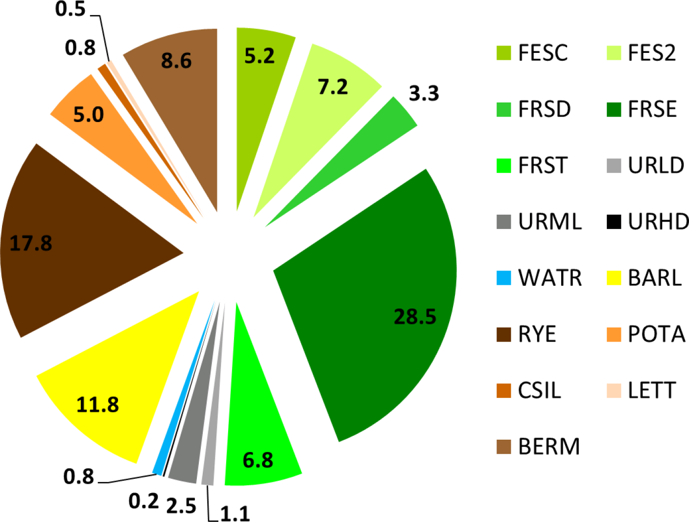
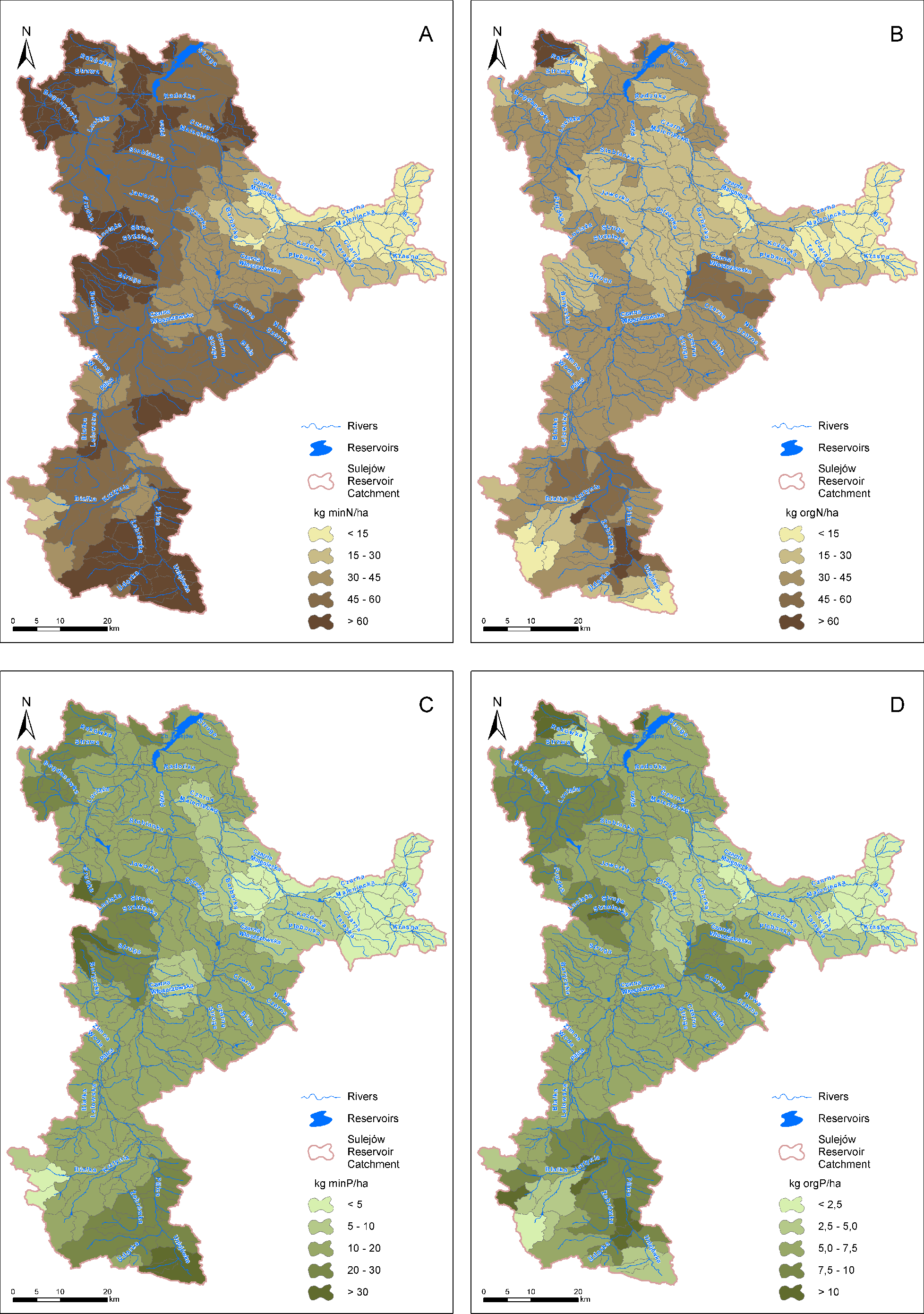


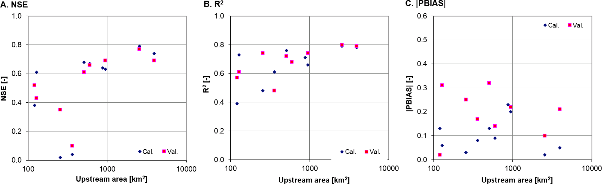


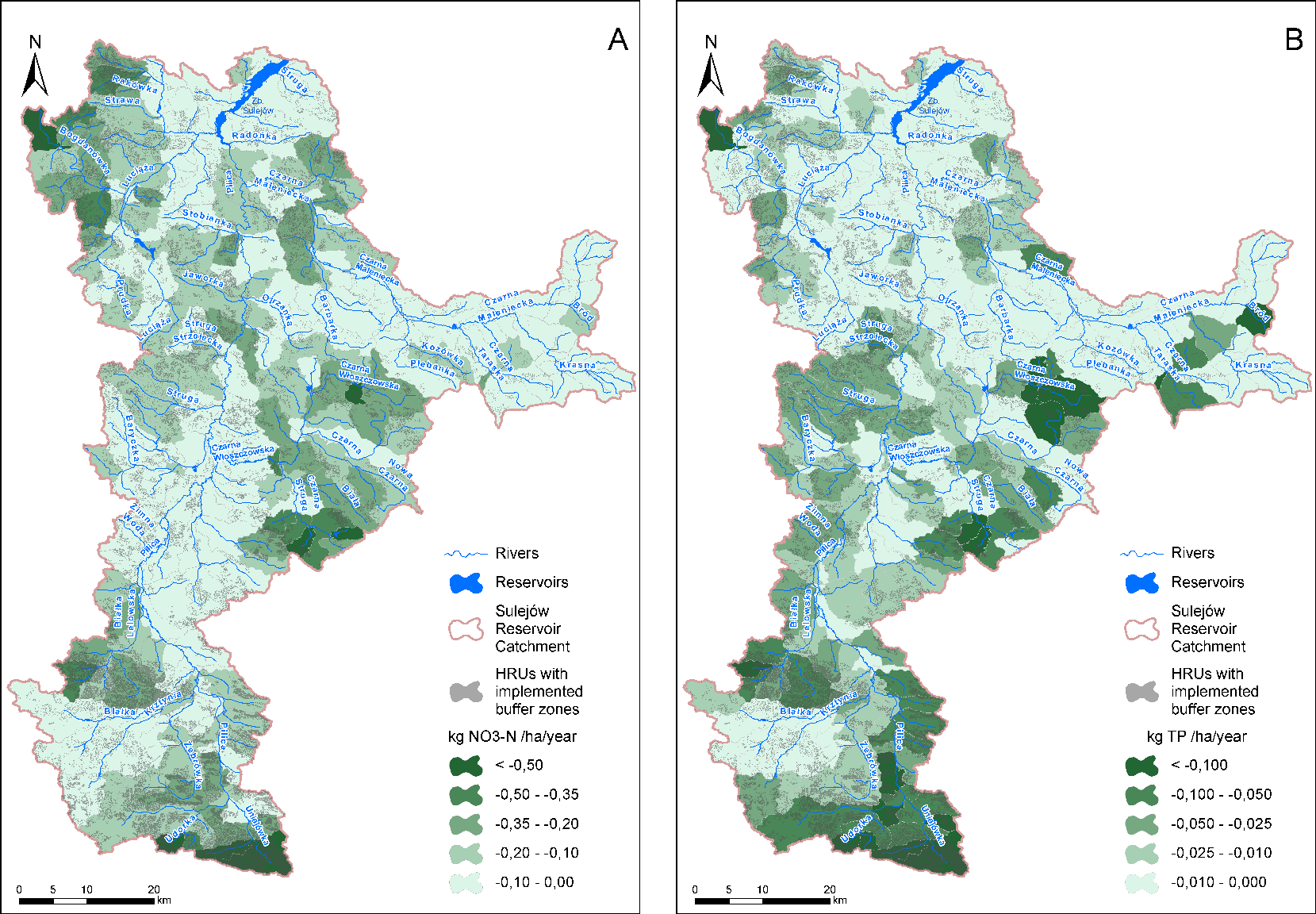

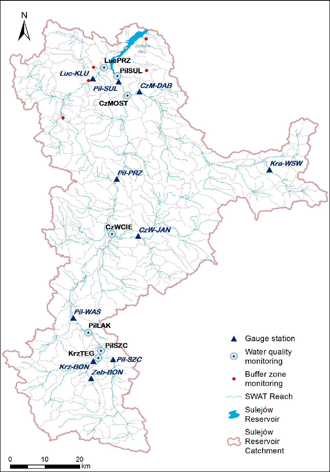
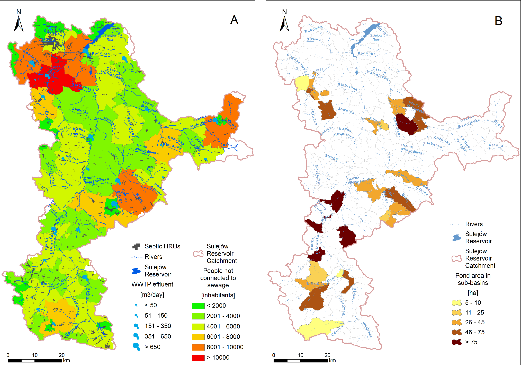
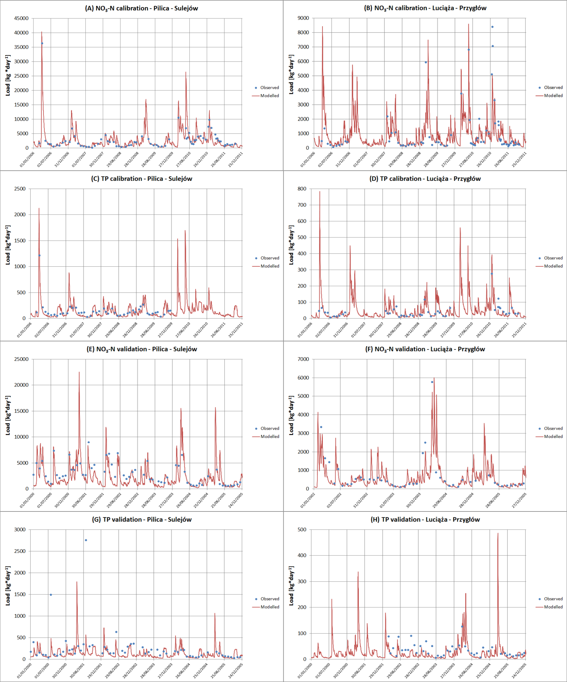
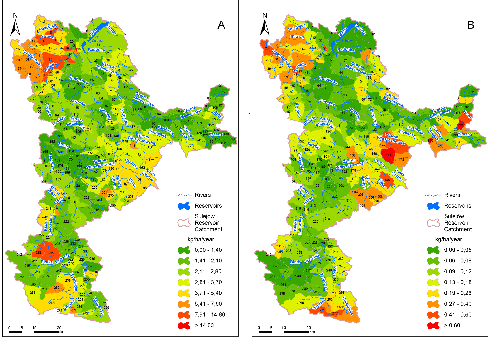
| Data | Source |
|---|---|
| Digital Elevation Model | CODGiK (Central Agency for Geodetic and Cartographic Documentation) |
| Water cadastre GIS layers | RZGW (Regional Water Management Authority in Warsaw) |
| Corine Land Cover 2006 | GDOS (General Directorate of the Environmental Protection) |
| Orthophotomap | GUGiK (Head Office of Geodesy and Cartography: geoportal.gov.pl) |
| Agricultural statistics | The Local Data Bank of GUS (Central Statistical Office) |
| Agricultural soil map 1:100,000 | IUNG-PIB (Institute of Soil Science and Plant Cultivation - National Research Institute) |
| Forest soil maps 1:25,000 | RDLP (Regional Directorate of State Forests in Łódź, Radom and Katowice) |
| Atmospheric deposition of nitrogen | GIOS (Chief Inspectorate of Environmental Protection |
| Climate data | IMGW-PIB (Institute of Meteorology and Water Management - National Research Institute) |
| Pollution Source | TN (kg/year) | TP (kg/year) |
|---|---|---|
| Sewage treatment plants | 81,989 | 6,913 |
| Septic tank effluent | 65,572 | 1,462 |
| Fish pond releases | 53,313 | 9,273 |
| Total | 200,874 | 17,648 |
| Variable | NSE cal. | NSE val. | R2 cal. | R2 val. | PBIAS cal. | PBIAS val. |
|---|---|---|---|---|---|---|
| Discharge | 0.64 | 0.61 | 0.70 | 0.72 | 0.07 | 0.21 |
| NO3–N loads | 0.56 | –0.04 | 0.69 | 0.28 | 0.01 | 0.26 |
| TP loads | 0.48 | 0.08 | 0.71 | 0.25 | 0.05 | 0.47 |
© 2015 by the authors; licensee MDPI, Basel, Switzerland This article is an open access article distributed under the terms and conditions of the Creative Commons Attribution license (http://creativecommons.org/licenses/by/4.0/).
Share and Cite
Piniewski, M.; Marcinkowski, P.; Kardel, I.; Giełczewski, M.; Izydorczyk, K.; Frątczak, W. Spatial Quantification of Non-Point Source Pollution in a Meso-Scale Catchment for an Assessment of Buffer Zones Efficiency. Water 2015, 7, 1889-1920. https://doi.org/10.3390/w7051889
Piniewski M, Marcinkowski P, Kardel I, Giełczewski M, Izydorczyk K, Frątczak W. Spatial Quantification of Non-Point Source Pollution in a Meso-Scale Catchment for an Assessment of Buffer Zones Efficiency. Water. 2015; 7(5):1889-1920. https://doi.org/10.3390/w7051889
Chicago/Turabian StylePiniewski, Mikołaj, Paweł Marcinkowski, Ignacy Kardel, Marek Giełczewski, Katarzyna Izydorczyk, and Wojciech Frątczak. 2015. "Spatial Quantification of Non-Point Source Pollution in a Meso-Scale Catchment for an Assessment of Buffer Zones Efficiency" Water 7, no. 5: 1889-1920. https://doi.org/10.3390/w7051889