Estimation of CN Parameter for Small Agricultural Watersheds Using Asymptotic Functions

Abstract

This paper investigates a possibility of using asymptotic functions to determine the value of curve number (CN) parameter as a function of rainfall in small agricultural watersheds. It also compares the actually calculated CN with its values provided in the Soil Conservation Service (SCS) National Engineering Handbook Section 4: Hydrology (NEH-4) and Technical Release 20 (TR-20). The analysis showed that empirical CN values presented in the National Engineering Handbook tables differed from the actually observed values. Calculations revealed a strong correlation between the observed CN and precipitation (P). In three of the analyzed watersheds, a typical pattern of the observed CN stabilization during abundant precipitation was perceived. It was found that Model 2, based on a kinetics equation, most effectively described the P-CN relationship. In most cases, the observed CN in the investigated watersheds was similar to the empirical CN, corresponding to average moisture conditions set out by NEH-4. Model 2 also provided the greatest stability of CN at 90% sampled event rainfall.

1. Introduction

The runoff amount from an ungauged watershed is one of the basic hydrological parameters used in hydraulic engineering design, flood protection, or in the process of modeling of watershed water balance components [1,2,3,4,5,6,7,8]. Originally, storm water runoff from small agricultural watersheds was estimated using the Soil Conservation Service (SCS) curve number (CN) method, developed by the United State Department of Agriculture (USDA). This method is currently known as the Natural Resources Conservation Service (NRCS)-CN method. Furthermore, its scope has expanded beyond the evaluation of storm runoff and it has become an integral part of more complex, long-term simulation models [9]. This method represents an event-based lumped conceptual approach [10,11,12,13,14,15,16]. In the words of Ponce and Hawkins [17] “The SCS-CN method is a conceptual model of hydrologic abstraction of storm rainfall, supported by empirical data. Its objective is to estimate direct runoff volume from storm rainfall depth, based on a curve number CN”. Despite widespread use of SCS-CN methodology, realistic estimation of the CN parameter has been widely discussed among hydrologists and water resources community [18,19,20,21,22,23,24]. The SCS-CN is a very simple approach developed for predicting surface runoff from hortonian overland flow dominated watersheds. It is straightforward and easy to apply. A primary reason for its wide applicability and acceptability is the fact that it accounts for major runoff generating watershed characteristics, namely soil type, land use/treatment, surface conditions and antecedent moisture conditions (AMC)[4,25,26,27,28,29].

Currently, this method is included in widely used hydrological software, such as WinTR55, WinTR20, HEC-HMS, EPA-SWMM, SWAT, GLEAMS, EPIC, NLEAP, and AGNPS [30], and it is consequently applied in a large number of scientific studies. Isik et al. [31] used a hybrid model based on Artificial Neural Networks (ANNs), and SCS-CN to predict the effect of changes in land use/cover on daily streamflow. Kabiri et al. [32] claimed that runoff values determined by means of the SCS-CN method did not differ from those calculated with the Green-Ampt method. Grimaldi et al. [33,34] proposed a method combining the Green-Ampt infiltration equation and calibration of both the ponding time and soil hydraulic conductivity, using the initial abstraction and total volume given by the SCS-CN method. Sahu et al. [35] verified modified versions of the SCS method to estimate the runoff in agricultural watersheds. The modification involved a different way of determining soil moisture conditions in relation to the original method. Soulis et al. [36] reported a strong correlation between the CN parameter and the precipitation (P) amount, i.e., the more abundant the precipitation, the lower the CN. They also found that flow amount, determined by means of the original method, was markedly overestimated in relation to empirical values and underestimated for scant precipitations. Banasik et al. [37] claimed that application of the SCS-CN method should rely on deep insight into the probabilistic properties of CN and maximum potential retention S. However, estimating watershed runoff based on the original SCS method is disputable. The greatest limitations of the original SCS-CN method include possible sudden jumps in the computed runoff due to using three AMC levels permitting unreasonable sudden jumps in CN, lack of clear guidance on how to vary antecedent moisture conditions, and no explicit dependency between the initial abstraction and the antecedent moisture [35]. Woodward et al. [38] indicated that the SCS-CN method was not applicable at sub-daily time resolution. Hawkins [39] reported that the runoff calculated from the SCS method was much more sensitive to the CN chosen than to rainfall depths. Therefore, error analysis and sensitivity calculus seem to indicate that errors in CN affect the runoff calculation to a much greater extent than errors in the storm rainfall. Next, it is difficult to correctly select CN_s from available handbook tables. CN_s from the handbook tables is most successfully estimated for traditional agricultural watersheds, less successfully for semiarid rangelands and the least successfully for forest watersheds. Numerous studies on the application of the original SCS-CN method for calculating effective rainfall [40,41,42] showed that CN parameter values, specified theoretically and according to SCS guidelines, differed significantly from those calculated empirically, based on recorded rainfall-runoff events. Apart from variable watershed moisture conditions, the CN parameter is also affected by precipitation abundance, which is not accounted for in the original method. In his study on asymptotic determination of runoff curve numbers from measured runoff, Hawkins [39] concluded that a secondary systematic correlation usually emerged in watersheds between the calculated CN value and the rainfall depth. In most watersheds, the calculated CN_s approaches a constant value with increasing rainfall depth that is assumed to characterize a specific watershed. The three different patterns of the CN-P relationship can be described as follows: the most common scenario is that small rainfall depths correspond to greater values of calculated CN_s, which decline progressively with increasing storm size, approaching a stable near constant asymptotic CN value with increasingly larger storms. This behavior occurs most frequently and it is deemed “standard”. In less common cases, the observed CN declines steadily with increasing rainfall, with no appreciable tendency to approach a constant value (“complacent” behavior). In the last case, also concerning a small number of watersheds, the calculated CN_s has an apparently constant value for all rainfall depths, except for very low rainfall depths where CN increases suddenly (“violent” behavior). Soulis et al. [43,44], used a two-CN heterogeneous system for calculating watershed runoff. They found that in the watersheds characterized by heterogeneous land use, the runoff determined with this approach was very similar to the actually recorded runoff. They also demonstrated that the runoff calculated with the proposed method allowed—irrespective of the adopted λ value—a more accurate runoff evaluation as compared with the original SCS-CN method. Unfortunately, many designers unknowingly use the original method in their hydrological calculations, which can result in a significant underestimation of the actual flood parameters. Therefore, it seems necessary to verify the application of the SCS-CN approach in local conditions, to reduce the uncertainty of modeling results and to promote more common use of this method in practice.

The aim of the study was to assess the applicability of asymptotic functions for determining the value of the CN parameter as a function of precipitation depth in small agricultural watersheds. Additionally, a comparative analysis of the computed CN values and those provided by SCS National Engineering Handbook Section 4(NEH-4) Hydrology and Technical Release 20 (TR-20) was carried out. The methodological basis of this work was the research published by Hawkins [39]. The methods described there were supplemented with so far uncommonly used asymptotic functions such as kineticsfunction and complementary error function peak from the set of symmetric functions.

2. Materials and Methods

The study was conducted in four small watersheds, two of which (A and D) are located in Gaj, the municipality of Mogilany, Krakow district, and the two other (B and G) in the municipality of Andrychów, Wadowice district. All the watersheds are located in southern Poland, with A and D belonging to the eastern section of the Wieliczka Foothills, and B and G to the eastern part of the Little Beskids [7]. In hydrographic terms, the A and D watersheds belong to the drainage area of the river Wilga, the right tributary of the Vistula, and B and G to the drainage area of the Wieprzówka, the right tributary of the Skawa.

The watersheds are characterized by regular shapes, and differ in their area, average length, above sea level, unit length of the watercourse per 1 km², average land slope, and length of watercourses. The watersheds of D and G are of the same width. The mean slope of the watershed B is 9.9%, with dominant values within a 5 to 10% range, while in the watershed G (mean slope 12.2%), the dominant slope range is 10% to 18%. In both watersheds, the slopes account for about 40% of their areas. Slopes exceeding 27% account for 4% and 9% of B and G watershed area, respectively. The watersheds of A and D also differ in terms of slope distribution. The high share of the slope exceeding 27% in the watershed D is worth noting, accounting for 6% of its area. The watershed A is dominated by the slopes ranging from 5% to 18% and covering nearly 68% of its area. In the watershed D, the slopes within the range of 10% to 27% cover over 56% of its area (Table 1 and Figure 1).

The watersheds of A and D are covered with luvisols, eutriccambisols and eutricstagniccambisols, developed from loesses and loess-like substrates. In terms of soil type, they are silts and clayey silts. They are usually characterized by unfavorable air-water relations. Except for the topsoil, they are poorly compacted soils.

Table 1. Basic physiographic and use-related characteristics of the investigated watersheds.

Parameter	Watershed
	A	D	B	G
Watershed area F [km2]	0.364	0.546	0.274	0.475
Length Lz [km]	0.525	1.200	1.150	1.000
Width S [km]	0.750	0.525	0.290	0.525
Altitude H [m a.s.l.]	277–325	271–327	396–481	396–457
Mean altitude [m]	299	300	424	425
Mean slope Iśr [%]	10.7	12.3	9.9	12.2
Length of watercourse [km]	0.386	1.000	1.210	0.575
Density of hydrographic network ρ [km·km−2]	1.72	1.83	4.40	1.21
Mean precipitation in multi-year (1951–2000) period P [mm]	663		898
Land use [%]	A	D	B	G
Arable land	51.4	56.2	64.6	70.7
Grassland	25.6	11.4	27.4	16.9
Forests	1.9	9.3	--	8.4
Orchards	8.2	5.5	1.5	--
Urban area and wastelands	12.9	17.6	6.5	4.0

Table 1. Basic physiographic and use-related characteristics of the investigated watersheds.

Parameter	Watershed
	A	D	B	G
Watershed area F [km2]	0.364	0.546	0.274	0.475
Length Lz [km]	0.525	1.200	1.150	1.000
Width S [km]	0.750	0.525	0.290	0.525
Altitude H [m a.s.l.]	277–325	271–327	396–481	396–457
Mean altitude [m]	299	300	424	425
Mean slope Iśr [%]	10.7	12.3	9.9	12.2
Length of watercourse [km]	0.386	1.000	1.210	0.575
Density of hydrographic network ρ [km·km−2]	1.72	1.83	4.40	1.21
Mean precipitation in multi-year (1951–2000) period P [mm]	663		898
Land use [%]	A	D	B	G
Arable land	51.4	56.2	64.6	70.7
Grassland	25.6	11.4	27.4	16.9
Forests	1.9	9.3	--	8.4
Orchards	8.2	5.5	1.5	--
Urban area and wastelands	12.9	17.6	6.5	4.0

Permeability (ω) of these soils, one of the crucial hydrologic parameters, is 0.2 < ω <1.0 m∙day⁻¹ in the topsoil (0–28 cm) and less than 0.05 m∙day⁻¹ in the subsoil layer. The watersheds of B and G are covered with relatively shallow, skeletal brown soils of acid and eutric type, formed from flysch rock mass. The content of skeleton particles is between 20% and 50%. These are mainly silty clays, clayey silts (G), and light and heavy loams (B), containing from 32% to 58% of fine particles and from 28% to 45% of silt particles. Permeability of the topsoil (0–21cm) is 0.2 < ω < 2.0 m∙day⁻¹, and for the subsoil (21–72 cm) it is 0.05 < ω < 0.2 m∙day⁻¹.

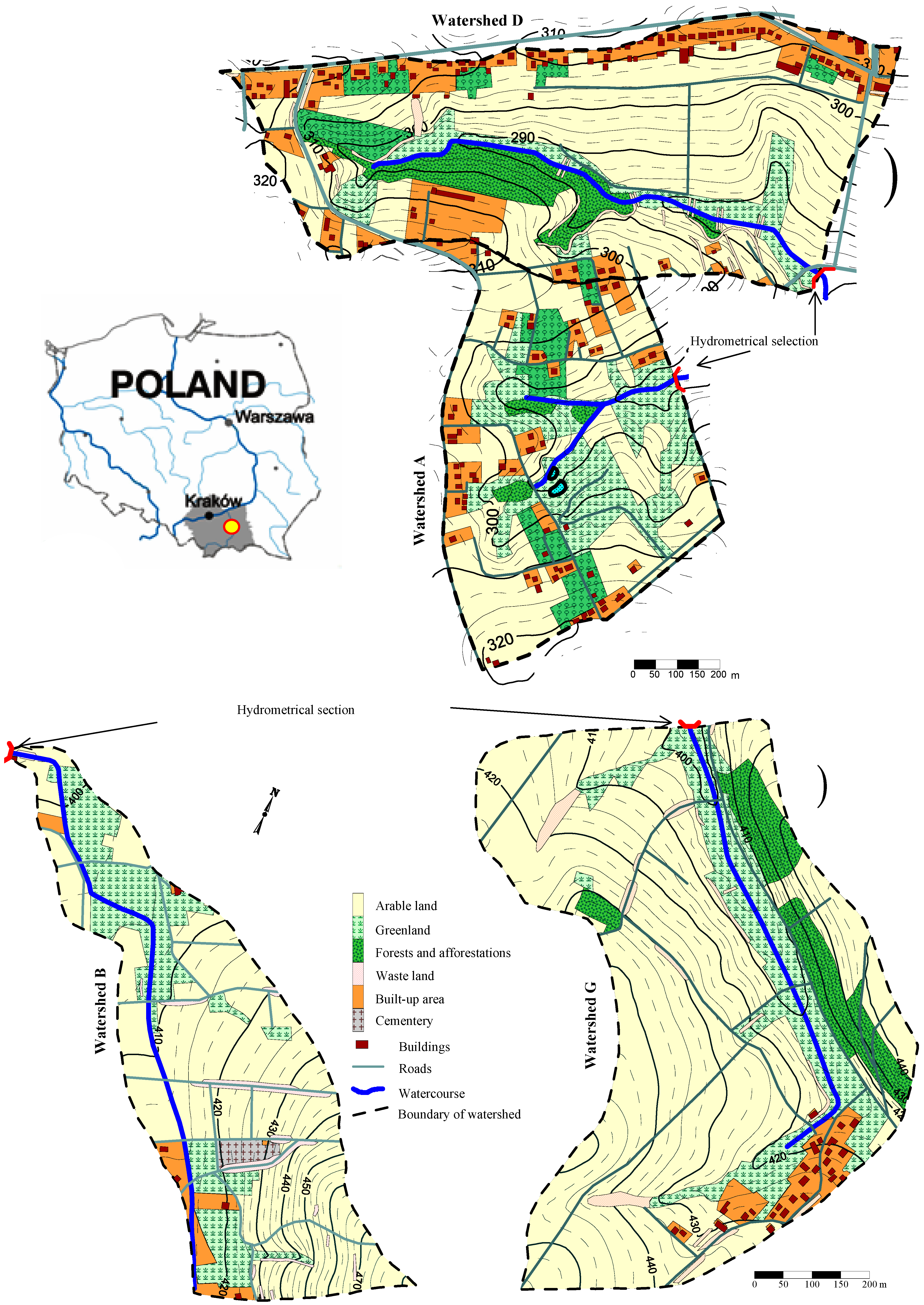
Figure 1. Investigated watersheds.

Figure 1. Investigated watersheds.

The watershed lands are mostly used for agriculture, with predominance of arable lands. Their share is from 51.4% in the watershed A to nearly 71% in G. Grasslands account for 11.4% of the watershed D, and up to 27.4% of the watershed B (Table 1 and Figure 1).

The study was performed in the hydrologic years 2001–2006 for the watersheds A, D and B, and between 2001 and 2011 for the watershed G. Twenty rainfall-runoff episodes were analyzed for A, D and B watersheds and 54 in the watershed G. Rainfall and runoff were monitored on a regular basis. Rainfall was measured using a pluviometer with an option of continuous recording, located within the investigated watersheds.

The research included two rainfall stations, the first of which was located near the watersheds of A and D, and the second covered the other two watersheds (B and G). While computing, the same rainfall values were used for the watersheds covered by the same rainfall stations. Runoff was determined based on a limnigraph on triangular and trapezoidal weirs. Knowing the parameters of the weir rating curves, tared at the hydraulics laboratory at the University of Agriculture in Krakow, it was possible to calculate the runoff (mm) for specific rainfall events. The rainfall and runoff events were measured following 30-minute intervals.

Further analysis accounted for direct runoff, determined as the difference between the total (measured) runoff and the baseflow. The baseflow was separated from discharge using the straight-line method.

2.1. Characteristics of the SCS-CN Method

The SCS-CN method is based on the water balance equation and two fundamental hypotheses. The first hypothesis equates the ratio of actual amount of direct surface runoff Q to the total rainfall P (or maximum potential surface runoff) to the ratio of actual infiltration (F) to the amount of the potential maximum retention S. The second hypothesis relates the initial abstraction (Ia) to the potential maximum retention S [4]. A popular form of the SCS-CN method is expressed as:

$$Q=\frac{{(P-I_a)}^2}{P-I_a+S}ifP>I_a$$

(1)

Q = 0 otherwise

$$I_a=\lambda S$$

(2)

where Q—Direct runoff (mm), P—Total precipitation (mm), I_a—initial abstraction (mm), S—Potential maximum retention (mm) and λ—Initial abstraction coefficient (dimensionless).

2.2. Calculation Procedure

Preliminary calculations for each watershed included determining the values of empirical CN (CN_emp), based on the tables provided in the NEH-4 [14]. Runoff was calculated using Equation (1), taking into account three levels of soil moisture, watershed land use and soil conditions. Following NEH-4 guidelines, it was assumed that λ = 0.20. Next, observed CN (CN_obs) was determined for each investigated watershed, using the recorded rainfall-runoff (P-Q) episodes. To this end, S_i retention volume for each P-Q pair was calculated using the equation [39]:

$$S_i=5\left[P_i+2Q_i-\sqrt{4Q_i^2+5P_i{Q}_i}\right]$$

(4)

and then CN_obs was computed:

$$C{N}_{obs}=\frac{25400}{254+S_i}$$

(5)

where P_i—Total precipitation of an event [mm], Q_i—Direct runoff [mm].

Then, the measured P and Q values for each watershed were sorted separately and realigned on a rank order basis to form P-Q pairs of equal return period, following the frequency matching technique [39]. After that, the measured P-Q data were transformed into the equivalent P-CN_obs data using Equation (5). Three models were used to describe CN_obs parameter as a function of rainfall amount (P):

• Standard asymptote model described by Hawkins [39]:

  $$CN(P)1=C{N}_{\infty }+\left(100-C{N}_{\infty }\right)\cdot \exp (-k\cdot P)$$

  (6)

  where CN_∞—A constant approached as P→∞, k—fitting constant.
• Kinetics equation using the decay function:

  $$CN(P)2=C{N}_L+{\left[b^{1-d}+c\cdot P(d-1)\right]}^{\frac{1}{1-d}}$$

  (7)

  where CN_L is a curve number for large P, b is decay function, c and d—Are fitted constants.
• Complementary error function peak from the set of symmetric functions:

  $$CN(P)3=C{N}_{\infty }+b\cdot erfc\left[{\left(\frac{P-c}{d}\right)}^2\right]$$

  (8)

  where CN_∞ is a constant approached as P→∞; b is amplitude of density function, c—Location parameter, d—Scaling parameter. Equations (6)–(8) and the parameter values were determined using Table Curve 2D software [45].

In the present study, we used the root mean square error (RMSE), Nash-Sutcliffe model efficiency (EF) [46], and determination coefficient r² as model goodness of fit to assess the model performance. RMSE and EF were expressed as below:

$$RMSE=\sqrt{\frac{1}{N}{\displaystyle \sum _{i=1}^N{(Q_{obs,i}-Q_{calc,i})}^2}}$$

(9)

$$EF=1-\frac{{\displaystyle {\sum }_{i=1}^N{(Q_{obs,i}-Q_{calc,i})}^2}}{{\displaystyle {\sum }_{i=1}^N{(Q_{obs,i}-\overline{Q_{obs}})}^2}}$$

(10)

where RMSE is in mm, EF is dimensionless. Q_obs is the observed storm runoff (mm), Q_calc is the calculated runoff (mm), $\overline{Q_{obs}}$ is a mean of the observed runoff values in the catchment, N is the total number of rainfall-runoff events, and i is an integer varying from 1 to N.

3. Results and Discussion

Main characteristics of the analyzed catchments, determined by means of regular monitoring of rainfall and runoff events, are presented in Table 2. The greatest mean precipitation during an episode, amounting to 85.4 mm, was observed in the watershed B, and it accounted for 9.5% of an average annual precipitation for a multi-year period (85.4 mm/898 mm = 9.5%). The lowest precipitation was recorded in the watershed G (51.6 mm), where it accounted for only 5.7% of an average annual precipitation (51.6 mm/898 mm = 5.7%). As A and D watersheds, both belonging to the drainage area of the Wilga, are very close to each other, and the precipitation data from the same rainfall stations were used, the amount of precipitation in these watersheds was identical. A similar situation occurred for B and G watersheds that are subwatersheds of the Skawa. The greatest precipitation variability during runoff triggering episodes (P_max-P_min) was found in the watershed G and it was 299.6 mm, while the smallest variability was noticed in the watersheds A and D—258.0 mm. Precipitation amount clearly correlated with runoff height, and therefore the largest runoff during a flood occurred in the catchment B—an average of 38.4 mm, and the smallest in the catchment G—15.1 mm. The CN parameter is a crucial one when determining the runoff amount in the SCS-CN method [47,48]. CN_obs was calculated using Equation (5), based on the recorded rainfall-runoff episodes. The highest mean value of CN_obs, amounting to 78.1, was observed in the watershed G, and the lowest in the watershed D (71.8). The watershed Gis dominated by arable lands (70.7% of its area), and its storage capacity was limited, which could cause an increase in the CN_obs parameter. However, this observation requires verification by means of an analysis of changes to CN parameter against precipitation, as discussed below. Equally high values of CN_obs were found for the watershed B. This watershed is also characterized by limited storage capacity, as most of its area (64.4%) is covered by arable lands. A substantial share of built-up land (6.5% of total watershed area) also played an important role.

Table 2. Characteristics of the rainfall-runoff events for all watersheds.

Watershed	P Average [mm]	Range Pmin–Pmax [mm]	Q Average [mm]	Range Qmin–Qmax [mm]	CNobs_average	Range CNobs_min–CNobs_max
A	65.8	17.0–275.0	21.7	1.3–191.6	75.5	59.5–90.6
B	85.4	21.1–297.5	38.4	4.0–217.2	77.4	53.8–96.7
D	65.8	17.0–275.0	19	1.3–222.4	71.8	51.5–97.6
G	51.6	6.6–306.2	15.1	0.02–178.7	78.1	55.2–96.6

Table 2. Characteristics of the rainfall-runoff events for all watersheds.

Watershed	P Average [mm]	Range Pmin–Pmax [mm]	Q Average [mm]	Range Qmin–Qmax [mm]	CNobs_average	Range CNobs_min–CNobs_max
A	65.8	17.0–275.0	21.7	1.3–191.6	75.5	59.5–90.6
B	85.4	21.1–297.5	38.4	4.0–217.2	77.4	53.8–96.7
D	65.8	17.0–275.0	19	1.3–222.4	71.8	51.5–97.6
G	51.6	6.6–306.2	15.1	0.02–178.7	78.1	55.2–96.6

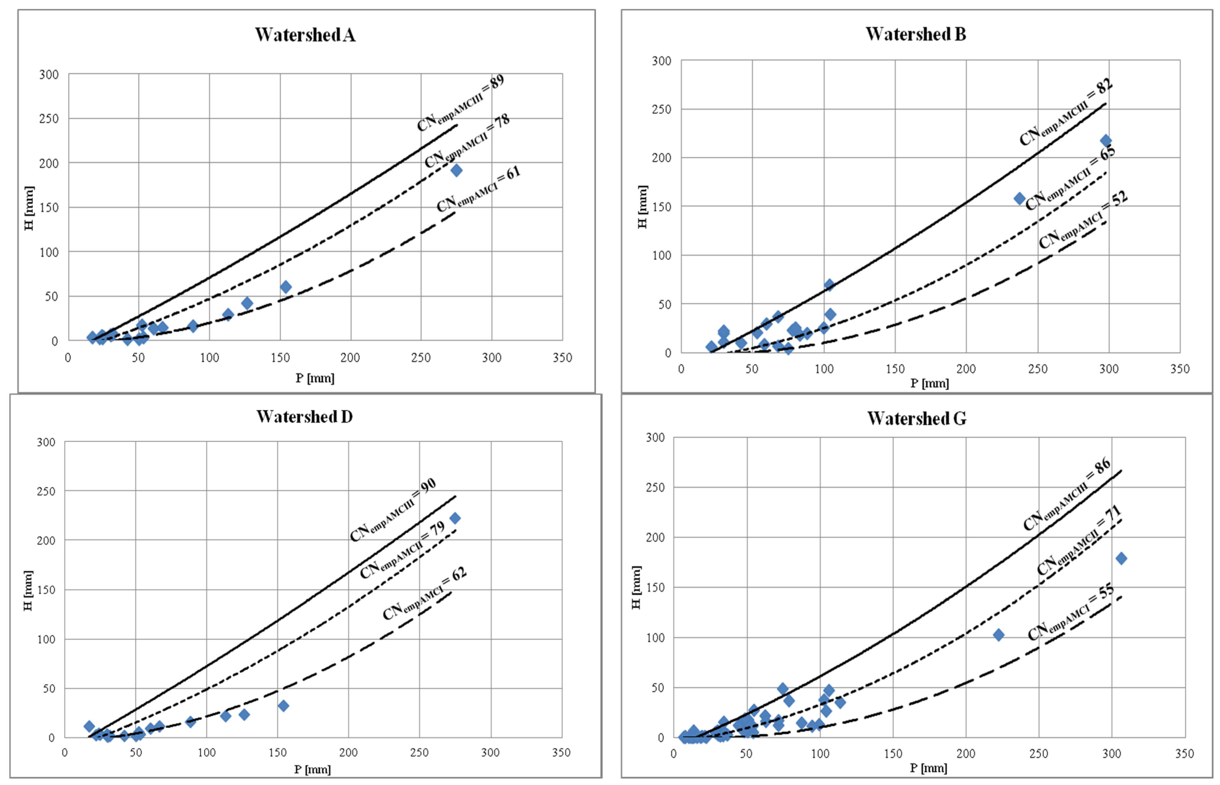
The recorded rainfall-runoff episodes were compared with the runoff calculated according to the original SCS-CN method—Equations (1) to (3). CN_emp was determined based on watershed land use and soil conditions for three levels of soil moisture. Runoff values for CN_emp corresponding to AMC I and II were calculated as follows: first, CN_emp for individual categories of land use and soil type were determined for normal conditions (AMCII). Then, average weighted value of CN_empAMCII for a specific watershed for AMCII was calculated. NEH-4 tables and previously determined values of CN_emp for specific land use and soil categories were used to work out CN_emp for dry (AMCI) and moist (AMCIII) conditions and then average weighted values of CN_empAMCI and CN_empAMCIII for the watershed were calculated. The determined weighted means of CN_emp for different moisture levels and Equations (1) and (3) were used to calculate runoff for variable precipitation P.

The outcomes are presented in Figure 2. They indicate that for each of the analyzed watersheds, the measured rainfall and runoff amounts fall within the theoretical curves limited by extreme levels of moisture. In the watersheds A and D the recorded values were usually located near the curve for the first, i.e., the lowest antecedent moisture level (AMCI). This tendency for concentrating runoff measurements near the curve for the lowest moisture soil conditions was identified mainly for less abundant precipitations. During higher rainfalls, the runoff was located near the curve representing normal (AMCII) condition. In the watersheds B and G, for precipitation P < 150 mm, the values of the measured runoff were located between the upper curve representing AMCIII and the bottom curve representing AMCI, and were not concentrated around any specific curve. For higher precipitation amounts, the runoff values approached the curve representing normal moisture conditions AMCII. Another pattern resulted from a comparison of CN_obs and CN_emp. A comparison of average values of CN_obs presented in Table 2 with CN_emp for various moisture levels (Figure 2) demonstrated that in the watersheds of D and G, CN_emp for AMCII was markedly higher than the average CN_obs determined based on the recorded rainfall-runoff episodes, and in the watershed B CN_emp for AMCII was lower than the average CN_obs. It can be therefore concluded that determining a direct runoff according to the original SCS-CN method and assuming CN provided in the NEH-4 tables, may result in significant underestimation or overestimation of the runoff for normal moisture conditions, and consequently underestimation or overestimation of the design flow rates. This means that, in the case of the investigated watersheds, the rainfall reached already moist soil. The watershed soil moisture level was affected not only by precipitation, but also by a high level of ground water table that could be maintained after the winter period, leading to a reduced watershed retention capacity, as well as a poorly permeable substrate that made precipitation infiltration more difficult. Similar observations concerning the differences between CN_emp are presented in the NEH-4 tables, and its observed values have been reported in other papers [40,42,49,50]. These differences between CN_emp and CN_obs may be explained by the fact that CN_emp values provided in the NEH-4 were specified for fairly flat agricultural watersheds (with a slope of up to 5%) [4], characterized by a much higher retention capacity than those investigated in this study. Moreover, in the original method, CN was determined based on maximum daily precipitation per year, and in our study this parameter was calculated using the rainfall causing direct runoff from the investigated watersheds. De Paola et al. [30] suggest using the AMCIII class for flow predictions when designing “sensible’ structural hydraulic measures (such as detention reservoirs or floodplain storage), while for non-structural measures (such as delineation of hazard maps) this assumption may be too severe and, therefore, it requires a precise evaluation of its occurrence frequency. To adapt the SCS method for use in mountain or highland watersheds, it has been proposed [4] to correct CN_emp by a factor representing the watershed slope.

Figure 2. The relationship between runoff Q and rainfall P depth and calculated runoff values for the empirical CN (CN_emp) for three antecedent moisture conditions in the investigated watersheds.

Figure 2. The relationship between runoff Q and rainfall P depth and calculated runoff values for the empirical CN (CN_emp) for three antecedent moisture conditions in the investigated watersheds.

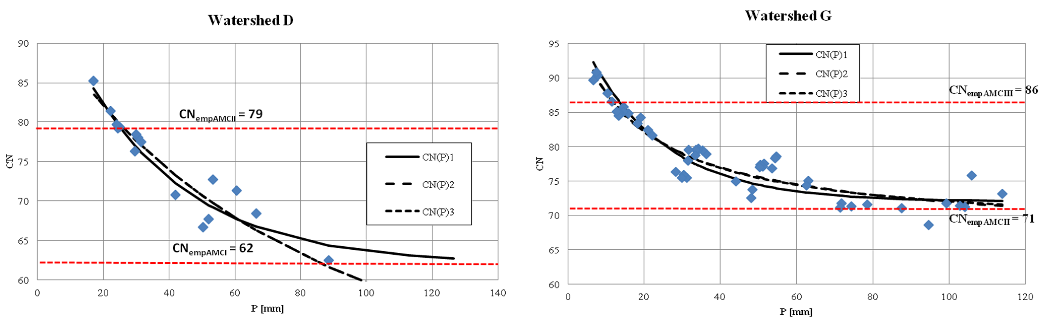
Another problem was to determine the effect of precipitation depth on CN_obs. Figure 3 presents the rainfall-runoff pairs after an application of a frequency matching technique. In addition, the recorded data were approximated with the proposed models, described by the Equations (6) to (8). Distribution of the dots in Figure 3 indicates a strong secondary relationship between the curve number and rainfall depth, i.e., CN_s values decrease with the increase of rainfall depth. The watersheds of A, B and G showed a tendency to CN_obs parameter stabilization for extremely high precipitations. This tendency has been observed in a majority of watersheds [39].

Figure 3. The relationship of the observed CN (CN_obs) and precipitation P (dots), with approximation of asymptotic functions CN(P) by Equations (6) to (8); dashed horizontal lines represent CN_emp values for selected moisture levels (antecedent moisture conditions, AMC) according to National Engineering Handbook Section 4 NEH-4).

Figure 3. The relationship of the observed CN (CN_obs) and precipitation P (dots), with approximation of asymptotic functions CN(P) by Equations (6) to (8); dashed horizontal lines represent CN_emp values for selected moisture levels (antecedent moisture conditions, AMC) according to National Engineering Handbook Section 4 NEH-4).

The authors of this study hypothesized that the course of the P-CN_obs relationship may be due to different runoff triggering processes, such as overland flow and rapid subsurface flow. For a small rainfall to cause a surface runoff, the precipitation duration usually needs to be short, and a watershed must be characterized by a high moisture level or poor permeability. As a result, small precipitations are associated with high CN_obs values. However, high values of CN_obs during small precipitation may also occur when the rain reaches the soil covered with a non-permeable layer formed due to long-lasting drought. If this happens, the rain, at least in its initial phase, will not infiltrate the soil profile but will form a surface runoff. As a result, high CN_obs values may be recorded for even small precipitations. In the case of extremely high and prolonged rainfalls, the runoff may be caused by various reasons (overland flow, subsurface flow etc.), and the substrate permeability is less important than during small precipitations. An important factor is also the flow time in a river network. In the case of longer rainfalls, total runoff is additionally affected by underground river supply. Spatial variations in watershed characteristics, mainly land use, can also shape the CN_obs-P relationship [43,44]. The investigated watersheds are characterized by variable land use, with a dominant share of arable lands and urban areas featuring low potential retention capacity and smaller areas of higher retention capacity and higher ability to delay the runoff, i.e., grasslands and forests. These factors make CN_obs parameter values decline and steady during high rainfalls. Hawkins [39] proposed the use the asymptotic functions for approximation of CN_obs vs. P relationship, after applying a sorting technique to the measured data. The authors of this paper followed the methodological assumptions presented by Hawkins. The parameters of the proposed functions and quality assessment of model fit to the observational data for each investigated watershed are presented in Table 3, Table 4, Table 5 and Table 6.

Table 3. P-CN_obs parameters of different models and the quality of calculation-observation fit in the watershed A.

Model	Parameters	E [%]	RMSE (-)	R 2, *	A (90) ** [%]
CN(P)1	CN∞ = 62.00; k = 42.18	88.10	2.42	0.89	50.00
CN(P)2	CNL = 64.20; b = 24.81; c = 0.28; d = 0.00	95.70	2.05	0.92	99.90
CN(P)3	CN∞ = 63.90; b = 26.21; c = −3236.00; d = 109.16	90.80	2.14	0.91	80.00

Notes: * Determination coefficient; ** percent attainment of CN_∞ or CN_L at 90% sampled event rainfall.

Table 3. P-CN_obs parameters of different models and the quality of calculation-observation fit in the watershed A.

Model	Parameters	E [%]	RMSE (-)	R 2, *	A (90) ** [%]
CN(P)1	CN∞ = 62.00; k = 42.18	88.10	2.42	0.89	50.00
CN(P)2	CNL = 64.20; b = 24.81; c = 0.28; d = 0.00	95.70	2.05	0.92	99.90
CN(P)3	CN∞ = 63.90; b = 26.21; c = −3236.00; d = 109.16	90.80	2.14	0.91	80.00

Notes: * Determination coefficient; ** percent attainment of CN_∞ or CN_L at 90% sampled event rainfall.

Table 4. P-CN_obs parameters of different models and the quality of calculation-observation fit in the watershed B.

Model	Parameters	E [%]	RMSE (-)	R 2,*	A (90) ** [%]
CN(P)1	CN∞ = 71.50; k = 38.01	89.60	1.56	0.93	30.00
CN(P)2	CNL = 72.10; b = 23.57; c = 0.11;d = 0.407	96.50	1.27	0.93	99.90
CN(P)3	CN∞ = 70.40; b = 57.97;c = −737.00 d = −55.22	93.00	1.28	0.93	20.00

Notes: * Determination coefficient; ** percent attainment of CN_∞ or CN_L at 90% sampled event rainfall.

Table 4. P-CN_obs parameters of different models and the quality of calculation-observation fit in the watershed B.

Model	Parameters	E [%]	RMSE (-)	R 2,*	A (90) ** [%]
CN(P)1	CN∞ = 71.50; k = 38.01	89.60	1.56	0.93	30.00
CN(P)2	CNL = 72.10; b = 23.57; c = 0.11;d = 0.407	96.50	1.27	0.93	99.90
CN(P)3	CN∞ = 70.40; b = 57.97;c = −737.00 d = −55.22	93.00	1.28	0.93	20.00

Notes: * Determination coefficient; ** percent attainment of CN_∞ or CN_L at 90% sampled event rainfall.

Table 5. P-CN_obs parameters of different models and the quality of calculation-observation fit in the watershed D.

Model	Parameters	E [%]	RMSE (-)	R 2, *	A (90) ** [%]
CN(P)1	CN∞ = 62.00; k = 32.00	87.10	2.81	0.90	--
CN(P)2	CNL = 21.90; b = 72.05; c = 0.00; d = 2.29	97.30	1.78	0.95	--
CN(P)3	CN∞ = 49.10; b = 303.45; c = −14,832.00; d = −135.85	94.40	1.84	0.94	--

Notes: * Determination coefficient; ** percent attainment of CN_∞ or CN_L at 90% sampled event rainfall.

Table 5. P-CN_obs parameters of different models and the quality of calculation-observation fit in the watershed D.

Model	Parameters	E [%]	RMSE (-)	R 2, *	A (90) ** [%]
CN(P)1	CN∞ = 62.00; k = 32.00	87.10	2.81	0.90	--
CN(P)2	CNL = 21.90; b = 72.05; c = 0.00; d = 2.29	97.30	1.78	0.95	--
CN(P)3	CN∞ = 49.10; b = 303.45; c = −14,832.00; d = −135.85	94.40	1.84	0.94	--

Notes: * Determination coefficient; ** percent attainment of CN_∞ or CN_L at 90% sampled event rainfall.

Table 6. P-CN_obs parameters of different models and the quality of calculation-observation fit in the watershed G.

Model	Parameters	E [%]	RMSE (-)	R 2, *	A (90) ** [%]
CN(P)1	CN∞ = 72.00; k = 20.55	87.50	2.02	0.89	99.00
CN(P)2	CNL = 64.30; b = 38.70; c = 0.00; d = 2.58	90.00	1.80	0.90	20.00
CN(P)3	CN∞ = 67.70; b = 124.75; c = −1220.00; d = −12.35	90.00	1.80	0.90	30.00

Notes: * Determination coefficient; ** percent attainment of CN_∞ or CN_L at 90% sampled event rainfall.

Table 6. P-CN_obs parameters of different models and the quality of calculation-observation fit in the watershed G.

Model	Parameters	E [%]	RMSE (-)	R 2, *	A (90) ** [%]
CN(P)1	CN∞ = 72.00; k = 20.55	87.50	2.02	0.89	99.00
CN(P)2	CNL = 64.30; b = 38.70; c = 0.00; d = 2.58	90.00	1.80	0.90	20.00
CN(P)3	CN∞ = 67.70; b = 124.75; c = −1220.00; d = −12.35	90.00	1.80	0.90	30.00

Notes: * Determination coefficient; ** percent attainment of CN_∞ or CN_L at 90% sampled event rainfall.

The results in the tables indicate that the best outcomes in all the analyzed watersheds were obtained from the kinetic model described by Equation (7). Its effectiveness ratio E ranged from 90.0% to 97.3%. Assuming the criteria presented by Moriasi et al. [51], this model should be deemed very good. Comparable results were achieved by Banasik et al. [52], who investigated similar functions in an urbanized watershed in Warsaw (central Poland). The standard model developed by Hawkins, commonly used to describe P-CN_obs relationships, provides in fact the least accurate description. The same is true for RMSE, the lowest value of 1.27 was observed in the watershed B for Model 2, and the highest (2.81) in the watershed D for the standard model described by the Equation (7). Very high coefficients of determination (r²) were achieved for all the analyzed watersheds and functions. Despite very good quality of the approximating functions for the P-CN_obs data in the watershed D, the amount of runoff should still be estimated using a simplified linear model and not Equation (1). This is due to the fact that variable values of CN_obs during high rainfalls make it impossible to determine CN_∞ or CN_L [39]. Lack of stability of CN_obs parameter in the watershed D might be due the watershed aspect. As much as 67% of its area face south, which is conducive to significant evaporation from the soil surface (Figure 1). However, this assumption requires further verification. Another reason might be the high density of the hydrographic network in the watershed D (Table 1). This may lead to a much shorter concentration time due to a dominant share of channel flow, finally resulting in increased underground supply of a watercourse and changed shape of the runoff hydrograph. Therefore, it can be concluded that the watershed D is an example of variability of the CN_obs-P pairs, defined by Hawkins [39] as “complacent behavior”. Hawkins claimed the complacent behavior might be observed in 16% of investigated agricultural watersheds. Such a pattern of CN_obs-P relationship also seems possible in watersheds with considerable share of urban areas, like the watershed D, where they account for nearly 18% of its surface. In the other watersheds, the CN_obs-P relationship followed the “standard behavior” pattern, which is the most common. According to Hawkins, it is observed in 70% of all watersheds and has also been reported in this study in mountain and sub-mountain watersheds located in moderate climate zone.

The parameters of CN_∞ or CN_L play a key role in the proposed functions, and they may provide alternative values for CN_emp determined from NEH-4 tables. In the watershed A, CN_∞ and CN_L ranged from 62 to 64.2 and corresponded to CN_emp = 61 for AMCI. For AMCII, the moisture level most often adopted by designers, CN_∞ and CN_L are lower than 20% and 18%. Therefore, adopting CN_∞ or CN_L as design values may cause underestimation of the runoff amount for maximum rainfall as compared to the original method. In the watershed B, CN_∞ and CN_L ranged from 70.4 to 72.1 and exceeded CN_emp for AMCII by about 10%. In the watershed G, CN_∞ and CN_L ranged from 64.3 to 72 and were similar to CN_emp for AMCII. Considering the previously mentioned limitations that resulted in achieving unrealistic CN_∞ and CN_L in the watershed D (Figure 3), no such comparison was made in this case. Comparison of the proposed functions revealed that CN values for extreme rainfalls were similar, and except for the watershed G (the watershed D was excluded due to lack of CN_obs stabilization during high precipitation), the highest values were obtained for the kinetic model. Therefore, it can be generally concluded that in the case of the investigated watersheds, CN_∞ and CN_L parameters were similar to CN_emp, corresponding to average moisture conditions set out by NEH-4. Using CN_∞ or CN_L as a referential CN in design works is based on an assumption that the constant CN = CN_∞ or CN_L is approached closely for the larger extreme events. Since most data sets cover periods of records much shorter than design-return periods, safe extrapolation of the fitted P-CN_obs relations must be a concern. This is a general problem with extending model results beyond measured data, and it is not limited to this method. However, two measures of confidence were proposed by Hawkins [39]: A(90)—percent attainment of CN_∞ or CN_L at 90% sampled rainfall event and S(90)—computed slope in percent of P-Q relationship at 90% sampled rainfall event. The ninetieth percentile of precipitation was adopted after Hawkins [39], as a level at which CN_obs stabilization was observed. This percentile was determined by rank-ordering and interpolation with the rainfall data. In the watershed A, characterized by Model 2, the CN parameter in fact achieved its steady state, CN_L = 64.2, corresponding to 99.9% of the recorded rainfall events up to the 90th percentile. The results were not equally stable in the other models. A similar situation was observed in the watershed B. In the watershed G, Model 1 with CN_∞ = 72, described 99.9% of the recorded rainfall events up to the 90th percentile. In terms of A (90), the least accurate model in this watershed was Model 2. The watershed D was excluded from the analysis. The other analyzed parameter S(90) is a measure of the hydrologically defined stability of fit. The fitted slope $\frac{dQ}{dP}$ is calculated for the 90th percentile rainfall point and used as a measure of the relative development of watershed hydrologic process for the upper ranges of the data sets. For S (90) = 100% this means a completely defined hydrologic event. S (90) values in the individual watersheds were as follows: A—65.5%, B—60.0%, G—89.0%. The P-Q relationship was the most stable in the watershed G, with only 11% of the possible behavior undefined. In the watersheds analyzed by Hawkins [39], A (90) ranged from 40.3 to 99.8%, and S (90) from 0.3 to 99.9%.

4. Conclusion

This study was an attempt at describing P-CN_obs relationships by means of asymptotic functions. It used the standard function described by Hawkins, kinetics equation and complementary error function peak. The study was carried out in four small agricultural watersheds. The watersheds of A and D are located in Gaj, in the eastern part of the Wieliczka Foothills, and the watersheds of B and G are in the municipality of Andrychów, in the eastern part of the Little Beskids. The analysis showed that empirical CN_emp values presented in NEH-4 tables differed from those determined by observation. Usually CN_obs corresponded to CN_emp for the second level of catchment moisture (AMCII). The calculations indicated a strong correlation between CN_obs and precipitation. In three of the analyzed watersheds a typical pattern of CN_obs stabilization during abundant precipitation was observed. It was found that Model 2, based on a kinetics equation, most effectively described P-CN_obs episodes. In most cases, CN_∞ and CN_L parameters in the investigated watersheds were similar to CN_emp, corresponding to average moisture conditions set out by NEH-4. Model 2 also provided the greatest stability of CN_obs, expressed by A (90) parameter. To model the runoff amount using recorded P-Q episodes, it is necessary to verify whether this relationship following the standard model and then to determine the CN parameter as a function of rainfall height. When the calculations are performed for ungauged watersheds, similar to those investigated in this study, extreme runoff may be estimated using the CN_emp provided by NEH-4 for normal conditions (AMCII).