Parameterization of Time-Averaged Suspended Sediment Concentration in the Nearshore

Abstract

To quantify the effect of wave breaking turbulence on sediment transport in the nearshore, the vertical distribution of time-averaged suspended sediment concentration (SSC) in the surf zone was parameterized in terms of the turbulent kinetic energy (TKE) at different cross-shore locations, including the bar crest, bar trough, and inner surf zone. Using data from a large-scale laboratory experiment, a simple relationship was developed between the time-averaged SSC and the time-averaged TKE. The vertical variation of the time-averaged SSC was fitted to an equation analogous to the turbulent dissipation rate term. At the bar crest, the proposed equation was slightly modified to incorporate the effect of near-bed sediment processes and yielded reasonable agreement. This parameterization yielded the best agreement at the bar trough, with a coefficient of determination R² ≥ 0.72 above the bottom boundary layer. The time-averaged SSC in the inner surf zone showed good agreement near the bed but poor agreement near the water surface, suggesting that there is a different sedimentation mechanism that controls the SSC in the inner surf zone.

1. Introduction

Traditionally, cross-shore sediment transport models have been developed based on energetic-type models (e.g., [1]). Bowen [2] and Bailard [3] extended cross-shore sediment transport models under wave conditions by replacing the oscillating component of waves to the velocity term. The sediment transport rate in the model is proportional to u³ (bed load transport) and u⁴ (suspended load transport), where u is the cross-shore horizontal velocity. However, in the surf zone, wave breaking turbulence can have a significant effect on the nearshore hydrodynamics and the resulting sediment suspension and transport (e.g., [4]). Wave breaking turbulence generated near the water surface level penetrates downward and can act to destabilize the sea bed, resulting in large clouds of suspended sediments (e.g., [5,6,7]). The turbulence due to wave breaking also maintains the sediment in suspension and modifies the mean flow field that transports sediments seaward or shoreward [8].

The improvement of models for cross-shore sediment transport in the surf zone requires the accurate vertical distribution of the sediment concentration across the cross-shore locations to obtain the depth-integrated horizontal sediment flux and corresponding morphodynamics. The vertical distribution of the sediment concentration can be calculated by balancing the settling velocity of sediment particles and convection and/or diffusion processes [9]. However, because strong turbulent flow conditions in the surf zone enhance sediment suspension in the water column, the vertical distribution of the sediment concentration is influenced by wave breaking turbulence. There is a consensus that turbulence effects should be incorporated into cross-shore sediment transport modeling (e.g., [10,11,12,13,14,15]).

A number of studies have been conducted on the effect of wave breaking turbulence on sediment suspension. Nadaoka et al. [5] observed that “obliquely descending eddies” generated by wave breaking reached the bottom of a water column and caused sediment suspension in a laboratory experiment. The sediment pickup rate was found to be influenced by external turbulence transported from the upper layer. This mechanism has also been observed in the field by Voulgaris and Collins [16], who noted that sediment suspension is highly dependent on wave breaking rather than bottom boundary layer turbulence. They showed that the reference sediment concentration and vertical sediment concentration are controlled by vortices induced by breaking waves. Ogston and Sternberg [17] demonstrated the difference of the vertical distribution of the sediment concentration and the sediment diffusivity between the cases of unbroken and broken waves. Because broken waves increase eddy viscosity and sediment diffusion, the vertical distribution of the sediment concentration for broken waves exhibits a uniform tendency. Aagaard and Hughes [7] also conducted field measurements to investigate the role of coherent vortices generated by wave breaking on the suspended sediment concentration. Aagaard and Jensen [18] investigated the vertical distribution of sediment diffusivity according to the wave breaking types (e.g., spilling surf bores and plunging waves). They suggested that a different mixing mechanism was predominant for each wave breaking type: diffusion for spilling surf bores and convection for plunging waves.

Many researchers have tried to incorporate the effect of wave breaking turbulence on the sediment suspension into cross-shore sediment transport modeling. Roelvink and Stive [10] examined the effect of breaking-induced turbulent flow (i.e., the stirring effect) on the energetic-based bar-generating model by Bowen [2] and Bailard [3]. With the stirring effect, they demonstrated improved beach profile prediction by comparison of their results with laboratory data. Kobayashi and Johnson [11] developed a time-averaged cross-shore sediment transport model that includes a sediment suspension effect due to wave breaking turbulence. Butt et al. [12] modified the energetic-type cross-shore sediment transport model by including turbulent kinetic energy (TKE) terms for the swash and inner surf zones. They showed that the model capability was improved by 55% when bore events (i.e., TKE) were included, suggesting that TKE significantly affects sediment transport. Kobayashi et al. [19] also included a term for the wave energy dissipation rate due to wave breaking in their suspended sediment transport model.

Despite the gains made in the studies mentioned above, there is no clear consensus on how to quantitatively express the effect of wave breaking turbulence on sediment concentration or sediment transport modeling for the surf zone. To quantitatively express the effect of turbulence on sediment suspension, this paper proposes a simple relationship between the time-averaged SSC and TKE based on the results of moveable beach observations from a large-scale laboratory experiment. The relationship between time-averaged SSC and TKE was examined with respect to three representative cross-shore locations: the bar crest, the bar trough, and the inner surf zone. These three locations possess different hydrodynamic and morphodynamic characteristics, so different parameterizations should be adopted to improve cross-shore sediment transport modeling for all three. Using data from a large-scale laboratory experiment, we were able to obtain realistic turbulence and sediment concentration data, and the controlled experimental conditions provided us an opportunity to eliminate other factors such as longshore currents or non-stationary forcing conditions.

The remainder of this paper is organized as follows. We briefly describe the large-scale laboratory experiment in Section 2, and we present the spatial distributions (vertical profiles at three representative cross-shore locations) of TKE and SSC in Section 3. In Section 4, we explore the relationship between the spatial distributions of TKE and SSC and propose a simple equation for this relationship. We summarize the findings of the study and the conclusions drawn in Section 5.

2. Observations

The data used in this study were collected during CROSSTEX (CROss-Shore Sediment Transport Experiment), which was conducted in the large wave flume (104 m long, 3.7 m wide, and 4.6 m deep) at Oregon State University’s O. H. Hinsdale Wave Research Laboratory. A moveable beach was made with approximately 800 m³ of natural beach sand (d₅₀ = 0.22 mm) in the wave flume. Because details of the experimental conditions and procedures have been presented elsewhere [15,20], only a brief description is given here.

2.1. Experimental Procedures for Erosive and Accretive Morphological Changes

Two irregular wave conditions were synthesized to produce erosive and accretive conditions. For this study, eleven erosive runs (E1–E11) and nine accretive runs (A1–A9) were conducted to simulate each morphological change. The irregular waves were simulated with a TMA spectrum. Target significant wave height and target wave period were set as 0.6 m, 4.0 s for the erosive case and 0.4 m and 7.0 s for accretive case. Most of the runs lasted 15 min, except for some runs in the accretive case (specifically, A3, A5, A6, and A7), which lasted 45 min. The total elapsed running times for the erosive runs and accretive runs were 180 min and 300 min, respectively.

Figure 1 shows the bathymetric changes and measurement locations. Under the erosive beach conditions, the bathymetry transformed from essentially a planar beach to a barred beach. The significant wave heights, H_s, observed at the seaward side of the bar crest ranged 51.8 < H_s < 59.1 cm, and the peak periods, T_p, ranged 3.97 < T_p < 4.02 s. The significant wave height was calculated with $H_s=4.004\sqrt{m_0}$, where $m_0$ is the zeroth moment of a wave spectrum. In approximately 90 min, the beach was in quasi-equilibrium, and the bar shape (the ratio of bar height to width) was relatively constant. After that time, the instrument array was moved to five cross-shore locations for runs E7 to E11. Under the accretive beach conditions, the bar trough was filled under a new irregular wave time series. The significant wave heights observed at the bar crest ranged 43.7 < H_s < 46.0 cm, and the peak periods ranged 7.23 < T_p < 7.28 s. In approximately 90 min, the beach reached a quasi-equilibrium condition, and the array was moved to five cross-shore locations for runs A5 to A9. We classified the measurement locations into three categories: bar crest, bar trough, and inner surf zone locations. The bar crest locations were E11, A1, A3, and A5. The bar trough locations were E1–E6, E10, A2, A4, and A6. The inner surf zone locations were E7–E9, A7, and A8. A9 located outside surf zone was not considered here.

Figure 1. Bathymetry and cross-shore locations of the instrument array: (a) erosive and unstable (EU); (b) erosive and quasi-equilibrium (EQ); (c) accretive and unstable (AU); and (d) accretive and quasi-equilibrium (AQ). The vertical dashed lines represent the locations of the instrument array [15].

Figure 1. Bathymetry and cross-shore locations of the instrument array: (a) erosive and unstable (EU); (b) erosive and quasi-equilibrium (EQ); (c) accretive and unstable (AU); and (d) accretive and quasi-equilibrium (AQ). The vertical dashed lines represent the locations of the instrument array [15].

2.2. Velocity and Turbulence Extraction

High-resolution measurements of velocity were obtained using a vertical stack of 6 acoustic Doppler velocimeters (ADV). The ADV stack measured the cross-shore velocity (u), alongshore velocity (v), and vertical velocity (w) at six elevations and a sampling rate of 50 Hz. The instrument array was lowered such that the sampling volume of the bottom most ADV was 1.0 cm above the bed at the start of each run. The distances from the bed (ζ) to the ADVs were 1.0 cm (ADV1), 5.0 cm (ADV2), 9.0 cm (ADV3), 20.0 cm (ADV4), 31.0 cm (ADV5), and 50.0 cm (ADV6). The signal-to-noise ratio (SNR) threshold and the three-dimensional phase-space threshold method described by Mori et al. [21] were used to identify spikes in the ADV data [20].

The measured instantaneous cross-shore velocity (u) was separated into the components expressed by the following Equation:

$$u=u_{lf}+u_{wave}+u^{\prime }$$

(1)

where $u_{lf}$ is the low-frequency motion, including the mean component; $u_{wave}$ is the wave-induced motion; and $u^{\prime }$ is the turbulent fluctuation. The low-frequency motion was low-pass filtered with $f/f_p$ < 0.25, where f is the frequency and $f_p$ is the peak frequency. The wave-induced motion was estimated by applying the Shaw and Trowbridge [22] method, hereinafter referred to as ST01, on the high-pass-filtered ($f/f_p$ > 0.25) velocity. The basic assumption of the ST01 method is that coherent signals from a pair of ADVs are regarded as wave-induced motions but that incoherent signals are turbulence. The wave-induced motion is calculated as follows:

$$u_{wave}{(t)}_{(1)}={\displaystyle {\int }_{-\lambda /2}^{\lambda /2}{h}_f(t-\tau )}{\left[u(t)-u_{lf}(t)\right]}_{(2)}d\tau$$

(2)

where $u_{wave}{(t)}_{(1)}$ is the time series of wave-induced motion at position (1), ${\left[u(t)-u_{lf}(t)\right]}_{(2)}$ is the high-pass-filtered ($f/f_p$ > 0.25) velocity at position (2), $\lambda$ is a filter length ($T_p/2$ for this study), and $h_f$ is a least-squares filter. The remaining components were regarded as turbulence and were used to determine the turbulent kinetic energy per unit mass (k) according to the following formula:

$$k=\frac{1}{2}\left({u^{\prime }}^2+{v^{\prime }}^2+{w^{\prime }}^2\right)$$

(3)

where $u^{\prime }$, $v^{\prime }$, and $w^{\prime }$ are the turbulent components of the cross-shore, alongshore, and vertical fluid velocities, respectively. Each turbulent component was estimated using the ST01 method, following Yoon and Cox [20]. In that study, Yoon and Cox [20] used adjacent ADVs to estimate the turbulent components of u, v, and w and showed that the power spectra closely paralleled Kolmogorov’s slope of −5/3. They also investigated the effect of the separation distance between the sensors, and they compared their turbulence estimates with those obtained using two other methods based on high-pass filtering and the Trowbridge [23] method. Remarkably, all three methods yielded essentially the same shape of the vertical distribution of the time-averaged TKE, demonstrating the similarity of these three methods.

2.3. Sediment Concentration

The SSC was measured with fiber-optic backscatter sensors (FOBS) at 13 elevations: 1–7, 9, 11, 14, 17, 21, and 32 cm above the bed. The data for elevations 1, 5, 9, 21, and 32 cm were selected for pairing with the ADV measurements. Note that the SSC measurement at 21 and 32 cm was paired with the ADV measurement at 20 and 31 cm, respectively. The lowest FOBS was located 1 cm above the bottom at the start of each run, and the sampling rate was 10 Hz.

The calibration was performed using a racetrack flume. This flume was equipped with a propeller to circulate sediment and water through a cylinder along the flume centerline. The amount of 99 liters of tap water was added to the race track flume and known weights of sand were added to the flume. A second order polynomial was fit to the calibration data using the average voltage recorded for 3 min. Then the output of the FOBS was adjusted by subtracting the average of the first 10 s in the time series because FOBS signals have their own sensor specific offset voltage even at zero concentration. The sediment concentration for the first 10 s was less than 10% of the average of the whole time series. Furthermore, the measured FOBS data were filtered with a median filter with a three-point filter length [15].

2.4. Cross-Shore Variations of Hydrodynamics

Figure 2 and Figure 3 show the cross-shore variations of the wave conditions (significant wave height, significant wave crest, and trough level), measurement locations, and vertical profiles of the cross-shore mean velocity ($\overline{u}$) and root-mean-square velocity ($u_{rms}$) for the erosive and accretive quasi-equilibrium condition (Figure 1b,d). $\overline{u}$ and $u_{rms}$ were calculated for 15 min in most cases and were calculated for 45 min in the case of A3, A5, A6 and A7. Note that the wave crest/trough level indicates the average of 1/3 highest/lowest individual wave crest/trough levels from zero-upcrossing. In the erosive case, significant wave height reached up to 0.63 m at the bar crest (E11) and decreased onshore. The direction of $\overline{u}$ was offshore near the bottom and onshore near the water surface level and ranged from −0.17 m/s to 0.06 m/s. In contrast to the curved $\overline{u}$ vertical profile, $u_{rms}$ was relatively constant, with approximately 20% vertical variance, ranging from 0.25 m/s to 0.47 m/s. The depth-averaged $u_{rms}$ for E11 (at the bar crest) was 0.46 m/s, and that for E10 (at the bar trough) was 0.27 m/s. This trend is similar to that reported by Wang et al. [24], who found that $u_{rms}$ at the bar crest was larger than at other locations by a factor of two.

For the accretive case, the significant wave height was 0.51 m at the bar crest (A5) and decreased onshore. The magnitude of $\overline{u}$ was smaller than in the erosive case because of the smaller wave height in the accretive case. However, $u_{rms}$ was generally larger than in the erosive case due to the longer wave period. The largest value of $u_{rms}$ (depth-averaged $u_{rms}$ = 0.42 m/s) among the cross-shore locations occurred at the bar crest similar to the erosive case.

Figure 2. Cross-shore variation of significant wave height (dots), significant crest and trough levels (horizontal dashed lines), vertical profile of mean current (solid blue lines) and root mean square velocity (dotted red lines) at five transects for erosive and quasi-equilibrium cases. Runs for unstable stages are given in parentheses. The coordinate system is x positive onshore and z positive up, with x = 0 m at the wavemaker and z = 0 m at the still water level.

Figure 2. Cross-shore variation of significant wave height (dots), significant crest and trough levels (horizontal dashed lines), vertical profile of mean current (solid blue lines) and root mean square velocity (dotted red lines) at five transects for erosive and quasi-equilibrium cases. Runs for unstable stages are given in parentheses. The coordinate system is x positive onshore and z positive up, with x = 0 m at the wavemaker and z = 0 m at the still water level.

Figure 3. Cross-shore variation of significant wave height (dots), significant crest and trough levels (horizontal dashed lines), vertical profile of mean current (solid blue lines) and root mean square velocity (dotted red lines) at five transects for accretive and quasi-equilibrium cases. Runs for unstable stages are given in parentheses. The coordinate system is x positive onshore and z positive up, with x = 0 m at the wavemaker and z = 0 m at the still water level.

Figure 3. Cross-shore variation of significant wave height (dots), significant crest and trough levels (horizontal dashed lines), vertical profile of mean current (solid blue lines) and root mean square velocity (dotted red lines) at five transects for accretive and quasi-equilibrium cases. Runs for unstable stages are given in parentheses. The coordinate system is x positive onshore and z positive up, with x = 0 m at the wavemaker and z = 0 m at the still water level.

3. Vertical Variation of Turbulent Kinetic Energy and Sediment Suspended Concentration

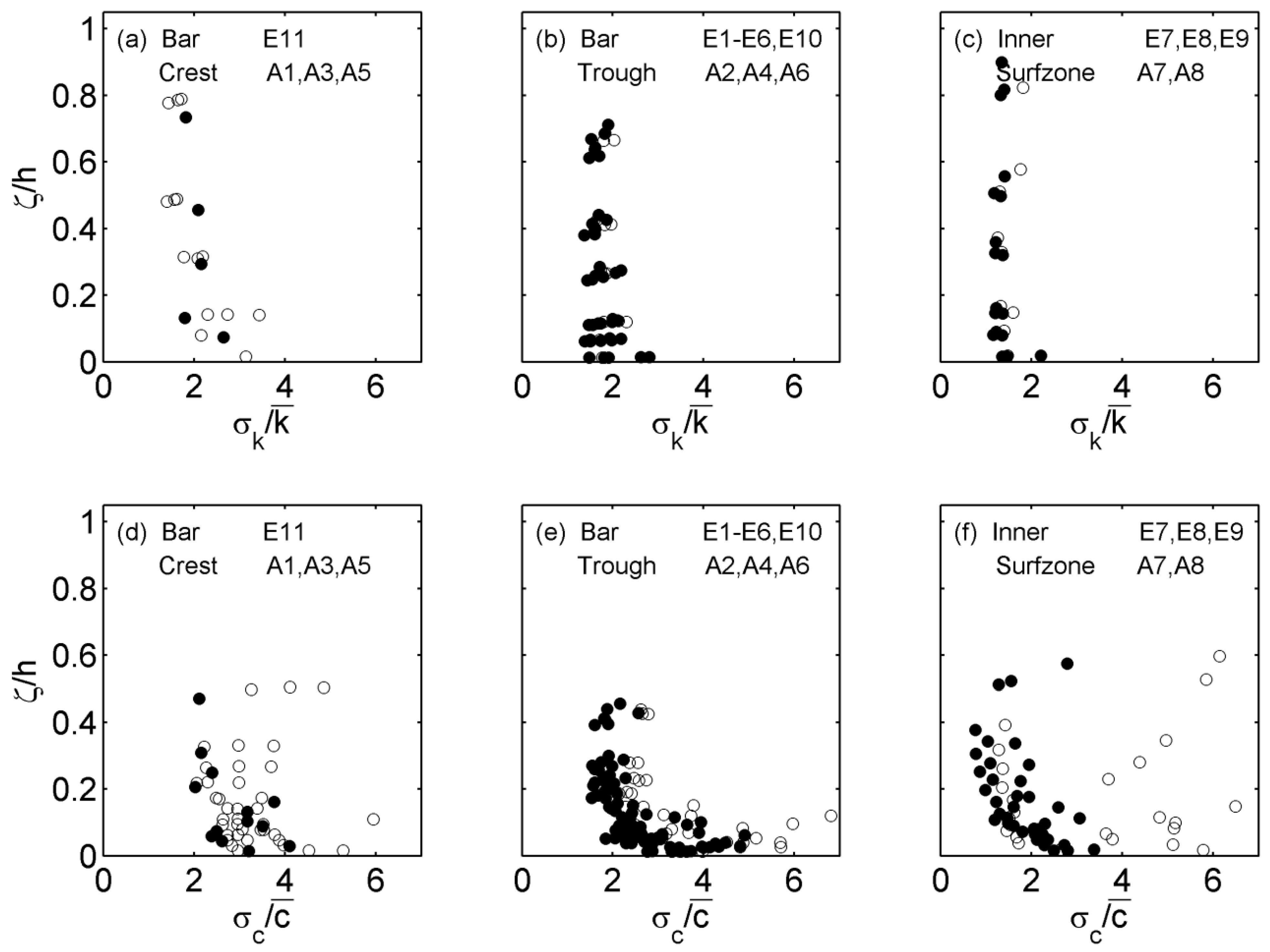
Figure 4 shows the vertical variation of the time-averaged TKE per unit mass ($\overline{k}$) and the time-averaged SSC ($\overline{c}$) across the surf zone, at the bar crest (E11 for erosive; A1, A3, and A5 for accretive), the bar trough (E1–E6 and E11 for erosive, A2, A4, and A6 for accretive), and the inner surf zone (E7–E9 for erosive; A7 and A8 for accretive). TKE and SSC were time-averaged from 100 s to 900 s. The upper panels (Figure 4a–c) show $\overline{k}$ for the erosive and accretive cases, normalized by the depth-averaged $\overline{k}$ (indicated by < $\overline{k}$ >) for each case. The vertical axis represents the relative elevation, where $\zeta$ is the elevation of a sensor from the bed and h is the water depth. Overall, it is somewhat striking that there is very little difference in the vertical profile of $\overline{k}$ between erosive and accretive conditions at each of the three location when normalized by < $\overline{k}$ > at each location. The value of < $\overline{k}$ > itself was consistent between erosive and accretive cases at the bar crest and increased by approximately 30% at the inner surf zone. Interestingly, at the bar trough, the value of < $\overline{k}$ > for the erosive is larger than that for accretive cases by 60%, compared to 10% variation over the bar and 4% in the inner surf zone. This large difference is difficult to explain in terms of $\overline{u}$ or $u_{rms}$ variations shown in Figure 2 and Figure 3, and highlights the complexity of shore-shore sediment transport in the surf zone.

Figure 4. Vertical variation of time-averaged turbulent kinetic energy per unit mass ($\overline{k}$) and suspended sediment concentration ($\overline{c}$) at bar crest (a,d); bar trough (b,e); and inner surf zone (c) and (f) for erosive (red) and accretive (blue) conditions. Values are normalized by the depth-averaged value from 0 < $\zeta /h$ < 0.5 and are indicated in angle brackets on each panel.

Figure 4. Vertical variation of time-averaged turbulent kinetic energy per unit mass ($\overline{k}$) and suspended sediment concentration ($\overline{c}$) at bar crest (a,d); bar trough (b,e); and inner surf zone (c) and (f) for erosive (red) and accretive (blue) conditions. Values are normalized by the depth-averaged value from 0 < $\zeta /h$ < 0.5 and are indicated in angle brackets on each panel.

The vertical distribution of $\overline{k}$ at the bar crest (Figure 4a) shows the largest variation over the depth. As most waves broke intensively at this location and impinged on the water surface, $\overline{k}$ was observed to be large near the water surface level but quickly decreased in the middle of the water column at approximately $\zeta /h$ = 0.3 and then was nearly uniform until the wave bottom boundary layer near the vicinity of the bed $\zeta /h$ = 0.1. One thing to note was that $\overline{k}$ increased slightly with depth in the vicinity of the bed ($\zeta /h$ <0.1) for both erosive and accretive conditions. Strong wave motions over shallow water depths at the bar crest may have generated bottom boundary turbulence and a shear motion, in addition to the wave breaking turbulence from the upper water column. At the bar trough (Figure 4b), $\overline{k}$ monotonically decreased downward without the reverse trend near the bottom that was observed in the bar crest. At the inner surf zone (Figure 4c), the vertical profile of $\overline{k}$ seems to fall, qualitatively, between the first two. That is, $\overline{k}$ near the upper is approximately 4 to 5 times larger than the bottom value, as was the case in Figure 4a at the bar crest. There is a distinct change in the vertical gradient of $\overline{k}$ at approximately $\zeta /h$ = 0.3, similar to Figure 4a. However, unlike Figure 4a, where the variation of $\overline{k}$ is almost uniform over depth with a slight increase in the vicinity of the bed, the variation of $\overline{k}$ decreases downward, consistent with the observations at the bar trough in Figure 4b.

The lower panels of Figure 4d–f illustrate the time-averaged SSC ($\overline{c}$). As with $\overline{k}$, the depth-averaged $\overline{c}$ is indicated as < $\overline{c}$ >. The magnitude of < $\overline{c}$ > is largest at the bar crest and trough, where the most intense and unsteady wave breaking occurs, and significantly decreases in the inner surf zone by almost a half. As expected, Figure 4d–f shows an increase in the $\overline{c}$ near the bed, but there are interesting similarities and differences between erosive and accretive concentration profiles at each of the regions. For example, Figure 4f in the inner surf zone shows that the normalized concentration profiles of both the erosive and accretive conditions shows vertically uniform profiles, except for the very close to the bottom. On the other hand, Figure 4e showed a strong difference in the profiles of $\overline{c}$/< $\overline{c}$ > between the erosive and accretive cases, despite of the nearly same profiles of $\overline{k}$/< $\overline{k}$ > in Figure 4b. In particular, the value of the normalized concentration near the bottom is about twice as large for the erosive case (red) compared to the accretive case (blue). This can be partly attributed to the 60% difference in < $\overline{k}$ >, but also be due to another sediment suspension mechanism such as adverse pressure gradient in the bar trough. Furthermore, Figure 4d,f show that the concentration profiles are nearly uniform over depth for $\zeta /h$ > 0.3 owing to the strong mixing by wave breaking. The data seem to suggest that the concentration profile is less uniform over the bar trough (Figure 4e) for the erosive case. Overall, there is an interesting similarity in the normalized turbulence and concentration profiles over the bar crest (Figure 4a,d) and the inner surf zone (Figure 4c,f) even though the values for normalization had opposite trends: < $\overline{k}$ > increased by 30% from bar to inner surf zone, but < $\overline{c}$ > decreased by a factor 2.

The intermittency of turbulence and sediment suspension can be examined using thresholds based on the mean and standard deviation of the observed $k$ and $c$ at each elevation (e.g., [15,25,26]). Yoon and Cox [15] observed that intermittent events of turbulent and suspension occurred for a small portion of the time series but contained a significant amount of motions in these events. The intermittent events were defined where the value of turbulent or sediment suspension exceed a certain threshold, such as a mean plus one standard deviation. Therefore the statistical parameters, such as mean and standard deviation, are important for understanding intermittent features of turbulent and sediment suspension. Figure 5 shows the statistical results such as the standard deviations of $k$ (${\mathrm{\sigma }}_k$) and $c$ (${\mathrm{\sigma }}_c$), normalized by $\overline{k}$ and $\overline{c}$, respectively, at each elevation. In some cases, ${\mathrm{\sigma }}_k$/$\overline{k}$ shows nearly uniform over the vertical as seen in Figure 5a–c for both erosive and accretive cases and is somewhat surprising given the vertical variation in $\overline{k}$ seen in Figure 4a–c. Overall, the value of ${\mathrm{\sigma }}_k$/$\overline{k}$ is approximately 2, although it appears to be slightly smaller for the inner surf zone. On the other hand, there seems to be a larger scatter in ${\mathrm{\sigma }}_c$/$\overline{c}$ as one might expect considering the characteristics of sediment concentration time series measured in the surf zone. Moreover, the vertical variation is no longer uniform over the vertical with ${\mathrm{\sigma }}_c$/$\overline{c}$ increasing near the bottom. For example, Figure 5e shows that ${\mathrm{\sigma }}_c$/$\overline{c}$ is approximately 2 for $\zeta /h$ > 0.1 and then increase downward by a factor of 2 to 3. One possible explanation for the larger ${\mathrm{\sigma }}_c$/$\overline{c}$ is the longer time scale for sediment suspension than for turbulence. Due to the shorter time scale, turbulence cannot be advected in the same way as suspended sediments are advected. Once sediments are suspended, they remain suspended for some time even after turbulence has dissipated. Also, some values of ${\mathrm{\sigma }}_c$/$\overline{c}$ for the accretive case were larger than that for the erosive case in the inner surf zone, and this is probably due to longer wave period, keeping sediments suspended longer.

Figure 5. Vertical variation of the ratio of the standard deviation (${\mathrm{\sigma }}_k$) to time-averaged turbulent kinetic energy per unit mass ($\overline{k}$) at the bar crest (a); bar trough (b) and inner surf zone (c) for erosive (closed dot) and accretive (open dot) conditions. Vertical variation of the same ratio for the suspended sediment concentration (${\mathrm{\sigma }}_c$/$\overline{c}$) at the same cross-shore locations (d–f).

Figure 5. Vertical variation of the ratio of the standard deviation (${\mathrm{\sigma }}_k$) to time-averaged turbulent kinetic energy per unit mass ($\overline{k}$) at the bar crest (a); bar trough (b) and inner surf zone (c) for erosive (closed dot) and accretive (open dot) conditions. Vertical variation of the same ratio for the suspended sediment concentration (${\mathrm{\sigma }}_c$/$\overline{c}$) at the same cross-shore locations (d–f).

4. Relation between Turbulent Kinetic Energy and Suspended Sediment Concentration

The understanding of the relationship between TKE and SSC is important for estimation and modeling of sediment transport in the surf zone. Based on the measurements obtained as described in the previous section, we propose the following simple relationship between $\overline{k}$ and $\overline{c}$ at the bar trough, bar crest, and inner surf zone.

$$\overline{c}(\zeta )=B\frac{{\overline{k}}^{3/2}}{\zeta /h}$$

(4)

where B is a dimensional coefficient (with units of $\frac{kg}{m^3}\cdot \frac{s^3}{m^3}$). The right-hand term in Equation (4) is analogous to the dissipation rate ($\epsilon$) in the typical $k-\epsilon$ equation, in which $\epsilon =C_D\frac{{\overline{k}}^{3/2}}{l}$ (e.g., [27]), where $C_D$ is an empirical constant (typically ~0.09) and l is the turbulent length scale. Traditionally, the length scale of turbulence in the surf zone is expressed as a function of the water depth, h, for example, l $\approx$ 0.2 h to 0.3 h ([28]), l $\approx$ 0.25 h ([29]), and l $\approx$ 0.1 h to 0.2 h ([30]), and is considered to be vertically uniform. Pedersen et al. [31] argued that the turbulent length scale is not uniform but rather decreases linearly in the vicinity of the bed, varying in the range of $l\approx 0.15$~0.3 h below $\zeta /h$ < 0.15.

Especially, Cox et al. [32] noted that l also varied from 0.04 h (outside surf zone) to 0.18 h (inner surf zone) according to the cross-shore locations. In the present study, it is assumed that $\overline{c}$is proportional to the turbulent dissipation rate at a specific elevation. The turbulent length scale is also assumed to be dependent on the elevation above the bed and to be expressed in a dimensionless form as $l=\zeta /h$. According to these assumptions, the length scale decreases downward because of the effect of the bottom and the contribution of turbulent dissipation to $\overline{c}$ increases downward. In the following, we investigated the relationship between $\overline{k}$ and $\overline{c}$ experimentally by examining the coefficient B in Equation (4) and the R² (coefficient of determination) values at the characteristic locations of the barred beach, i.e., the bar crest, trough, and inner surf zone.

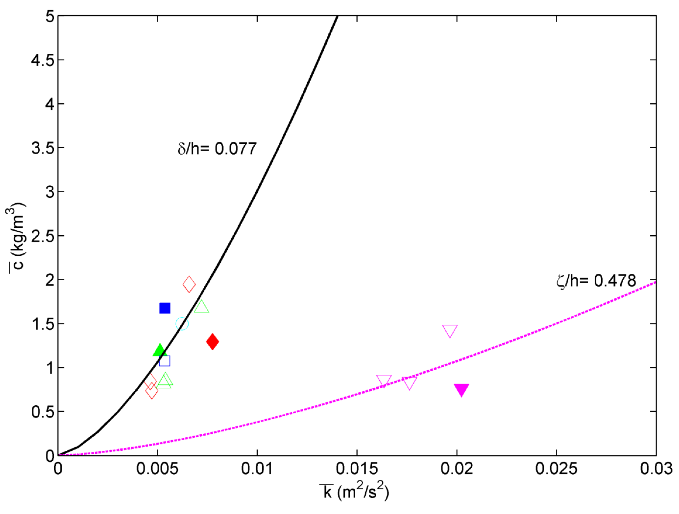
At the bar crest, the relationship between $\overline{k}$ and $\overline{c}$ was weak at elevations within ~20 cm above the bed ($\zeta /h$ ~ 0.3). This is shown in Figure 6 in which the relation between $\overline{k}$ and $\overline{c}$ measured at the bar crest for erosive conditions E11 (solid markers) and accretive conditions A1, A3, and A5 (open markers). For the cases in the range of 1 cm ≤ $\zeta$ ≤ 20 cm (0.016 ≤ $\zeta /h$ ≤ 0.309), $\overline{c}$ was correlated to neither $\overline{k}$ nor elevation, exhibiting a cluster of data points. Also, there was no clear difference in the turbulence magnitude between the erosive and accretive cases. The bar crest is the region in which depth-limited wave breaking occurs primarily and most strongly over shallow water depths. Thus, sediment could be strongly suspended and mixed farther away from the bed. In addition, strong wave-induced motion in shallow water depths (see Figure 2 and Figure 3) can enhance sediment suspension and mixing with current shear. Therefore, for the bar crest case, we modified Equation (4) slightly as follows:

$$\overline{c}(\zeta )=B\frac{{\overline{k}}^{3/2}}{\delta /h}$$

(5)

where $\delta$ is the wave bottom boundary layer thickness (~5 cm), which is taken as a reasonable first estimate for the mixing length near the bottom [33]. The black solid line in Figure 6 represents the fitted curve (Equation (5)) for elevations of 1 cm ≤ $\zeta$ ≤ 20 cm (0.016 ≤ $\zeta /h$ ≤ 0.309) and showed reasonable results with R² = 0.66 considering the complexity of sediment suspension mechanism in the surf zone. When we applied Equation (4) to the case of $\zeta /h$ = 0.478, which is in the middle of water column, the least-square fit with Equation (4) yields B = 180 with scattered data (R² = 0.04), as shown in Table 1.

Figure 6. Relation between time-averaged turbulent kinetic energy ($\overline{k}$) and suspended sediment concentration ($\overline{c}$) over the bar crest for erosive condition E11 (solid markers) and accretive conditions A1, A3, and A5 (open markers), classified by depth: $\zeta /h$ = 0.016 (cyan circles), 0.079 (blue squares), 0.139 (red diamonds), 0.309 (green triangles), and 0.478 (magenta triangles pointing downward). The solid black line indicates the least-square best fit to Equation (5) for B = 230 (R² = 0.66) and $\delta /h$ = 0.077, where $\delta$ is the bottom boundary layer thickness (~5 cm). The dashed line indicates the best fit to Equation (4) for $\zeta /h$ = 0.478.

Figure 6. Relation between time-averaged turbulent kinetic energy ($\overline{k}$) and suspended sediment concentration ($\overline{c}$) over the bar crest for erosive condition E11 (solid markers) and accretive conditions A1, A3, and A5 (open markers), classified by depth: $\zeta /h$ = 0.016 (cyan circles), 0.079 (blue squares), 0.139 (red diamonds), 0.309 (green triangles), and 0.478 (magenta triangles pointing downward). The solid black line indicates the least-square best fit to Equation (5) for B = 230 (R² = 0.66) and $\delta /h$ = 0.077, where $\delta$ is the bottom boundary layer thickness (~5 cm). The dashed line indicates the best fit to Equation (4) for $\zeta /h$ = 0.478.

Table 1. Coefficient B in Equation (5) and R² at bar crest.

ζ (cm) or δ (cm)	$\zeta /h$ or $\delta /h$	B	R2
5.0 (δ)	0.077	230	0.66
31.0 (ζ)	0.478	180	0.04

Table 1. Coefficient B in Equation (5) and R² at bar crest.

ζ (cm) or δ (cm)	$\zeta /h$ or $\delta /h$	B	R2
5.0 (δ)	0.077	230	0.66
31.0 (ζ)	0.478	180	0.04

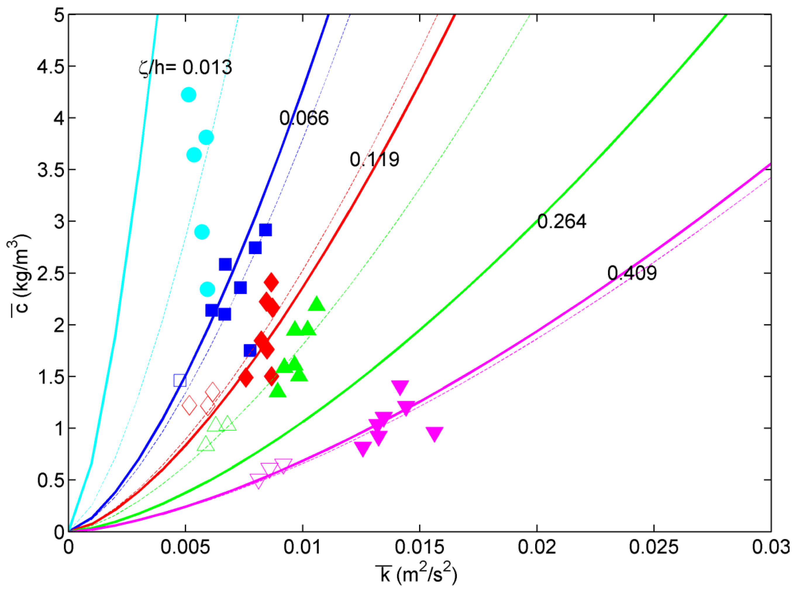
Next, we examined the case at the bar trough where the transient motion is predominant after the initial wave breaking over the bar crest as noted in Yoon and Cox [15]. Figure 7 shows the relation between $\overline{k}$ and $\overline{c}$ measured at the bar trough for erosive conditions E1–E6 and E10 (solid markers) and accretive conditions A2, A4, and A6 (open markers). The turbulent intensity ($\overline{k}$) for the erosive case is larger than that for accretive case because of stronger wave breaking conditions. The solid lines in Figure 7 indicate the “global” best fit to Equation (4) for B = 280 (R² = 0.72), for all of the data at the elevations of $\zeta /h$ = 0.013, 0.066, 0.119, 0.264 and 0.409 (see Table 2). The tuning parameter B, which accounts for the physics of the sediment suspension mechanism besides $\overline{k}$ and $\zeta /h$, appears to be suitable for use in determining the relationship. The fitting results suggest that $\overline{c}$ could be simply parameterized by the turbulent flow using Equation (4) which is similar to the equation for the turbulent dissipation rate. However, there were some discrepancies at $\zeta /h$ = 0.013 and 0.264 when we applied the “global” fit to all of the elevations.

Figure 7. Relation between time-averaged turbulent kinetic energy ($\overline{k}$) and suspended sediment concentration ($\overline{c}$) over the bar trough for erosive conditions E1–E6 and E10 (solid markers) and accretive conditions A2, A4, and A6 (open markers) classified by depth: $\zeta /h$ = 0.013 (cyan circles), 0.066 (blue squares), 0.119 (red diamonds), 0.264 (green triangles), and 0.409 (magenta triangles pointing downward). Solid lines indicate the least-square best fit to Equation (4) for B = 280 (R² = 0.72) for elevations $\zeta /h$ = 0.066, 0.119, 0.264, and 0.409, except for $\zeta /h$ = 0.013. Dashed lines indicates the best fit to Equation (4) for B determined for each elevation.

Figure 7. Relation between time-averaged turbulent kinetic energy ($\overline{k}$) and suspended sediment concentration ($\overline{c}$) over the bar trough for erosive conditions E1–E6 and E10 (solid markers) and accretive conditions A2, A4, and A6 (open markers) classified by depth: $\zeta /h$ = 0.013 (cyan circles), 0.066 (blue squares), 0.119 (red diamonds), 0.264 (green triangles), and 0.409 (magenta triangles pointing downward). Solid lines indicate the least-square best fit to Equation (4) for B = 280 (R² = 0.72) for elevations $\zeta /h$ = 0.066, 0.119, 0.264, and 0.409, except for $\zeta /h$ = 0.013. Dashed lines indicates the best fit to Equation (4) for B determined for each elevation.

Table 2. Coefficient B in Equation (4) and R² at bar trough.

ζ (cm)	$\zeta /h$	B	R2
1.0	0.013	530	0.23
5.0	0.066	250	0.69
9.0	0.119	300	0.72
20.0	0.264	480	0.90
31.0	0.409	270	0.77
Global (ζ = 5.0–31.0)		280	0.72

Table 2. Coefficient B in Equation (4) and R² at bar trough.

ζ (cm)	$\zeta /h$	B	R2
1.0	0.013	530	0.23
5.0	0.066	250	0.69
9.0	0.119	300	0.72
20.0	0.264	480	0.90
31.0	0.409	270	0.77
Global (ζ = 5.0–31.0)		280	0.72

When we applied Equation (4) to each elevation separately, we were able to obtain better agreement between $\overline{c}$ and $\overline{k}$. The dashed lines in Figure 7 indicate the “local” best fit to Equation (4) for B determined for each elevation. The “local” best fit yielded better agreement than the “global” fit above the bottom boundary layer ($\zeta$ ≥ 9 cm or $\zeta /h$ ≥ 0.119), as shown in Table 2. The relationship between $\overline{k}$ and $\overline{c}$ had R² ≥ 0.72 with B = 270–480 (average: 350) for the elevations $\zeta /h$ ≥ 0.119. This confirms that SSC is closely related to turbulent flow and can be parameterized using Equation (4) if the intensity of breaking wave (or turbulent intensity) is enough large such as at the bar trough. However, even the “local” fit achieved is not good close to the bottom, as seen in the case of $\zeta /h$ = 0.013 where R² = 0.23. The proposed relationship yielded good agreement only above the wave bottom boundary layer, which may be because another suspension mechanism (e.g., sheet flow) is predominant close to the bottom except near the bar trough.

At the inner surf zone, the relationship between $\overline{k}$ and $\overline{c}$ is not as strong. $\overline{k}$ and $\overline{c}$ for the erosive and accretive cases exhibited no clear difference, as was the case of the bar crest. Here, Equation (4) fits reasonably well near the bottom (within 5 cm above the bed), with R² values in the range of 0.44 to 0.49. Note that the coefficient of B in Equation (4) is smaller than at the other locations by almost an order of magnitude, because the suspended sediment concentration is lower in the inner surf zone than at the other locations. At elevations greater than 5 cm above the bed, the agreement rapidly decreases and R² approaches zero.

5. Summary and Conclusions

The relationship between the time-averaged turbulent kinetic energy per unit mass and the sediment concentration was examined at the bar crest, trough, and inner surf zone of a beach using data from a large-scale laboratory experiment. For both erosive and accretive bathymetric conditions, the time-averaged sediment concentration was tentatively parameterized using Equation (4), which is analogous to the equation for the turbulent dissipation rate. For the bar crest location, where strong wave breaking motion coexists with wave motions near the bottom, we modified Equation (4) and suggested Equation (5), replacing the turbulent length scale with the wave bottom boundary layer thickness. Equation (5) describes the relationship between the time-averaged turbulent kinetic energy and the sediment concentration near the bottom, which suggests that the mixing length scale at the bar crest is rather related to the bottom boundary layer thickness. At the bar trough, where wave breaking turbulence tends to maintain sediment suspension, this relationship shows the best fit to the experimental data, except for the region very close to the bed. For the inner surf zone, however, Equation (4) does not show a good agreement with the experimental data as seen in other region. These results imply that different sediment suspension mechanisms predominate in the inner surf zone. Overall, although there are other mechanisms that affect the sediment suspension in the surf zone, the time-averaged SSC can be parameterized with the TKE. These findings can be used to better quantify and model the effect of turbulence on sediment suspension in the surf zone.