The Characteristics and Contributing Factors of Air Pollution in Nanjing: A Case Study Based on an Unmanned Aerial Vehicle Experiment and Multiple Datasets

Abstract

Unmanned aerial vehicle (UAV) experiments, multiple datasets from ground-based stations and satellite remote sensing platforms, and backward trajectory models were combined to investigate the characteristics and influential mechanisms of the air pollution episode that occurred in Nanjing during 3–4 December 2017. Before the experiments, the position of the detector mounted on a UAV that was minimally disturbed by the rotation of the rotors was analyzed based on computational fluid dynamics (CFD) simulations. The combined analysis indicated that the surface meteorological conditions—high relative humidity, low wind speed, and low temperature—were conducive to the accumulation of PM_2.5. Strongly intense temperature inversion layers and the low thickness of the atmospheric mixed layer could have resulted in elevated PM_2.5 mass concentrations. In the early stage, air pollution was affected by the synoptic circulation of the homogenous pressure field and low wind speeds, and the pollutants mainly originated from emissions from surrounding areas. The aggravated pollution was mainly attributed to the cold front and strong northwesterly winds above 850 hPa, and the pollutants mostly originated from the long-distance transport of emissions with northwesterly winds, mainly from the Beijing‒Tianjin‒Hebei (BTH) region and its surrounding areas. This long-distance transport predominated during this event. The air pollution level and aerosol optical depth (AOD) were positively correlated with respect to their spatial distributions; they could reflect shifts in areas of serious pollution. Pollution was concentrated in Anhui Province when it was alleviated in Nanjing. Polluted dust, polluted continental and smoke aerosols were primarily observed during this process. In particular, polluted dust aerosols accounted for a major part of the transport stage, and existed between the surface and 4 km. Moreover, the average extinction coefficient at lower altitudes (<1 km) was higher for aerosol deposition.

1. Introduction

With the recent social modernization and industrialization coincident with the rapid increase in energy consumption and the intense emissions of air pollutants, major cities throughout China have frequently suffered from serious regional air pollution. Air pollution, which is characterized by the deterioration of the air quality and the degradation of visibility [1,2,3], not only significantly influences the urban environment and traffic safety but also poses a substantial threat to human health by causing diseases such as pneumonia, bronchitis, and cardiovascular disease [4,5,6,7]. In the long run, air pollution leads to changes in aerosol optical properties and the radiation budget of the earth-atmosphere system, thereby influencing the climate [8,9]. Therefore, the frequent occurrence of air pollution episodes in China has become a scientific issue and aroused great public concern.

Air pollution events are essentially subject to the impacts of emission sources and regional transport characteristics in addition to the atmospheric diffusion capacity [10], which is primarily related to meteorological conditions and synoptic situations. The characteristics and causes of air pollution episodes, such as haze pollution, have been widely analyzed in many studies based on observations, measurements, and numerical calculations, the results of which could provide a theoretical basis for the prevention and effective emergency warning of pollution events and the reduction in emissions. Research suggests that the accumulation, transport, and dissipation of pollutants are affected by meteorological elements, including wind speed, temperature, relative humidity, and precipitation [11,12]. However, the primary elements may affect the evolution and intensity of pollution in a variable way due to geographical differences [13]. Furthermore, the presence of stable atmospheric stratification and the evolution of proper circulations are also important influencing factors on the variation in pollutants with respect to their spatial and temporal distributions [14,15,16]. In addition, long-term strong temperature inversion layers and lower atmospheric mixed layer height could contribute to the inhibition of diffusion conditions, resulting in continuous accumulation of pollutants [17].

Real-time monitoring of the vertical spatial distribution of meteorological elements in the atmospheric boundary layer is another important factor that should be taken into consideration. Although many studies have been performed to investigate the effects of the meteorological conditions within the atmospheric boundary layer on the formation, maintenance and dissipation of air pollution episodes, the results were generally based on conventional methods using manned aircraft, sounding balloons, and tethered airships. These methods are characterized by high cost and poor maneuverability. In contrast, the use of unmanned aerial vehicles (UAVs) carrying sensors or other detection equipment to sample data in the atmospheric boundary layer presents numerous distinct advantages and has rapidly increased in the field of atmospheric research [18]. First, it can greatly reduce operational costs and perform measurements at any time due to the portability of UAVs. Second, it can increase the density of sampling data and collect more substantial data than fixed-point observation techniques, providing a more effective determination of the characteristics of pollutant transport and the key factors during the pollution process [19,20,21]. Based on these advantages, the positions of detectors mounted on UAVs have been discussed with regard to the disturbances generated by the rotation of rotors. In addition, some researchers have also focused on barriers to successful unmanned technology adoption, including system selection, tactical deployment, training, and dealing with the rapid evolution of technology and regulations [22].

Due to the limitations on the spatial coverage and frequency of observations for sampling data, measurements by satellite remote sensing technology have achieved impressive progress in weather monitoring. Many studies have been performed to investigate aerosol optical properties with the convenient acquisition of aerosol parameters. At present, there are two main analysis methods for air pollution processes: analyzing the regional aerosol optical properties [23] and analyzing the vertical distribution characteristics of aerosols [24,25]. Moreover, because the observations from remote sensing platforms are closely related to shifts in the regions of air pollution, these investigations could also provide evidence to support the prevention of air pollution.

Nanjing, the capital city of Jiangsu Province, is an important central city in eastern China, and it has suffered from frequent air pollution events in recent years. A pollution episode was observed in Nanjing during 3–4 December 2017. Accordingly, this study aims to analyze the characteristics and contributing factors of air pollution, including the meteorological conditions, potential mechanisms for increases in pollutants, and aerosol properties. In addition, the use of UAVs to conduct measurements for this work could provide a reference for the development of UAVs in monitoring and forecasting air pollution episodes. Various data from ground-based stations and satellite remote sensing platforms were introduced to analyze this event. Section 2 presents the proper positions for detection equipment mounted on UAVs that are disturbed relatively little by the flow field. Section 3 introduces the UAV experiment and the adopted data and methods for the analysis. The results are analyzed in Section 4. The discussion and conclusions are given in Section 5.

2. UAV Platform and Flow Field Simulation

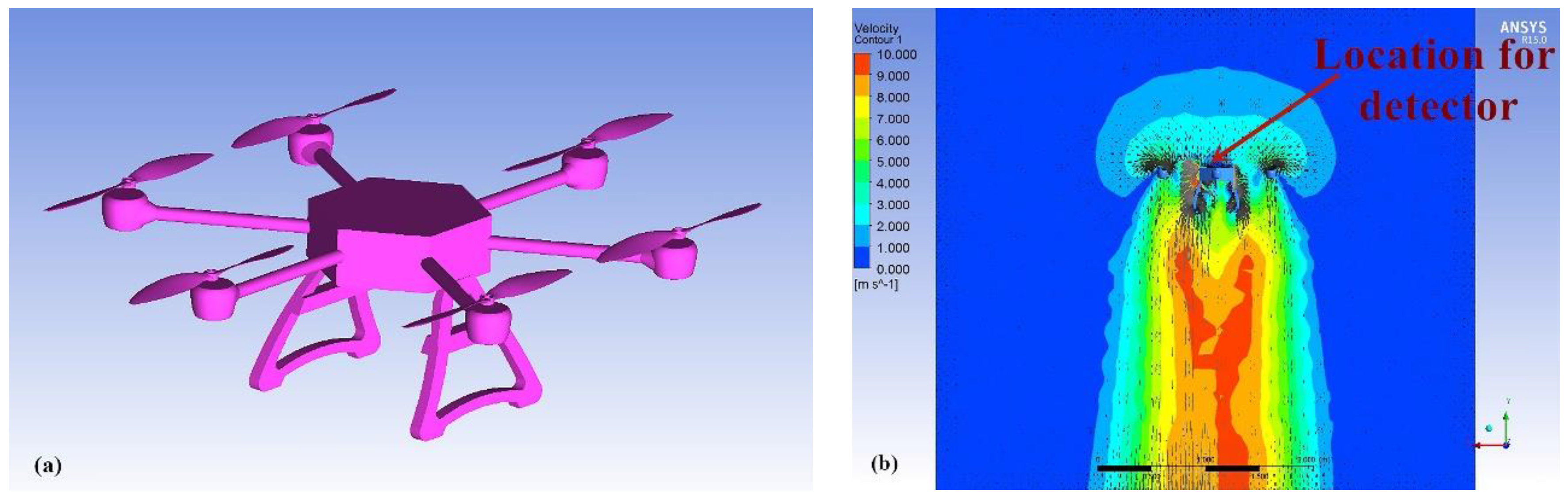
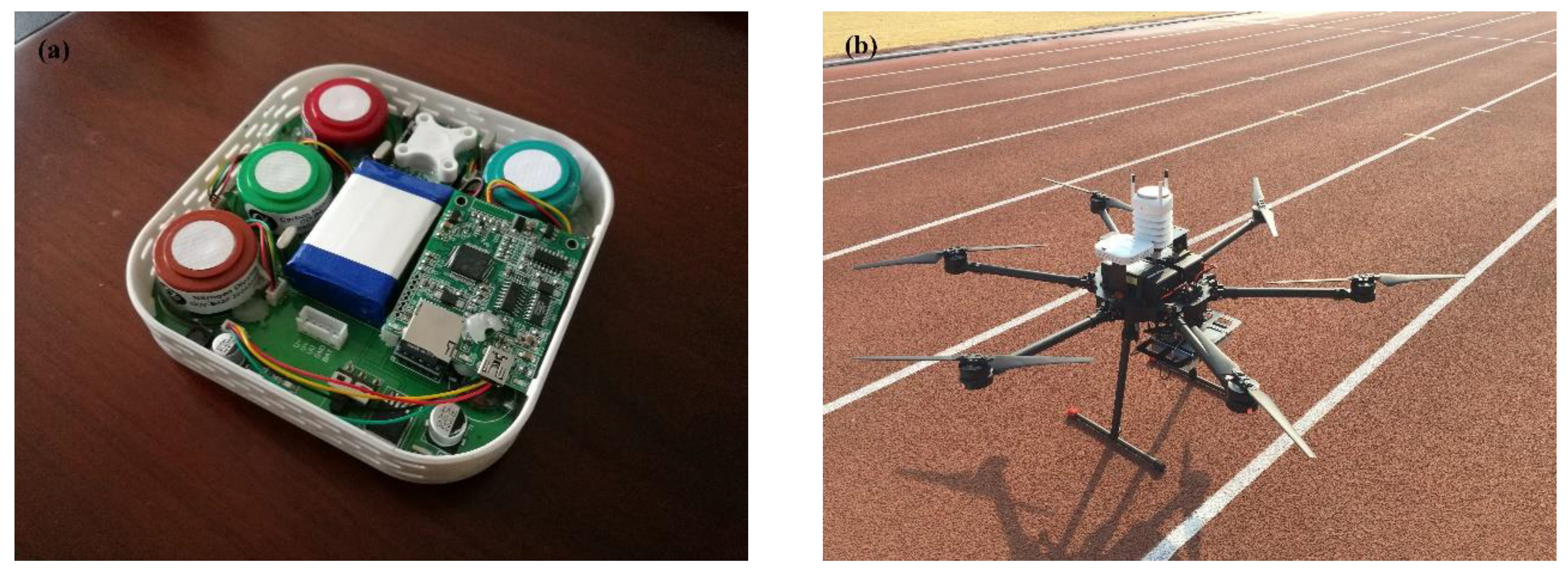
The vertical measurement for distribution of meteorological elements and pollutant concentration in the atmospheric boundary layer has the important scientific significance, including fully recognizing the comprehensive characteristics of air pollution process and providing the optimal strategy for the prevention and control of air pollution. Conventional methods (i.e., meteorological observation tower, sounding balloons, and tethered airships) for monitoring the vertical spatial distribution of meteorological and pollutant elements present many shortcomings. Among them, lack of obtaining the three-dimensional synchronous data in the atmospheric boundary layer cannot fully meet the needs of current theoretical research and business application. The use of UAV carrying detection equipment could obtain data at different spatial locations flexibly according to the characteristics of air pollution process. In addition, it has the advantages of low cost, fix-point hovering, and low requirement for take-off and landing techniques, which could remedy the lack of conventional measuring. Obviously, this detection method is an important supplement to existing detection technology.

With the use of UAV platform, the position of detectors mounted on UAV should be discussed. The disturbance of the air flow field caused by the rotors of the UAV could lead to obvious deviations in the measurements, particularly because some elements in the detection equipment could be affected by the flow field in the aspect of heat dissipation and particle sampling. Consequently, the positions of detection equipment on UAVs at which they are scarcely disturbed by disturbances in the air flow field should be taken into consideration.

2.1. Platform

The UAV platform applied for the data acquisition is the CEEWA X8 (Nanjing CEEWA Intelligent Technology Co., Ltd., Nanjing, China), a six-rotor industrial UAV carrying highly reliable, triple-redundant FC-IU3 flight control system. This platform can work with portable ground stations, being easy to use and operationally flexible. The CEEWA X8 weighs 13.5 kg, the payload is 5.5 kg, and the rotor radius is 266 mm. Its relatively heavy airframe and long rotors result in a smooth flight, which offers good resistance to wind shear. The battery provides 55 min for flight under certain weather conditions. The CEEWA X8 receives control signals from a ground station through wireless communication and achieves automatic flight with its own self-driving instrument.

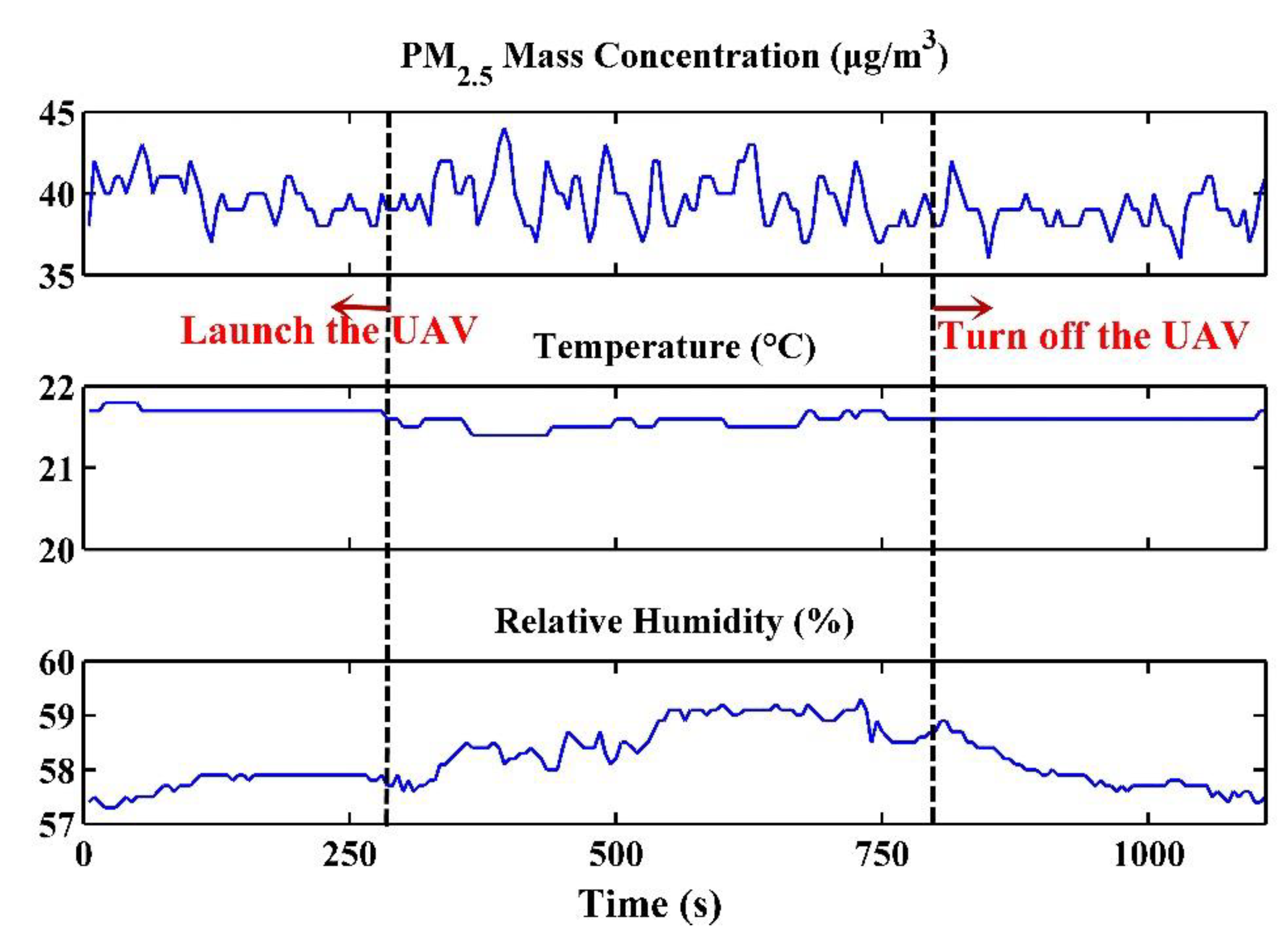
2.2. Flow Field Simulation of UAV

The computational fluid dynamics (CFD) simulation technique, which can effectively simulate the flow field, is adopted to determine the most reliable position for the placement of a detector.

In general, the laws of the conservation of mass, momentum, and energy are used to calculate the flow field through CFD simulation. In addition, the turbulence model should be added because the unknown quantity known as the Reynolds strain item produced in the momentum equations results in unclosed equations. To close the equations, the standard k‒ε turbulence model is applied to the numerical calculation to simulate the flow field because of its extensive use, high efficiency, and reasonable precision [26,27]. The equation for the turbulent kinetic energy dissipation ratio (ε) is introduced on the basis of the turbulent kinetic energy (k) equation, forming the k‒ε equations [28]:

$$\frac{\partial \left(\rho k\right)}{\partial t}+\frac{\partial \left(\rho k{u}_i\right)}{\partial x_i}=\frac{\partial }{\partial x_j}\left[\left(\mu +\frac{{\mu }_t}{{\sigma }_k}\right)\frac{\partial k}{\partial x_j}\right]+G_k+G_b-\rho \epsilon -Y_M+S_k$$

(1)

$$\frac{\partial \left(\rho \epsilon \right)}{\partial t}+\frac{\partial \left(\rho \epsilon u_i\right)}{\partial x_i}=\frac{\partial }{\partial x_j}\left[\left(\mu +\frac{{\mu }_t}{{\sigma }_{\epsilon }}\right)\frac{\partial \epsilon }{\partial x_j}\right]+G_{1\epsilon }\frac{\epsilon }{k}\left(G_k+C_{3\epsilon }{G}_b\right)-C_{2\epsilon }\rho \frac{{\epsilon }^2}{k}+S_{\epsilon }$$

(2)

where G_k and G_b are the turbulent kinetic energy components produced by the average velocity gradient and buoyancy, respectively, and Y_m is the influence of compressible turbulence on the total dissipative rate. C_1ε, C_2ε and C_3ε are the empirical constants, the values of which are 1.44, 1.92 and 0.09, respectively. σ_k and σ_ε are the Prandlt numbers corresponding to k and ε, respectively, the default values of which are 1.0 and 1.3. S_k and S_ε are the source terms.

Based on the model selected above, the flow field simulation of a UAV in a hover state is as follows. (1) Model the six-rotor UAV (Figure 1a). The airframe and the brackets are simplified because the model is mainly used to analyze the influence of the airflow generated by the rotors. (2) Select the calculation region and generate the grid. The grids around the rotor are refined, while the rest of the grids are relatively sparse considering the accuracy and efficiency of the calculation. (3) Set the boundary conditions. The fan boundary condition is applied to approximately describe the rotors by defining the pressure difference above and below the rotors during high-speed rotation of the UAV. (4) Obtain the calculation result.

Note that the UAV is used to sample data at each altitude in a hover state. Thus, the flow field of the six-rotor UAV in a hover state is shown in Figure 1b. The velocity below the UAV is distinctly strong. In contrast, the velocity above the airframe is relatively weak and thus represents the position less influenced by the airflow generated by the rotation of the rotors. Therefore, in consideration of a greater measurement accuracy and less interference, the detector can be placed above the airframe, and its position is indicated by the red arrow in Figure 1b.

3. Methodology

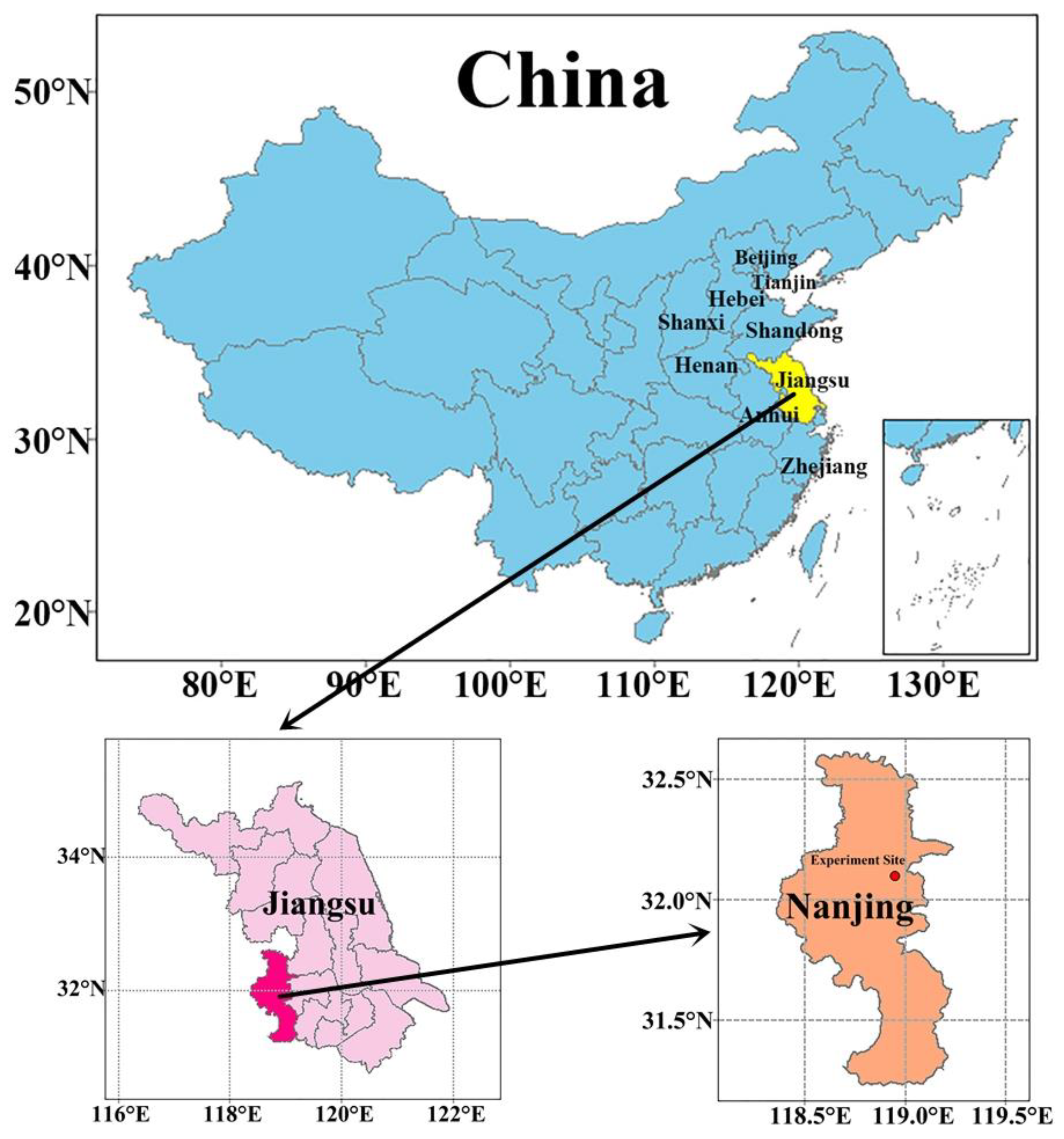
3.1. Experiment Overview

The experiment was performed on the Xianlin campus of Nanjing University in the eastern suburb of Nanjing (32°06’ N, 118°57’ E), the capital of Jiangsu Province, which is surrounded by farmland, residential areas, and small patches of forest and chemical plants (Figure 2). The site was located on a playground, a flat location that was not surrounded by tall structures.

Figure 3a shows the detection equipment mounted on the UAV used to monitor the meteorological variables and PM_2.5 levels. PM_2.5 refers to fine particulate matter, which contributes greatly to air pollution, such as haze pollution. The UAV was equipped with a multiparameter atmospheric environment detector developed by Shenzhen TENGWEI Measurement and Control Technology Co., Ltd., Shenzhen, China. The detector weighs 350 g, and the battery life reaches up to 360 min. The detector integrates temperature, relative humidity, height and PM_2.5 mass concentration sensors, a main control board, a rechargeable battery and a data storage module. The main control board collects data in coordination with the sensors, and the data, which can be downloaded through a USB port, are stored in the storage module every 5 s. The temperature sensor is a thermistor-type probe, and its measurement accuracy is ±0.3 °C. The relative humidity sensor is a hygristor with an accuracy of ±3%. The PM_2.5 mass concentration sensor acquires data by analyzing the photoelectric characteristics of the samples on the basis of the laser principle. Air intake and outlet are included in this sensor to sample the air. During the sampling process, the light scattering occurs when the laser is used to irradiate the particulate matters suspended in the sampled air. The scattered light is collected at a certain angle, and thus, we can obtain the temporal variation of the scattering intensity. Then, the algorithm based on scattering theory is combined in the microprocessor to calculate the mass of the particulate matters per unit volume in the sampled air. Its accuracy is ±10 μg/m³. The detector is installed above the airframe of the UAV platform (Figure 3b) to minimize the interference from the airflow caused by the rotation of the rotors, as discussed above, and Appendix A also presents the experiment results about the validity of detector’s position on UAV. Combined with the detection equipment and batteries that provide power to the UAV during the flight, the total weight for the flight experiment is approximately 16.5 kg.

The flights took place over two days during 3–4 December 2017 at the above experiment site, and were carried out every three hours beginning at approximately 09:00 local standard time (LST) on 3 December, as outlined in

Table 1. Flight information. The takeoff time refers to the local standard time (UTC+8).

Flight ID	Takeoff Time	Flight ID	Take off Time	Flight ID	Takeoff Time
A1	09:00 LST 3 December	B1	21:00 LST 3 December	C1	09:00 LST 4 December
A2	12:00 LST 3 December	B2	00:00 LST 4 December	C2	12:00 LST 4 December
A3	15:00 LST 3 December	B3	03:00 LST 4 December	C3	15:00 LST 4 December
A4	18:00 LST 3 December	B4	06:00 LST 4 December	C4	18:00 LST 4 December

. The three groups, i.e., A, B, and C, represented the daytime of 3 December, from the evening of 3 December to the early morning of 4 December, and the daytime of 4 December, respectively. Each flight lasted approximately 20 min, and data were collected between the surface and 1000 m above ground level (AGL). During flight, the UAV climbed directly to the altitude of 1000 m AGL and hovered at altitudes of 1000, 900, 800, 700, 600, 500, 250 and 100 m AGL in the same vertical direction for approximately 2 min to acquire data on the above altitudes with greater reliability during its falling stage. The method of data sampled in the falling stage was adopted mostly because the sufficient voltage is needed to support for the UAV during the rising stage. However, the voltage of lithium battery would gradually decrease under working conditions, and the lower voltage would not support the UAV to continue rising. So, it is more appropriate to carry out measurements at each altitude in the UAV hover state during the falling stage. In addition, after some test flights, we compared the data sampled in UAV hover state during rising and falling stages, and the difference at each altitude between the two types was very small after eliminating outliers, which proved the feasibility of the scheme. Among the measurements, outliers could be generated by the unstable airflow when the UAV changed from a descending state to hovering state. In addition, the measurement deviations may also come from the detector itself. Therefore, to improve precision, outliers were eliminated, and the average values of continuous reliable measurements at each altitude in a hover state were calculated. We also obtained the vertical profiles of each parameter (i.e., the air temperature, relative humidity, and PM_2.5 mass concentration).

3.2. Data Collection and Methods

(1) The air quality index (AQI) and surface concentrations of particulate matter (PM_2.5 and PM₁₀) were recorded every hour at the Xianlin University Town monitoring site in Nanjing (32°06’ N, 118°54’ E), which is one of the China National Environmental Monitoring Center stations in Nanjing. Based on the National Ambient Air Quality Standards of China (NAAQS-2012), the air quality levels are divided into six levels according to the AQI such that the pollution level increases with an increase in the AQI. AQI values falling in the ranges of 0–50, 51–100, 101–150, 151–200, 201–300 and larger than 300 correspond to air quality levels of excellent, good, lightly polluted, moderately polluted, heavily polluted, and severely polluted levels, respectively [13,29].

(2) To reveal the evolution of the synoptic situation during the pollution episode, the National Centers for Environmental Prediction (NCEP) Final (FNL) operational global analysis data with a resolution of 1° × 1° and the European Center for Medium-Range Weather Forecasts (ECMWF) reanalysis data with a resolution of 0.125° × 0.125° were obtained. In addition, surface meteorological data, including the temperature, relative humidity, wind speed, and direction, were obtained from the regional automatic weather station in the Xianlin area of Nanjing.

(3) For the analysis of the potential source areas and transport paths of the pollutants, the Hybrid Single Particle Lagrangian Integrated Trajectory (HYSPLIT) model was used to calculate the backward trajectories of air masses [23]. In addition, the model developed by the National Oceanic and Atmospheric Administration (NOAA) was run in combination with meteorological data from the Global Data Assimilation System (GADS).

(4) The thickness of the atmospheric mixed layer is an important parameter for expressing the thermodynamic and dynamic characteristics of the atmospheric boundary layer; it characterizes the heights that pollutants can reach in the vertical direction through thermal convection and dynamic turbulent transport, thereby reflecting the extent of pollutant dissipation. In this work, the method proposed by Nozaki [30] in 1973 was applied to calculate the mixed layer thickness as follows:

$$H=\left(\frac{121}{6}\right)\left(6-P\right)\left(T-T_d\right)+\frac{0.169P\left(U_z+0.257\right)}{12f\ln \left(Z/Z_0\right)},$$

(3)

where P is the Pasquill stability level, which is divided into six levels ranging from A to F corresponding to the values from one to six. T − T_d is the dew-point deficit (°C). U_z is the average wind speed at 10 m AGL (m/s). f is the geostrophic parameter (s⁻¹). Z refers to an altitude of 10 m AGL. Z₀ is the surface roughness, the value of which is one in this work [13].

(5) The aerosol optical depth (AOD) product from the Moderate Resolution Imaging Spectroradiometer (MODIS) mounted on the Aqua satellite was used for the analysis of the evolution and characteristics of the spatial distribution of aerosols during the pollution episode. The AOD data at 550 nm were obtained from the MYD04_3K product with a resolution of 3 km × 3 km.

To analyze the vertical distribution characteristics of aerosols, aerosol products from the Cloud-Aerosol Lidar with Orthogonal Polarization (CALIOP) instrument mounted on the Cloud-Aerosol Lidar and Infrared Pathfinder Satellite Observation (CALIPSO) satellite were applied. We used the Level 2 products of the aerosol types and extinction coefficient at 532 nm. The aerosol types were divided into six categories: clean marine, dust, polluted continental, clean continental, polluted dust, and smoke aerosols. In addition, the extinction coefficient in Level 2 profile products is acquired based on the Level 1 products. Due to the errors resulting in the inaccuracy of Level 2 products in the algorithm, the data quality control method should be adopted [31,32,33].

4. Results

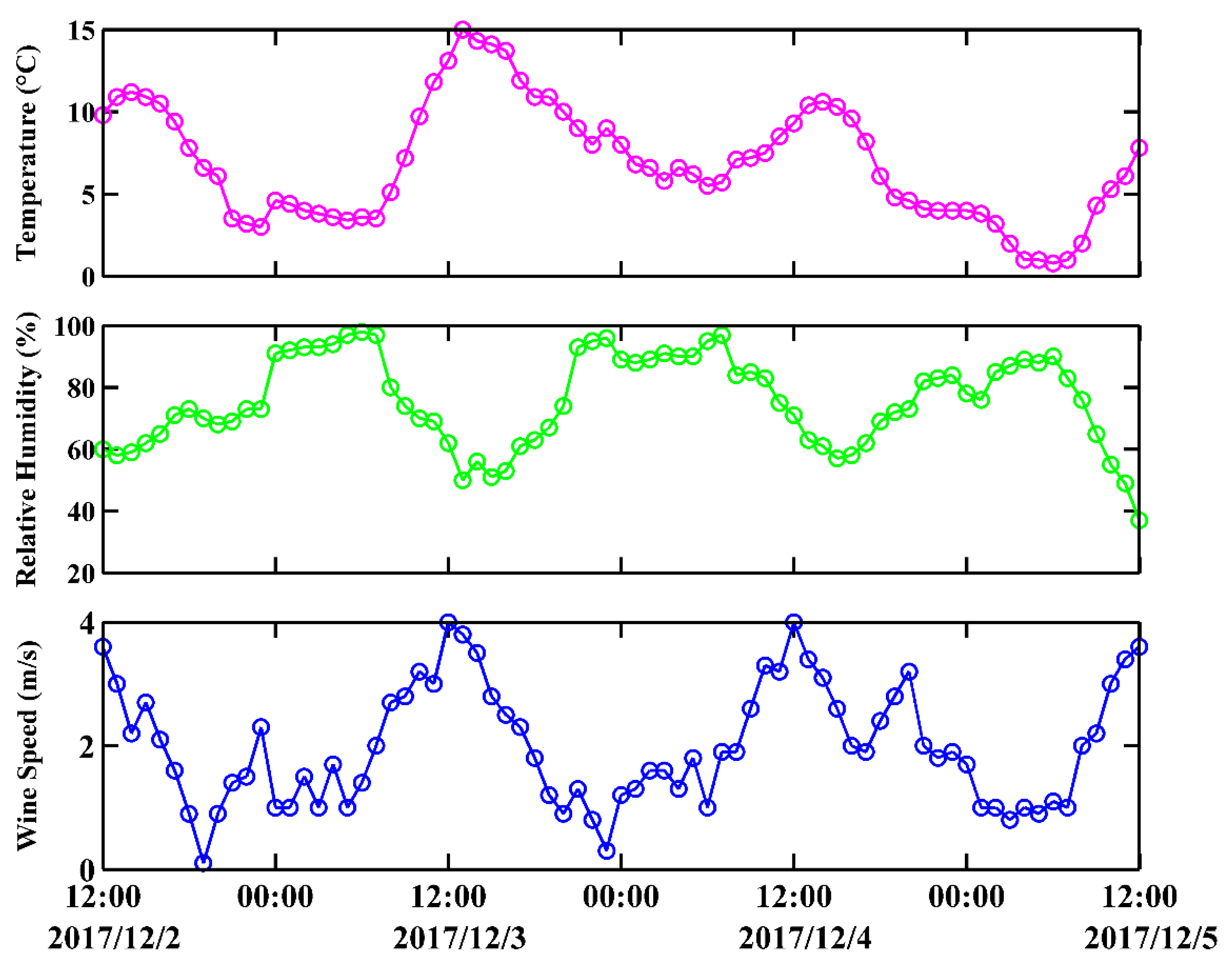
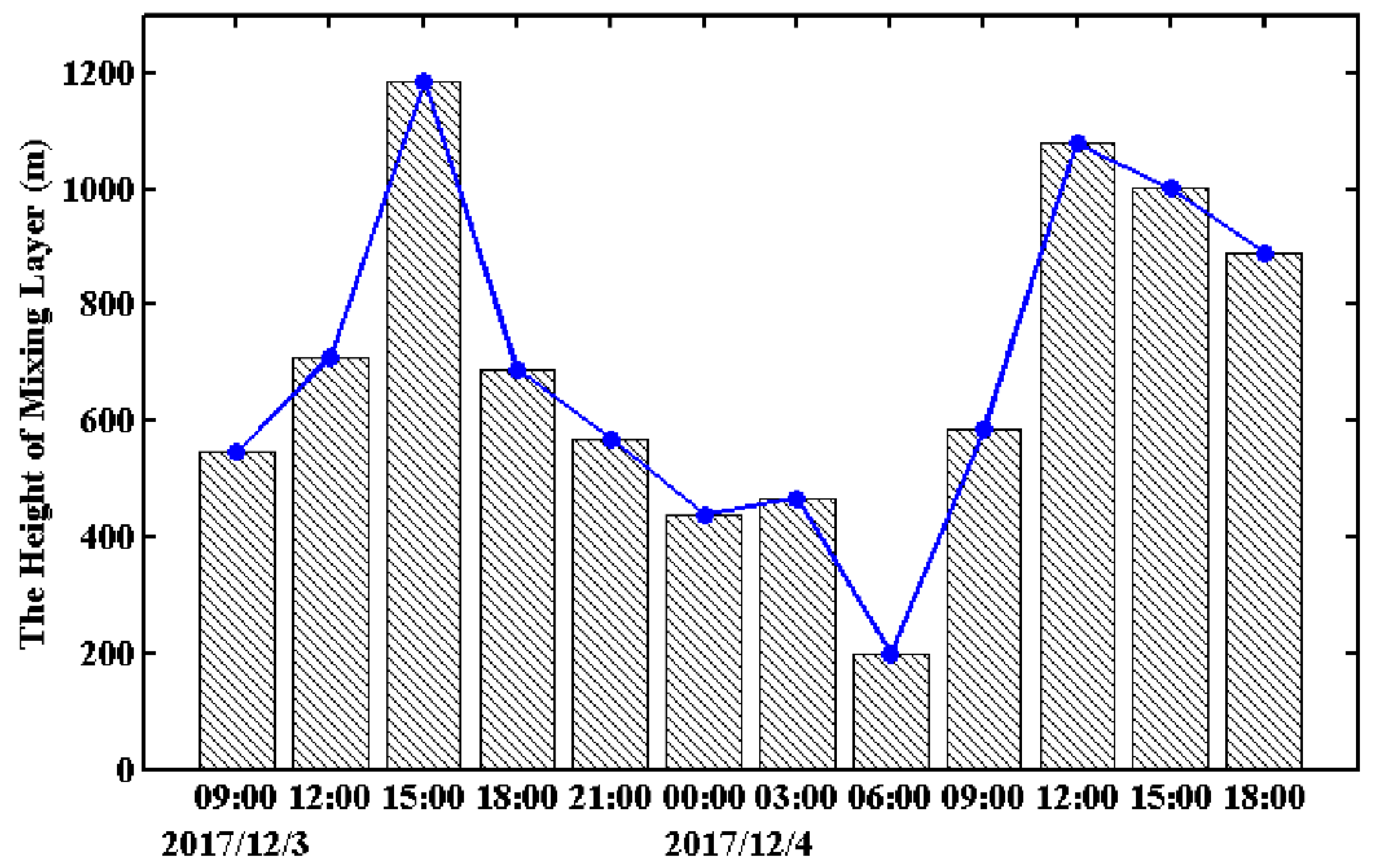
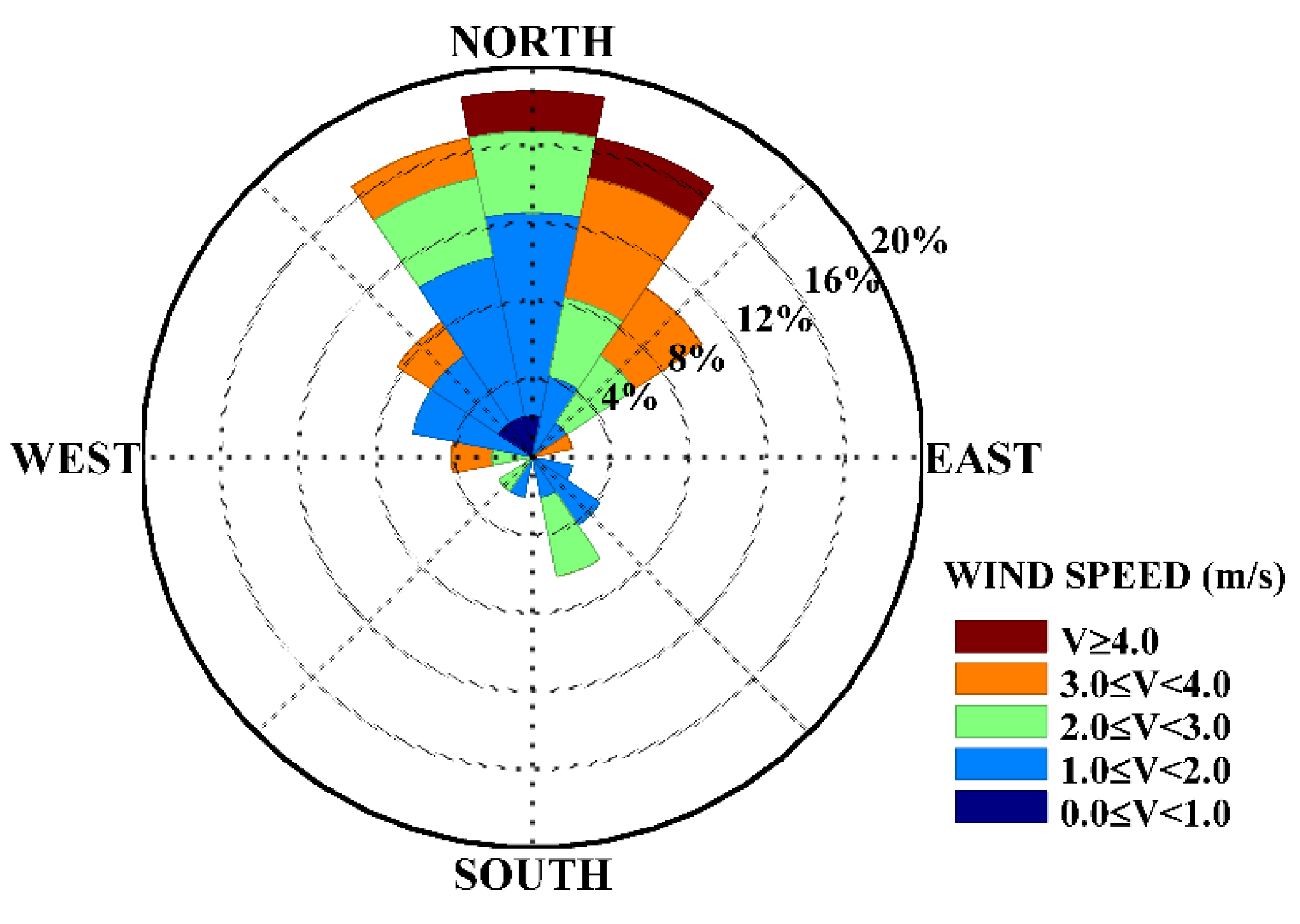
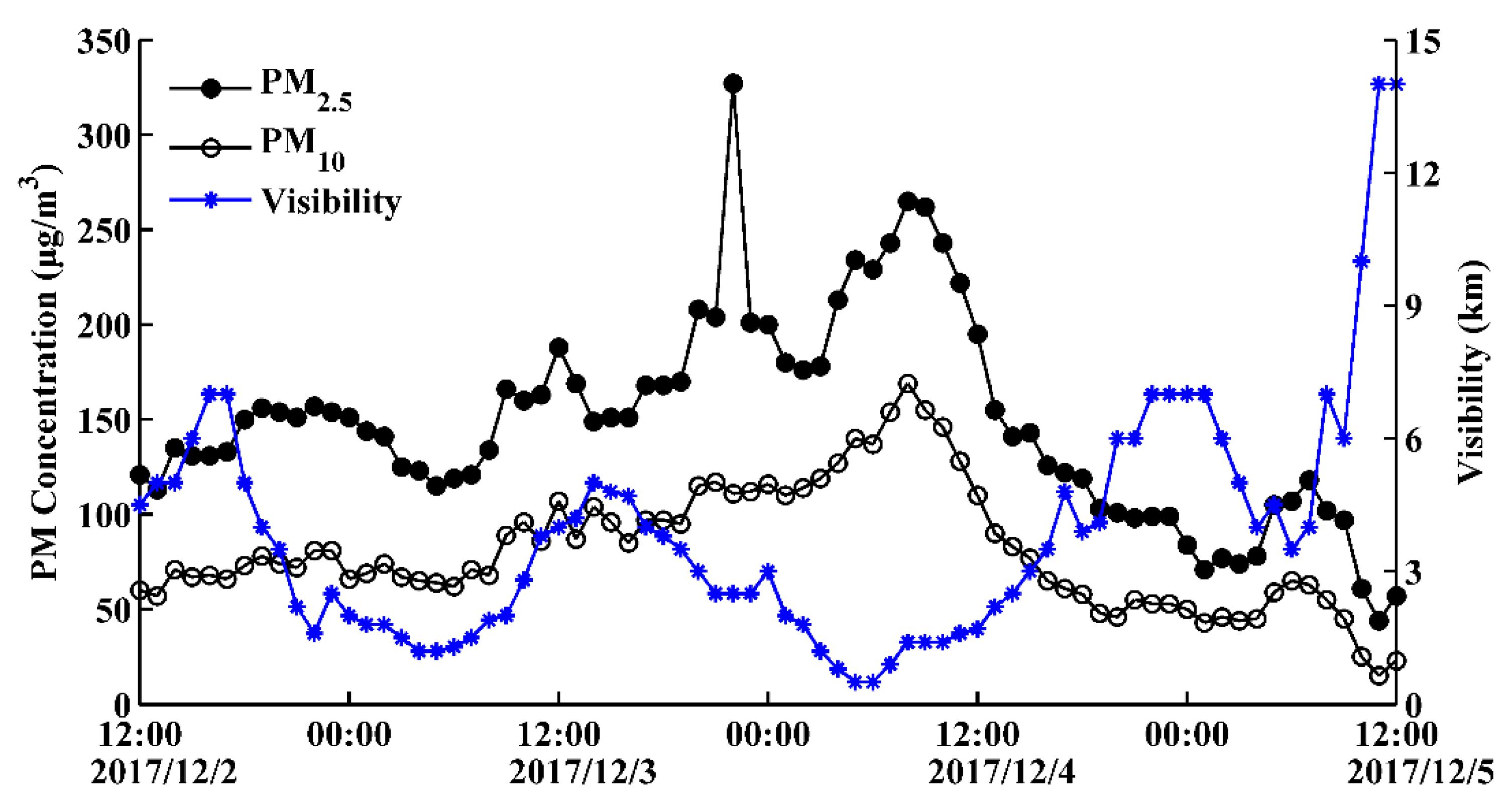
4.1. Pollution Episode Summary and Meteorological Factors

Figure 4 shows the temporal variation in the hourly surface PM (PM_2.5 and PM₁₀) mass concentration and visibility during the pollution episode. The mass concentration of PM_2.5 was in good accordance with that of PM₁₀. The PM mass concentration exhibited stable low levels from 12:00 LST on 2 December to 08:00 LST on 3 December and gradually increased with slight fluctuations after 09:00 LST. At 22:00 on 3 December, the PM₁₀ concentration reached a peak of 327 μg/m³. In addition, the mass concentrations of both PM_2.5 and PM₁₀ increased largely during 03:00–08:00 LST on 4 December and reached peaks of 169 and 265 μg/m³, respectively, at 08:00 LST, indicating the continuous accumulation of pollutants and serious pollution. Thereafter, the PM_2.5 and PM₁₀ mass concentrations decreased gradually, falling to 50 and 84 μg/m³, respectively, at 00:00 LST on 5 December. These values subsequently maintained low levels, reflecting the dissipation process of the pollutants. A relatively opposite variation in the visibility was observed compared with that of the PM mass concentration. With the gradual increase in the PM mass concentration after 14:00 LST on 3 December, the visibility fell from 6.5 km to 1–2 km. When the PM mass concentration decreased during the nighttime on 4 December, the visibility returned to 4 km and exceeded 10 km after 10:00 LST on 5 December. Furthermore, PM_2.5 was regarded as the primary pollutant during this process, and the daily PM_2.5 mass concentration on 3 and 4 December was 89 and 101 μg/m³, respectively, which exceeded the Grade II standard concentration (75 μg/m³ per 24 h). In addition, to demonstrate the spatial‒temporal variation in the surface PM_2.5 mass concentration, Figure 5 shows the PM_2.5 distribution at three-hour intervals in Jiangsu Province during the pollution episode based on the PM_2.5 measurements from China National Environmental Monitoring Center stations. A higher PM_2.5 mass concentration was observed in the northwestern region, which exceeded 250 μg/m³ at some sites. With the occurrence of high values moving southward, Nanjing and its surrounding areas suffered from varying levels of pollution. In addition, the PM_2.5 mass concentration decreased significantly from north to south, and the concentration over Nanjing dropped below 75 μg/m³ at 18:00 LST on 4 December, providing an initial indication for the transport path of the pollutants.

To demonstrate the effects of the surface meteorological elements on the accumulation and dissipation of PM_2.5, the hourly evolutions of the variables (temperature, relative humidity and wind speed) provided by automatic weather stations are depicted in Figure 6. At 09:00 LST on 3 December, the PM_2.5 mass concentration increased gradually and exceeded 75 μg/m³. The visibility peak at noon was lower than that at noon on the previous day. After 14:00 LST on 3 December, with an increase in the relative humidity and reductions in the wind speed and temperature, the dissipation of PM_2.5 was impeded, and the visibility decreased. After nightfall on 3 December, strong radiative cooling near the ground resulted in the fast condensation of water vapor and a substantial increase in the relative humidity. With a high relative humidity (>90%), low temperature (5–6 °C) and low wind speed (<2 m/s), the PM_2.5 mass concentration continued to increase significantly, reaching a peak at 08:00 LST on 4 December. The highest temperature of 10.6 °C was observed at 14:00 LST on 4 December, indicating an apparent temperature increase after noon due to solar radiation. Simultaneously, the relative humidity was reduced to less than 60%, and the wind speed increased to 2–4 m/s. Under this circumstance, the pollution became gradually relieved; the PM_2.5 mass concentration fell to less than 75 μg/m³ after 16:00 LST. In addition, as the invasion of cold air enhanced the dispersion potential of PM_2.5, the concentration remained at low levels (<60 μg/m³), and the visibility became better after nightfall on 4 December. Overall, the surface meteorological condition exerted a significant influence on the pollutant concentration in the atmosphere. Specifically, the high relative humidity, low wind speed, and low temperature were not conducive to pollutant dissipation.

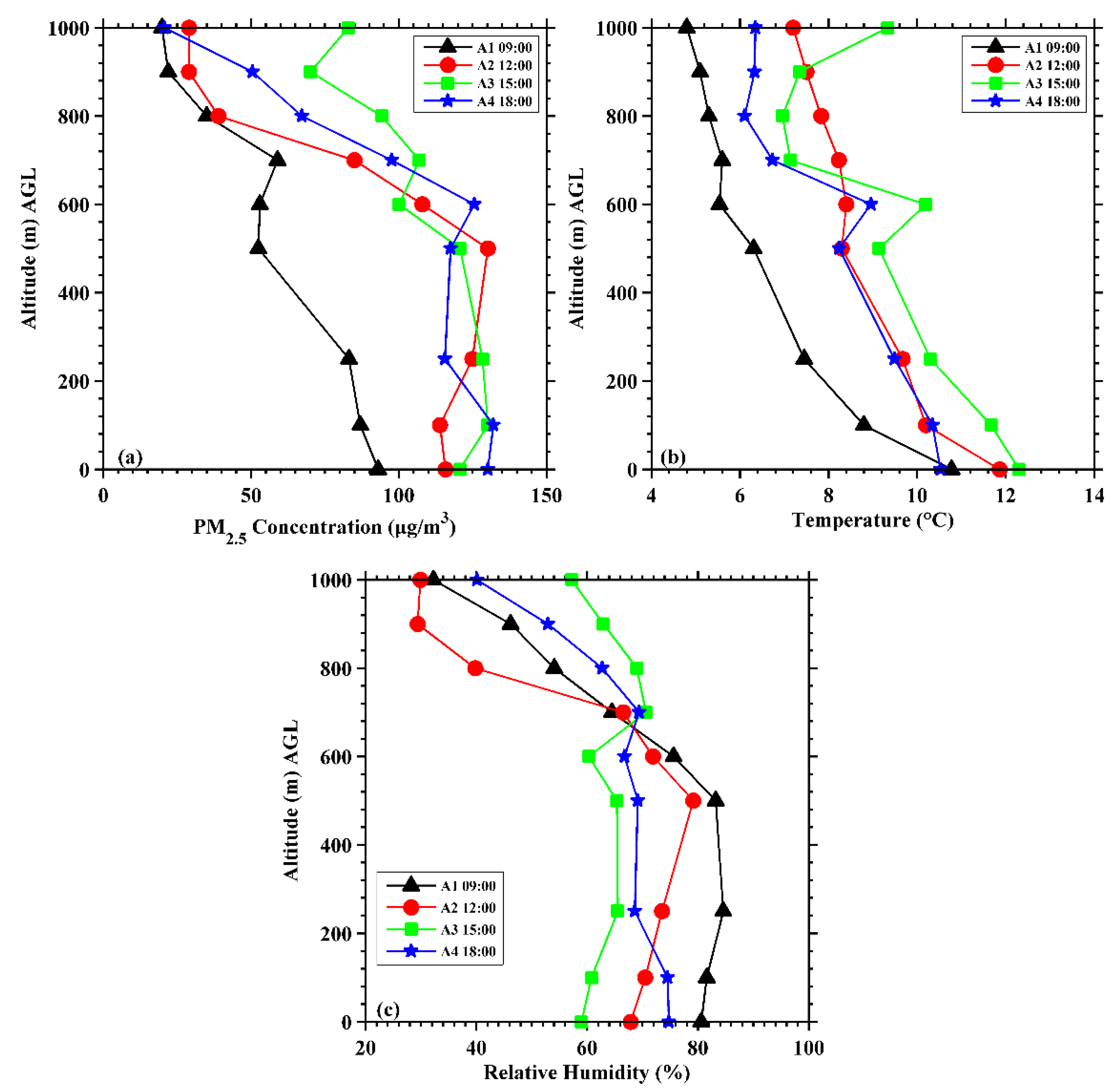
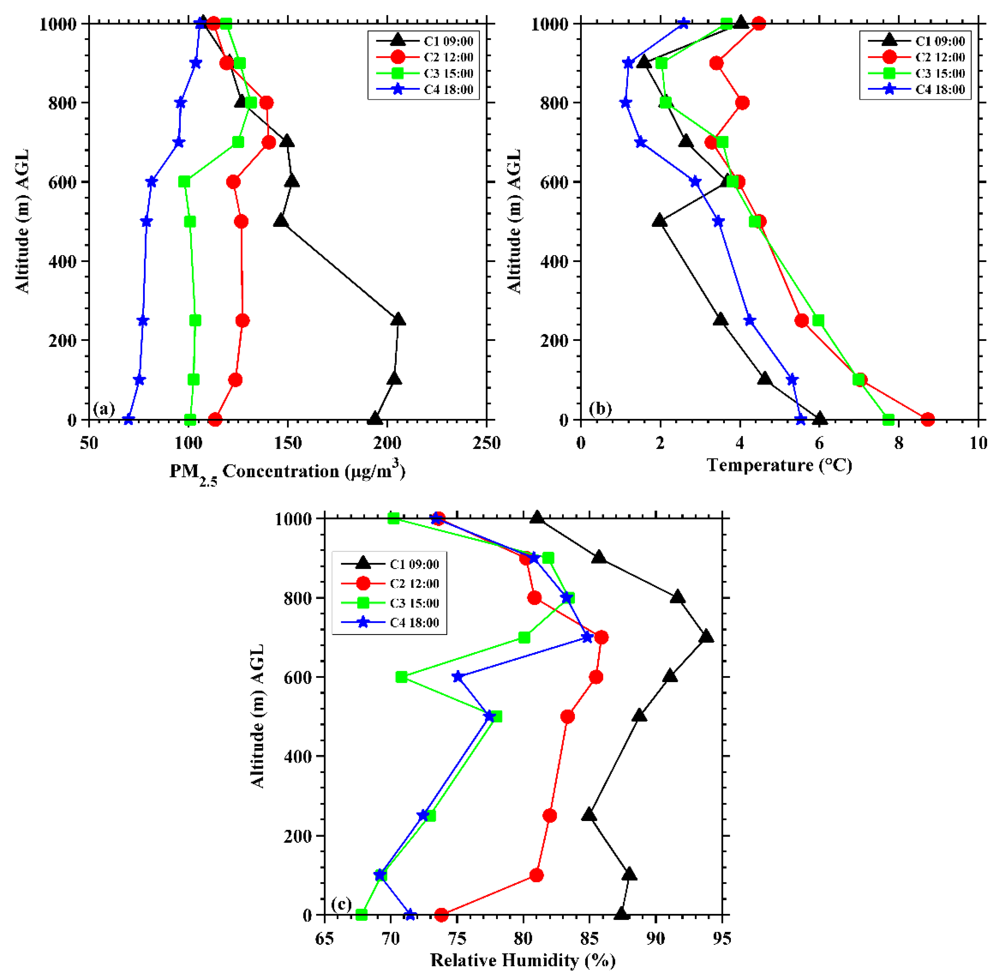
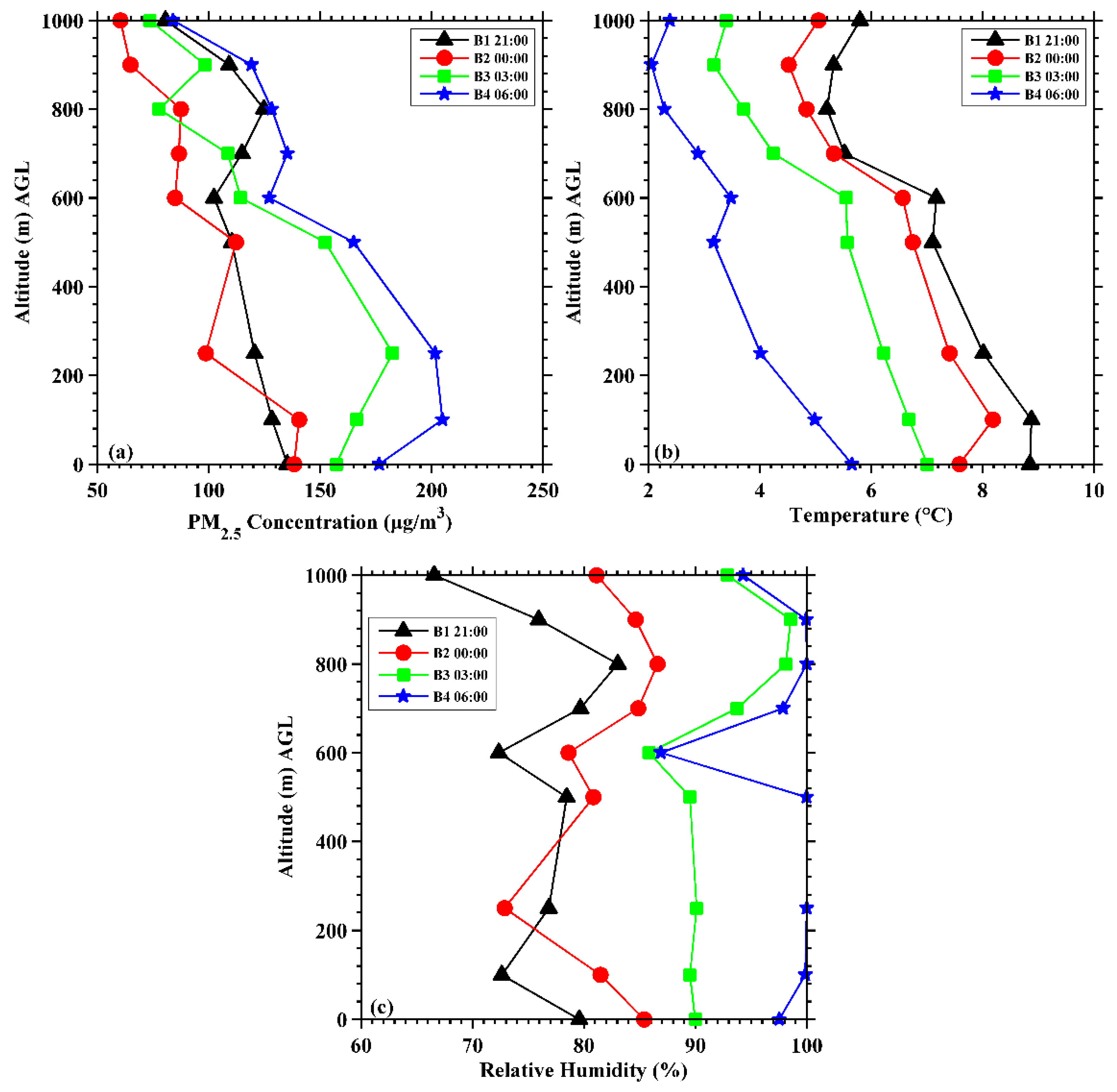
4.2. Flight Measurement Features

The vertical profiles of the PM_2.5 mass concentration, temperature and relative humidity were acquired through UAV experiments. On average, the PM_2.5 mass concentration at the surface (0 m AGL) sampled by the UAV was slightly higher than that of the surface measurement at the Xianlin University Town monitoring site. Through analysis, it may be affected by not only differences in the detection equipment and measurement principle but also the ambient conditions. In addition, the variations in the two measurements had the same trend.

The first four flights were carried out during the daytime from 09:00 to 18:00 LST on 3 December. The profiles of the variables are presented in Figure 7. Each flight showed a high PM_2.5 mass concentration on the ground ranging from 93 to 131 μg/m³ (Figure 7a). For flight A1, the PM_2.5 mass concentration decreased significantly as the altitude increased with a slight inversion between 500 and 700 m AGL. For flight A2, a high PM_2.5 mass concentration was observed with little notable change between the surface and 600 m AGL, and the highest concentration reached 130 μg/m³ at 500 m AGL. Combined with the vertical profiles of the temperature (Figure 7b), it could be inferred that the temperature inversion layer formed between 500 and 600 m AGL. In most cases, the temperature inversion layers formed during a pollution event could restrain convection and favor the accumulation of particulate matter, thereby inhibiting the vertical diffusion of PM_2.5 [34]. Flights A3 and A4 also exhibited relative homogeneity in the PM_2.5 mass concentration as the altitude increased below 600 m AGL, and the intensity of the temperature inversion layer remained stable and strong. For flight A3, an increase in the PM_2.5 mass concentration at 1000 m AGL was found. Through analysis, it may not be caused directly by the temperature inversion layer formed from 900 to 1000 m AGL, because the concentration decreased distinctly as altitude increased between 700 and 900 m AGL. This phenomenon may be related to the horizontal transport at high altitudes. For flight A4, the concentration rapidly decreased as the altitude increased above 600 m AGL, indicative of the remission of pollution at high altitudes. The altitude dependency of the measured relative humidity during flights A1, A2 and A4 presented similar variations, which decayed in a fluctuating trend with the altitude, and the values were approximately <80% at each altitude (Figure 7c). For flight A3, the relative humidity became uniform and was approximately 65%, which extended throughout the sampling altitudes. Overall, the temperature inversion layer contributed more to the increasing PM_2.5 mass concentration during the daytime because of its impact on inhibiting the vertical diffusion of particles. In addition, the concentration was relatively low between 800 and 1000 m AGL and high between the surface and 700 m AGL, which may be related to local pollution.

Fights B1, B2, B3 and B4 occurred during the evening of 3 December and the early morning of 4 December. The profiles of the variables are illustrated in Figure 8. The PM_2.5 mass concentration at the surface was significantly higher than that in the daytime, ranging from 135 to 176 μg/m³ (Figure 8a). In addition, the temperature decreased successively over time at each altitude. For fights B1 and B2, the vertical variation in the PM_2.5 mass concentration and temperature (Figure 8b) exhibited good consistency respectively. Furthermore, high values of the relative humidity during the two flights were observed at 800 m AGL, as shown in Figure 8c. For flights B3 and B4, the vertical profiles of the PM_2.5 mass concentrations, temperature and relative humidity showed consistent trends, respectively. Figure 8c shows that the relative humidity during flights B3 and B4 reached approximately 90% and 95%, respectively, at each altitude except 600 m AGL. In addition, the PM_2.5 mass concentration exceeded 110 μg/m³, and the highest value reached 204 μg/m³ between the surface and 700 m AGL for both flights. In general, the relative humidity was also a significant factor for the accumulation of PM_2.5. Research has shown that a higher relative humidity is conducive to an increase in the PM_2.5 mass concentration because it can not only change the optical properties of particulate matter and help trigger hygroscopic growth, but also promote the transformation of pollutants to PM_2.5 through physical and chemical processes [35]. Overall, the higher relative humidity helped facilitate the accumulation of PM_2.5, especially at midnight and during the early morning, which indirectly indicated that the level of pollution and relative humidity were positively correlated. In addition, during this period the increasing amount of water vapor could accelerate the formation of particulate matter, and the lower temperature was not conducive to the convection in the atmosphere, which was detrimental to the dissipation of pollutants. These factors contributed mutually to the increase in PM_2.5. Furthermore, the PM_2.5 mass concentration between 700 and 1000 m AGL during the four flights was higher than that during the daytime, which was likely related to the continuous transport of pollutants at high altitudes. Simultaneously, the pollutants at low altitudes accumulated when the horizontal transport of those at high altitudes sank down.

The last four flights (C1, C2, C3, and C4) occurred during the daytime on 4 December. The altitude dependence of each variable is depicted in Figure 9. The PM_2.5 mass concentration decreased successively over time at each altitude between the surface and 700 m AGL (Figure 9a). In particular, the concentration at the surface was reduced from 193 to 69 μg/m³ as time progressed, indicating gradual pollutant dissipation. However, the concentration of the four flights at 900 and 1000 m AGL respectively exhibited small variations and exceeded 100 μg/m³. Figure 9b shows that the formed temperature inversion layers still existed, and the intensity of the inversion layer from 500 to 600 m AGL gradually decreased, while the inversion layer from 900 to 1000 m AGL was still strong. Figure 9c reveals that the relative humidity during the four flights generally increased with the altitude between the surface and 700 m AGL and decreased above 700 m AGL. For flight C1, the relative humidity remained higher throughout the sampling flight profile, as the increase in the temperature from radiative heating was not distinct. Overall, although the pollution was generally alleviated over time as a whole, a high PM_2.5 mass concentration was observed at 900–1000 m AGL. Through analysis, the formed temperature inversion layer between 900 and 1000 m AGL may not be the major reason, as the PM_2.5 concentration was relatively low at lower altitudes. This phenomenon may mainly come from the persistent regional transmission of pollutants at higher altitudes.

Figure 10 shows the temporal variation in the thickness of the atmospheric mixed layer according to Equation (3) at three-hour intervals based on the sampled variables during the flight sampling. The thickness depicted was below 1200 m during this event with the diurnal variation characteristics of high values in the daytime and low values at night. The thickness of the mixed layer showed an evident declining trend after 15:00 LST on 3 December, and it fell to 200 m at 06:00 LST on 4 December corresponding to the period of aggravated pollution. This indicates that the lower mixed layer thickness was closely correlated with the pollution levels, as it could inhibit convective transport in the vertical direction and simultaneously weaken the vertical diffusion potential of atmospheric pollutants with small horizontal wind speeds (Figure 6), leading to the retention and accumulation of PM_2.5. Apparently, after 12:00 LST on 4 December, the thickness of the mixed layer was higher, which could have strengthened the capacity of atmospheric diffusion in this region.

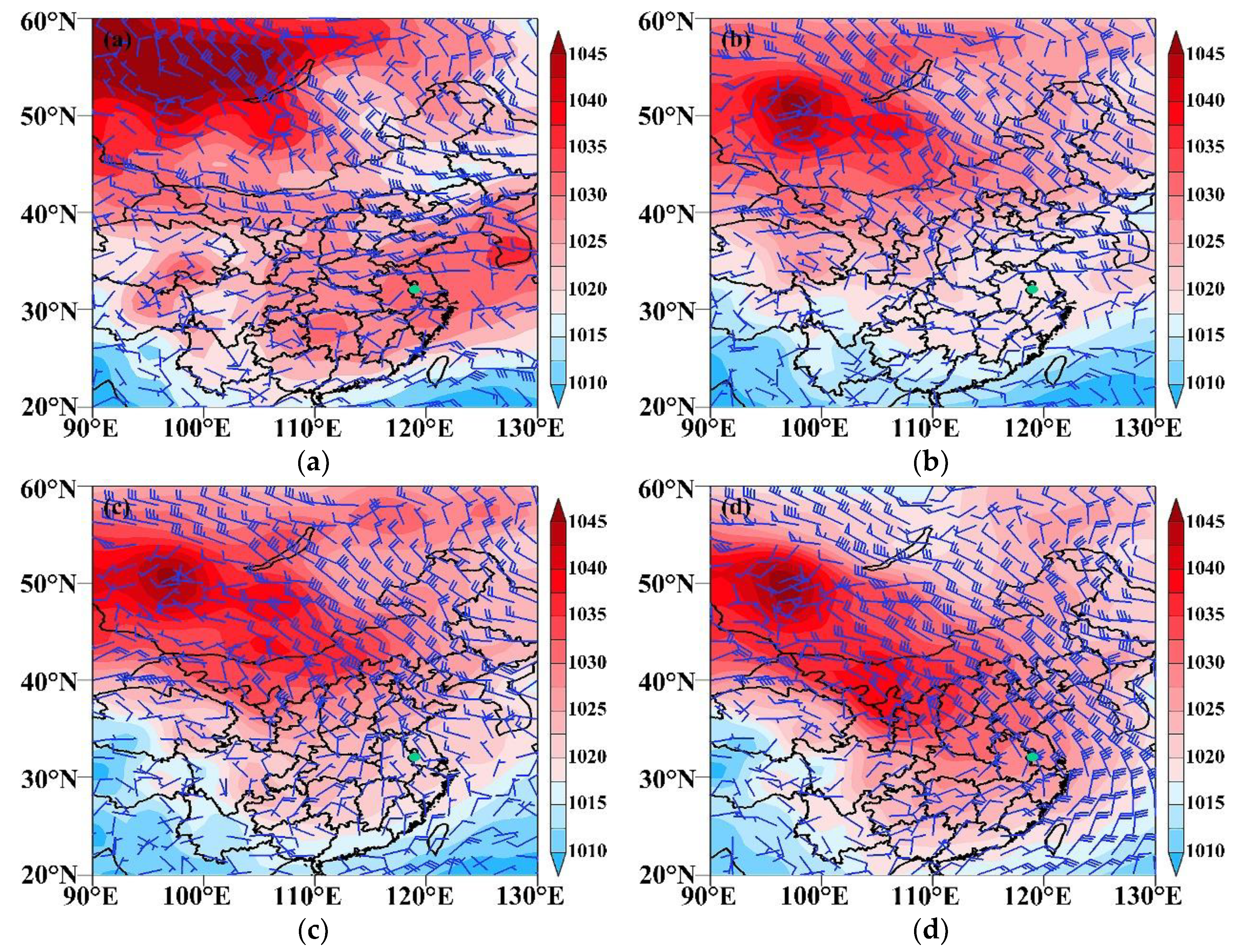
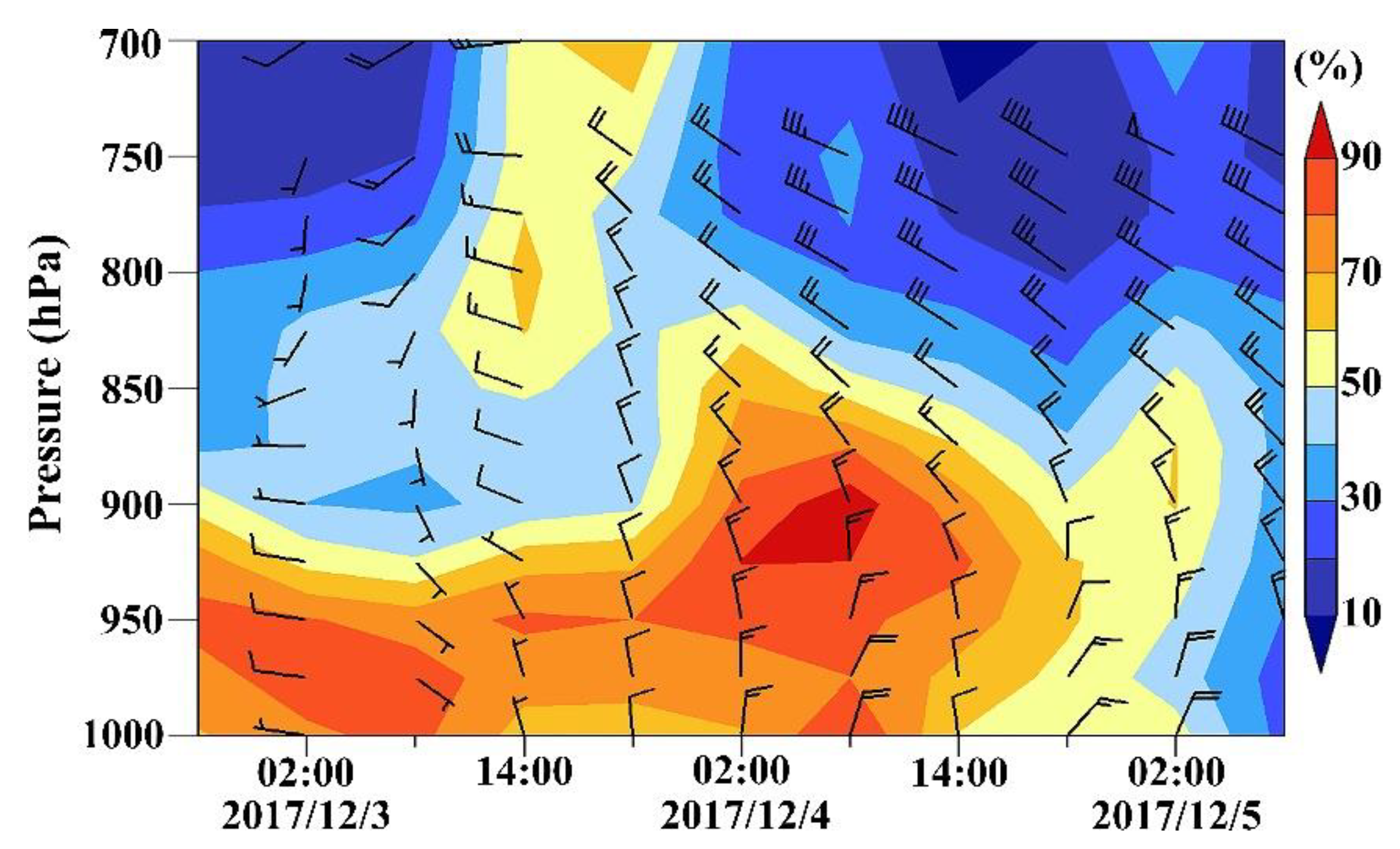
4.3. Synoptic Situation

An analysis of the synoptic situation could provide an indication for the variation and characteristics of the pollution episode as a whole. The observed distributions of the sea level pressure field and the horizontal wind field at 850 hPa based on the NCEP FNL 1° × 1° grid data during this event are correspondingly depicted in Figure 11.

At 500 hPa on 1 December, two troughs (one located to the east of the Ural Mountains and the other over the southern part of Lake Baikal) and one ridge (located between the two troughs) were depicted at the mid‒high latitudes of Eurasia, and a westward flat flow occupied the dominant position in the absence of distinct troughs and ridges over the central and eastern parts of China, which was detrimental to the cold air outbreak. At 08:00 LST on 2 December (Figure 11a), the Siberian high pressure system was located to the north of China, coincident with the formation of strong, cold air masses. The Beijing-Tianjin-Hebei (BTH) region (113–120° E, 36–43° N) was under the control of the homogeneous pressure field distribution, which maintained a stable circulation. The southwesterly winds passing over the southern part of the BTH region at 850 hPa led to enhanced pollutant transport. Coupled with local emissions and the lower boundary layer, this condition resulted in a sharp increase in the PM_2.5 mass concentration and a rapid expansion of the extent of pollution in the BTH region and its surrounding areas according to the monitoring sites. At 08:00 LST on 3 December (Figure 11b), the cold front and the stronger northwesterly wind passed over the BTH region, which improved the air quality in the region. Simultaneously, the haze ahead of the cold air masses also moved toward the south and gradually influenced Jiangsu Province, where the synoptic situation was stable at this point. At 20:00 on 3 December (Figure 11c), the northwesterly wind was observed strong from the BTH region to the northern parts of Jiangsu Province at 850 hPa, which transported pollutants and would lead to the distinct accumulation of PM_2.5 mass concentration in Nanjing. Nanjing and its surrounding areas were still under a condition of weak and homogeneous pressure, and the small pressure gradient resulted in small wind speeds, which were indicative of the poor diffusion of PM_2.5. At 14:00 on 4 December, as the strong cold air masses continued to move southward, the wind speeds in Nanjing at 850 hPa increased rapidly. Up to 20:00 on 4 December (Figure 11d), the surface PM_2.5 mass concentration decreased sharply with the dispersion and transference of the pollutants. Therefore, appropriate synoptic circulation (i.e., a homogenous pressure field and low wind speed) could have led to the formation of regional pollution and the accumulation of pollutants in the early stage. The transport of pollutants from the BTH region and its surrounding areas with strong northwesterly winds may have contributed more to the PM_2.5 increase in Nanjing during the period of pollution aggravation.

Higher-precision ECMWF grid reanalysis data were referenced for this analysis. The vertical distributions of the horizontal wind field and relative humidity throughout the grid (32.125° N, 119° E) are depicted from 02:00 LST on 3 December to 02:00 LST on 5 December (Figure 12). The low-level wind speed was small and the wind direction was unstable during 02:00–14:00 LST on 3 December due to the homogenous pressure field, which obstructed the diffusion of pollution emissions. After 20:00 LST on 3 December, the primary northerly and northwesterly winds occupied the levels between 1000 and 700 hPa, and they became strengthened above 850 hPa, indicative of the southward transport of strong, cold air with pollutants. In addition, the relative humidity increased and exceeded 90% at approximately 900 hPa coincident with the temperature inversion during the night, leading to a rapid increase in the PM_2.5 mass concentration. After 14:00 LST on 4 December, the relative humidity under 850 hPa was obviously reduced. Meanwhile, the strong northwesterly wind above 850 hPa persisted and continuously transported pollutants, while the northeasterly wind appeared near the surface, which would dissipate pollutants. The statistics for the surface wind and direction during 3–4 December, as depicted in Figure 13, indicated that the dominant wind directions were north, north-northwest and north-northeast, accounting for 18.75%, 16.66%, and 16.66%, respectively. In addition, the wind speed mainly ranged from 1 to 3 m/s, and the average was 2.11 m/s during this event.

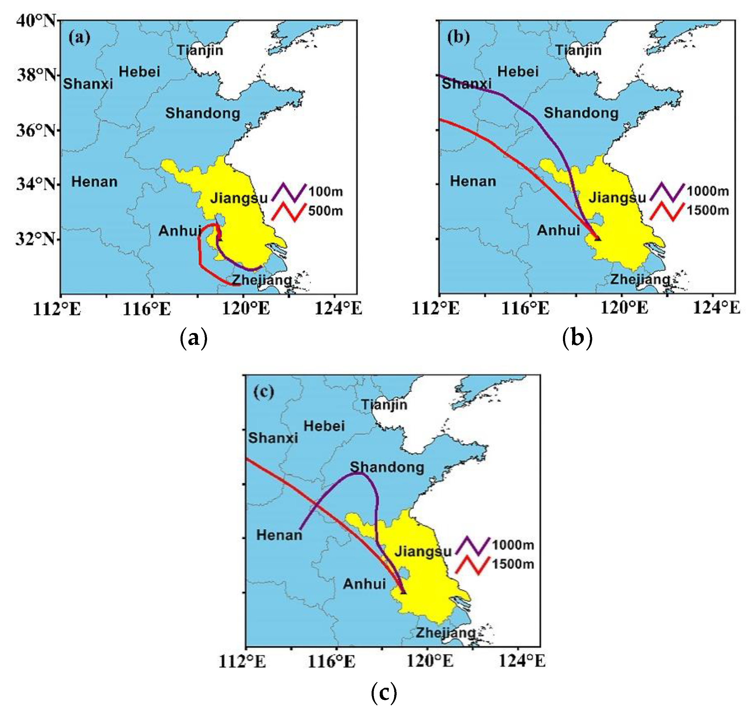
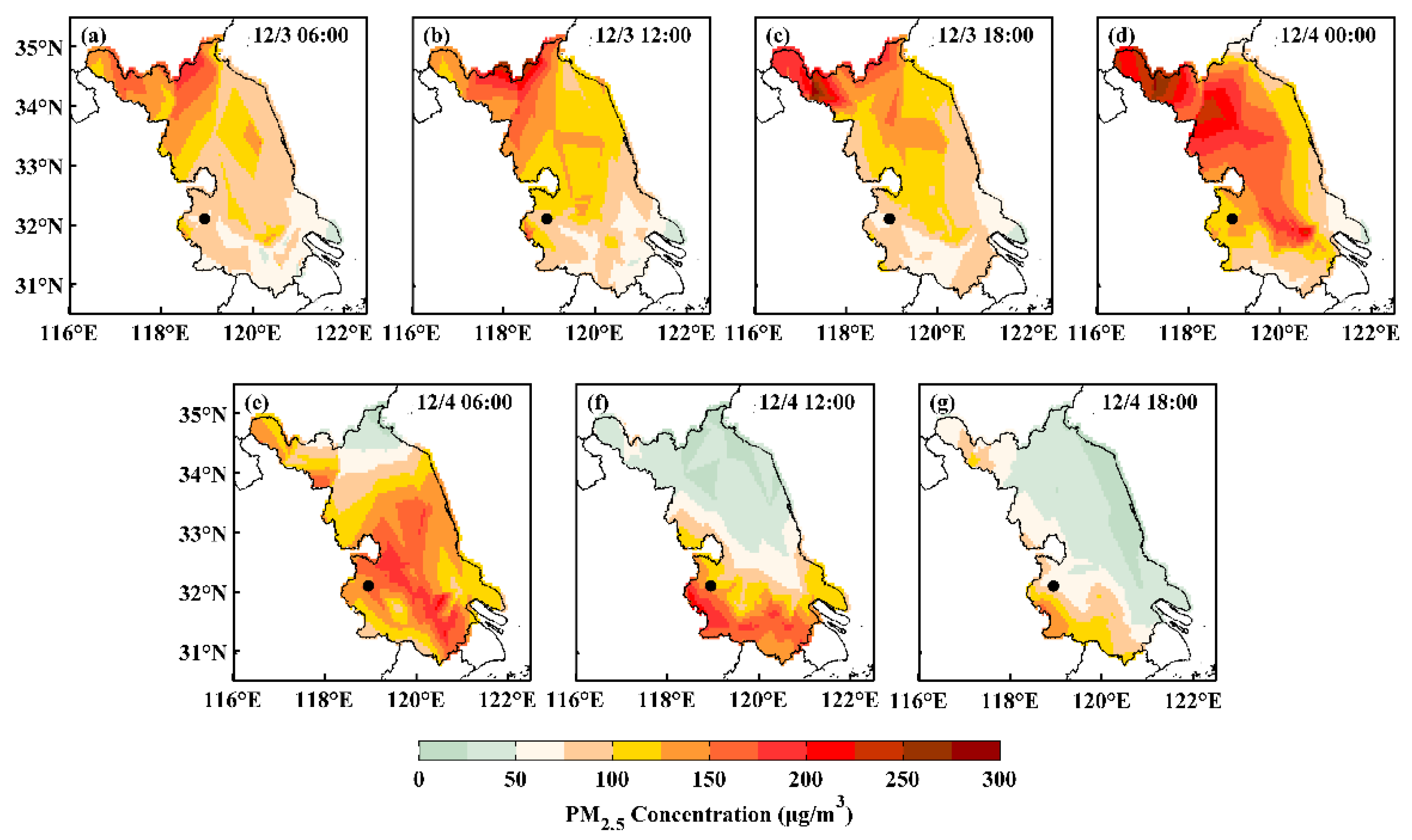
4.4. Major Contributions and Transport Pathways in the Pollution Episode

An analysis of the distribution of the PM_2.5 mass concentration and the synoptic situation described above suggests that the elevated local pollutants might be attributed to pollutants from the north, such as the BTH region and its surrounding areas. Furthermore, the backward trajectory model adopted has significant implications for determining the potential source areas that contributed to the pollution episode and the transport pathways of the pollutants.

Figure 14 depicts the calculated 48-h backward trajectories during the pollution episode. The experiment site mentioned above served as the starting point for simulating the trajectories. For the same simulation time, the longer the trajectory is, the faster the transport process [36]. Figure 14a presents the calculation results at 18:00 LST on 3 December. Because the high PM_2.5 mass concentration was mainly between the surface and 700 m at that time, the lower layers (100 m and 500 m) were chosen as the initial altitudes for the calculation. The trajectories were from the south, passing over the areas to the south of Nanjing, and the lengths were relatively shorter, suggesting that pollution emissions such as combustion products (e.g., coal or straw burning in the winter) from the local or surrounding areas could contribute more to increases in the PM_2.5 mass concentration in combination with the stable synoptic situation [37] (Figure 11c). Due to the propagation of cold air and the development of winds at higher altitudes, the higher layers (1000 m and 1500 m) were regarded as the initial altitudes to explore the trajectories at 08:00 and 18:00 LST on 4 December. The trajectories at 08:00 LST were from the northwest, and they passed over central-eastern China (Shanxi, Hebei and Shandong Province at 1000 m; Shanxi, Henan, and Anhui Province at 1500 m) (Figure 14b). The trajectories as well as the elevated PM_2.5 indicated that long-range or regional transport pathways provided more contributions. At 18:00 LST (Figure 14c), the trajectory at 1500 m was consistent with that at 08:00 LST. The trajectory at 1000 m moved from Henan Province toward Nanjing in an anticyclonic fashion. With the relatively high PM_2.5 mass concentration observed by the UAV at 900–1000 m, the long-range transport of pollutants was more likely to persist.

Compared with the pollution emissions from the local or surrounding areas, long-range transport from the north, such as the southern BTH region and its surrounding areas, which were characterized by high emissions of particulate matters caused mainly by central heating during the wintertime, occupied the dominant factor in the increasing mass concentration of PM_2.5. The cities around the trajectories, including Taiyuan (Shanxi Province), Shijiazhuang (Hebei Province), Zhengzhou (Henan Province), Jinan (Shandong Province), and Bengbu (Anhui Province), during 1–5 December suffered from different levels of pollution (

Table 2. The air quality index in Taiyuan, Shijiazhuang, Zhengzhou, Jinan, and Bengbu.

Date	Taiyuan (Shanxi)		Shijiazhuang (Hebei)		Zhengzhou (Henan)		Jinan (Shandong)		Bengbu (Anhui)
	AQI	Air Quality Level	AQI	Air Quality Level	AQI	Air Quality Level	AQI	Air Quality Level	AQI	Air Quality Level
01 Dec	110	Lightly Polluted	152	Moderately Polluted	168	Moderately Polluted	112	Lightly Polluted	92	Good
02 Dec	172	Moderately Polluted	248	Heavily Polluted	216	Heavily Polluted	130	Lightly Polluted	109	Lightly Polluted
03 Dec	109	Lightly Polluted	254	Heavily Polluted	286	Heavily Polluted	166	Moderately Polluted	144	Lightly Polluted
04 Dec	58	Good	89	Good	190	Moderately Polluted	56	Good	155	Moderately Polluted
05 Dec	72	Good	68	Good	73	Good	75	Good	158	Moderately Polluted

). Among these cities, Taiyuan was moderately polluted on 2 December and was relieved subsequently. Shijiazhuang and Zhengzhou were heavily polluted on 2–3 December, where the circumstances were more serious, and the pollution was gradually reduced after that. The pollution became worse in Jinan on 3 December and in Bengbu after 3 December, indicative of the pollution zones moving south during that period.

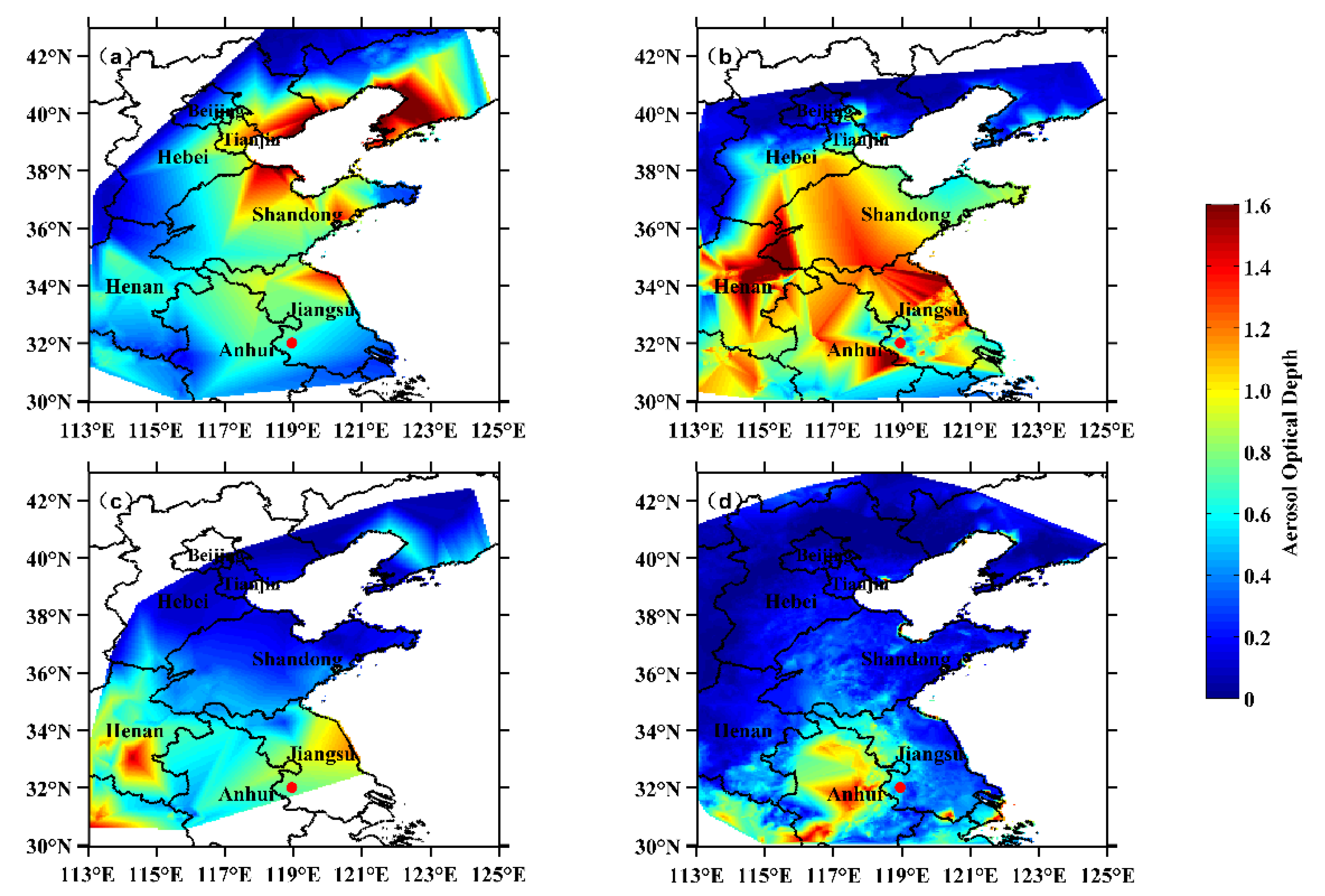
4.5. The Analysis of Satellite Remote Sensing Data

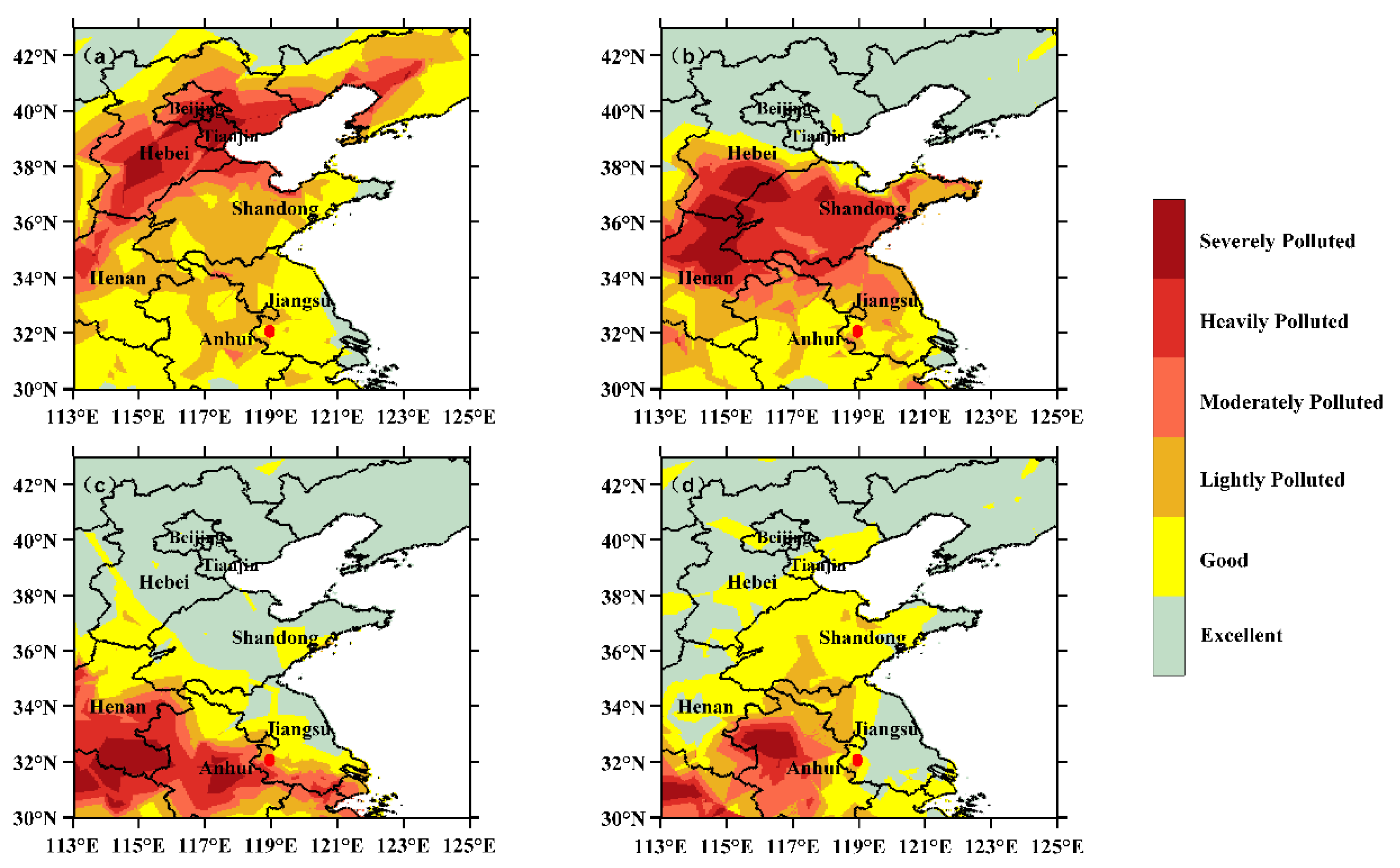
4.5.1. Analysis of the Distribution of the MODIS Aqua Satellite Retrieval AOD Product

The AOD is the integral of the aerosol extinction coefficient in the vertical direction, indicating the light attenuation resulting from columnar aerosols in the atmosphere. Higher AOD values illustrate greater attenuation and more severe pollution. Satellite remote sensing can provide the regional distribution of aerosol pollutants with a good spatial coverage. To demonstrate the features of aerosol pollutants during this episode, Figure 15 shows the AOD distribution in the eastern areas of China (113–115° E, 30–43° N) during 2–5 December. It is important to note that the Aqua satellite transited the above areas at approximately 14:00 LST, and the AOD is not displayed over some parts due to cloud cover and missing data, leading to an ineffective spatial interpolation. At approximately 14:00 LST on 2 December, the AOD in Nanjing and southern Jiangsu Province was low, while in parts of the BTH region and Shandong Province, it was high. At approximately 14:00 LST on 3 December, ranges of higher AOD (>1.0) were expanded mainly in Shandong, Henan and northern Jiangsu Province. Simultaneously, aerosol deposition began to appear gradually in Nanjing, and the AOD increased up to approximately 0.7. The AOD in Nanjing exceeded 0.9 at approximately 14:00 LST on 4 December, indicating the aggravation of pollution. Until 14:00 LST on 5 December, the AOD in most areas, including Nanjing, fell to less than 0.5, indicating the dissipation of pollutants. There was a close correlation between the monitored air quality and AOD. Based on the AQI data from the China National Environmental Monitoring Center stations, zones that were more seriously polluted (≥moderately polluted) moved toward the south with time, and the pollution was subsequently concentrated in Anhui Province, which is on the west of Jiangsu Province, on 5 December, as depicted in Figure 16. At 14:00 LST on 2, 3, 4, and 5 December, the air quality in Nanjing suggested good, lightly polluted, moderately polluted and good levels, respectively. Therefore, combined with the AOD and air quality with respect to the spatial distributions, a positive correlation between the accumulation of aerosol pollutants and the aggravation of pollution could provide an indication for the long-distance transport characteristics of pollutants, which is in good agreement with the northwest backward trajectory depicted in Figure 14b,c. Overall, the AOD and air pollution level were positively correlated, and they were obviously characterized by high-value (>1.0) AOD zones and zones of more serious pollution (≥moderate pollution) moving toward the south. The AOD increased (>0.9) with the aggravation of pollution while the AOD decreased (<0.5) with the reduction of pollution in Nanjing during the episode.

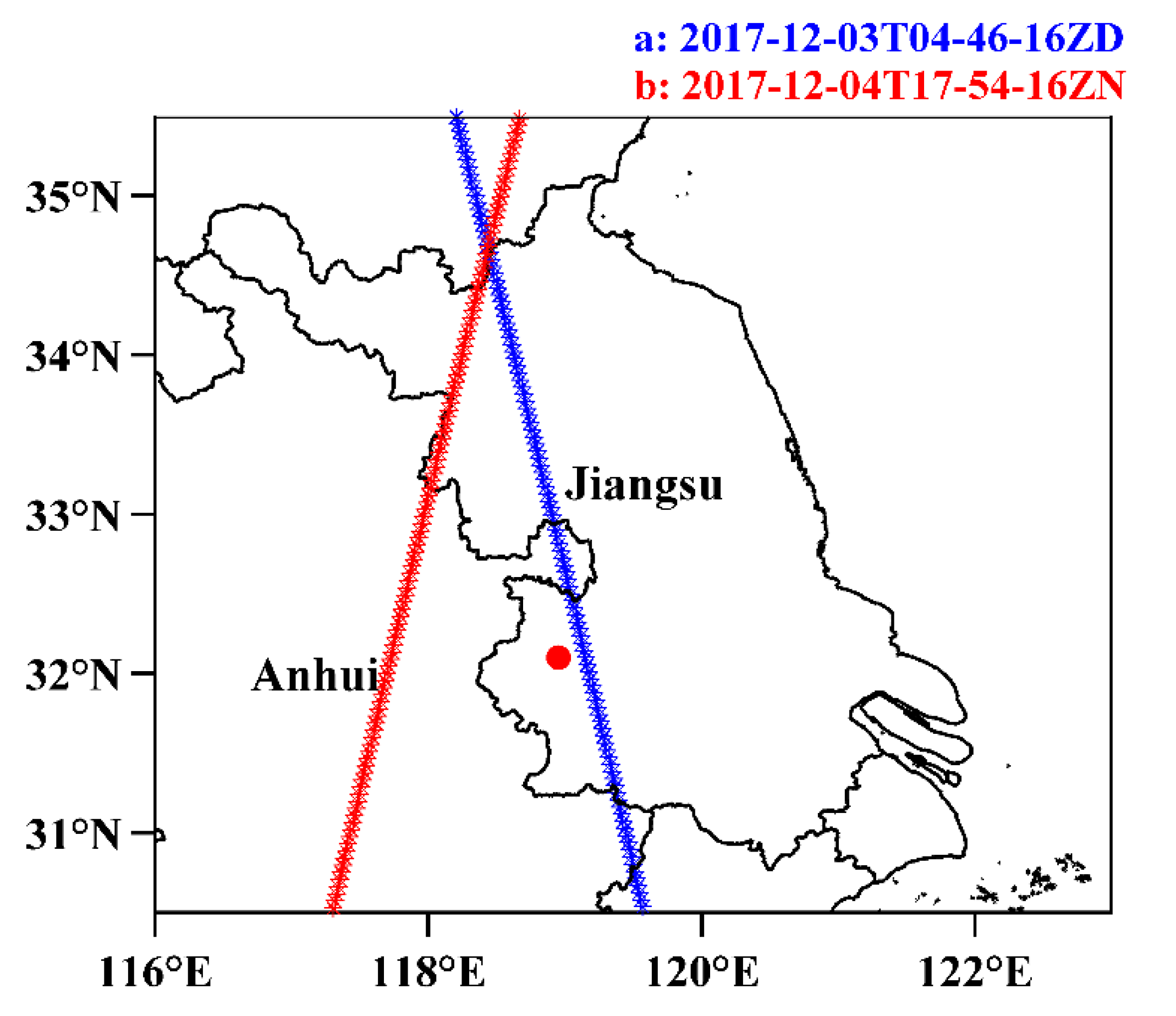
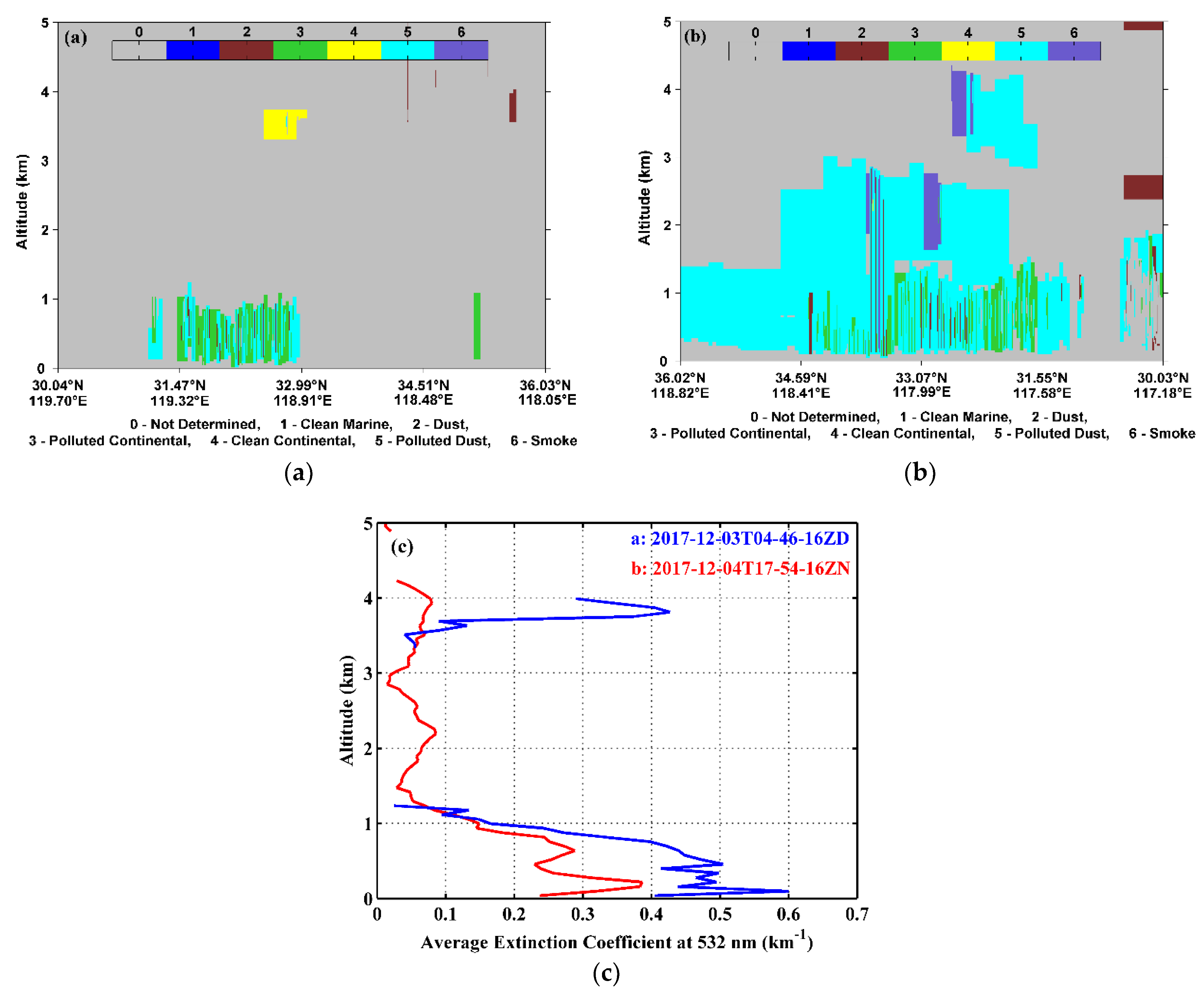
4.5.2. Analysis of the Vertical Distribution Characteristics of Aerosols

It is an issue worth exploring to analyze the characteristics of the vertical distribution of aerosols during this pollution episode. At approximately 13:00 LST on 3 December and 02:00 on 5 December 2017, the CALIPSO satellite transited the regions in and close to Jiangsu Province (approximately 117–120 °E, 30–36 °N); the orbit tracks were 2017-12-03T04-46-16ZD and 2017-12-04T17-54-16ZN, respectively, as depicted in Figure 17. The former corresponded to the gradual accumulation of pollutants, and pollution emissions from local or surrounding areas contributed more to Nanjing at this time. The latter corresponded to the dissipation of pollutants in Nanjing, and the pollution was concentrated in Anhui Province at this time with the transport of pollutants, which could also provide an indication for the vertical distribution characteristics of aerosols during the event.

Figure 18 shows the vertical distribution of aerosol types and the vertical profiles of the average extinction coefficient at 532 nm over the region depicted as lines in Figure 17. At approximately 13:00 LST on 3 December, polluted continental aerosols and polluted dust aerosols primarily existed from the surface to 1 km in the region (118.91–119.32° E, 31.47–32.99° N) near Nanjing (Figure 18a). In addition, higher values of the average extinction coefficient were concentrated in the layer below 0.5 km ranging from 0.4 to 0.6 km⁻¹, and they decreased with increasing altitude below 1.2 km (Figure 18c), indicating that the pollutants were mainly concentrated at lower altitudes and that they were affected by emissions from the local or surrounding areas, which is consistent with the above discussion. In addition, the average extinction coefficient in the layer at 3.3–4 km was mostly related to the observed clean continental aerosols. At approximately 02:00 LST on 5 December, the polluted dust aerosols accounted for the major part and existed from the surface to 3 km, and they even exceeded 4 km in the region (117.58–118.41° E, 31.55–34.59° N), which represents northwestern Jiangsu and the central part of Anhui Province (Figure 18b). It is worth mentioning that polluted dust aerosols mainly consisted of aerosols formed by man-made emissions and dust particles that were most likely originated from the sand source region to the west of the BTH region, and they were likely transported toward the south with strong northwesterly winds. Simultaneously, polluted continental aerosols still existed below 1 km, and smoke aerosols primarily existed at approximately 2–3 km and 4 km. The profiles (Figure 18c) show that the average extinction coefficient decreased as the altitude increased with slight inversions in the layer at 0–4.2 km, and the values varied from 0.02 to 0.39 km⁻¹, indicating that the accumulation of aerosols occurred at each altitude affected by the cold air masses moving toward the south and that the values were higher at lower altitudes due to aerosol deposition. Correspondingly, the places over which the orbit track passed suffered from relatively serious pollution with the transport of pollutants, which is consistent with the above discussion of the AOD and air quality.

5. Discussion and Conclusions

To analyze the characteristics and contributing factors of an air pollution episode in Nanjing, mainly including the spatial‒temporal distributions of pollution, meteorological conditions, synoptic situations, major contributions and transport pathways, and aerosol properties, this study conducted UAV experiments to collect measurements and combined various data and methods. The conclusions are as follows:

(1) Correlations were found between the meteorological variables and PM_2.5 mass concentration. Surface meteorological conditions consisting of a high relative humidity, low wind speed and low temperature were conductive to the accumulation of PM_2.5. Vertical profiles of the meteorological variables and PM_2.5 mass concentration revealed the impacts of temperature inversion layers with a strong intensity and a high relative humidity on the high mass concentration of PM_2.5. In addition, the low thickness of the atmospheric mixed layer inhibited the pollution dissipation potential in the vertical direction.

(2) The synoptic circulation of the homogenous pressure field and the low wind speed led to the circumstance in which the dissipation of pollutants was impeded in the early stage. The aggravation of pollution was mainly attributed to the cold front and strong northwesterly winds above 850 hPa moving toward the south with accumulated pollutants. Simultaneously, backward trajectory analysis results further confirmed that the contributions to the increasing PM_2.5 mass concentration originated from not only the pollution emissions from local or surrounding areas but also from long-distance transport of pollutants from the northwest, mainly from the BTH region and its surrounding areas where central heating is utilized in the winter. The long-distance transport was predominant during this event. In addition, the cities around the northwest long-distance trajectories suffered from different levels of pollution. Therefore, this pollution episode was mainly derived from transported pollutants affected by the strong northwesterly winds.

(3) The spatial‒temporal distributions of the air quality and PM_2.5 mass concentration could reflect shifts in areas of serious pollution. The air pollution level and AOD were positively correlated. They were obviously characterized by high-value (>1.0) zones of the AOD and zones of more serious pollution (≥moderate pollution) shifted southward. While the pollution was alleviated in Nanjing, the pollutants shifted westward and became concentrated in Anhui Province. Additionally, vertical observations indicated that polluted dust in addition to polluted continental and smoke aerosols were primarily observed during this process. In the early stage, aerosols that could affect pollution were mainly concentrated below 1 km. In the transport stage, polluted dust aerosols accounted for the major part and existed between the surface and 4 km, and the average extinction coefficient at lower altitudes (<1 km) was higher for aerosol deposition. This study combined UAV experiments with previous investigations to monitor air pollution, thereby enabling a relatively comprehensive analysis of air pollution in Nanjing. The UAV experiments were conducted at a fixed position at the Xianlin Campus of Nanjing University in the same vertical direction. In future work, experiments will be conducted at multiple points with both vertical and horizontal flight observations to reach additional conclusions for preventing and forecasting air pollution events. In consideration of the reliability of data sampled, the accuracy of the data collected from detection equipment should also be improved. In addition, to obtain the distribution characteristics of multiple pollutants in the atmosphere more comprehensively, other detection equipment for measuring PM₁₀ and gaseous pollutants will be added to the UAV platform.

References

1. Deng, X.L.; Shi, C.E.; Wu, B.W.; Chen, Z.H.; Nie, S.P.; He, D.Y.; Zhang, H. Analysis of aerosol characteristics and their relationships with meteorological parameters over Anhui province in China. Atmos. Res. 2012, 109, 52–63. [Google Scholar] [CrossRef]
2. Deng, X.J.; Tie, X.X.; Wu, D.; Zhou, X.J.; Bi, X.Y.; Tan, H.B.; Li, F.; Jiang, C.L. Long-term trend of visibility and its characterizations in the Pearl River Delta (PRD) region, China. Atmos. Environ. 2008, 42, 1424–1435. [Google Scholar] [CrossRef]
3. Zhang, Q.H.; Zhang, J.P.; Xue, H.W. The challenge of improving visibility in Beijing. Atmos. Chem. Phys. 2010, 10, 7821–7827. [Google Scholar] [CrossRef] [Green Version]
4. Tie, X.X.; Wu, D.; Brasseur, G.P. Lung cancer mortality and exposure to atmospheric aerosol particles in Guangzhou, China. Atmos. Environ. 2009, 43, 2375–2377. [Google Scholar] [CrossRef]
5. Kang, H.Q.; Zhu, B.; Su, J.F.; Wang, H.L.; Zhang, Q.C.; Wang, F. Analysis of a long-lasting haze episode in Nanjing, China. Atmos. Res. 2013, 120, 78–87. [Google Scholar] [CrossRef]
6. Pope, C.A.; Brook, R.D.; Burnett, R.T.; Dockery, D.W. How is cardiovascular disease mortality risk affected by duration and intensity of fine particulate exposure? An integration of epidemiologic evidence. Air Qual. Atmos. Health 2011, 4, 5–14. [Google Scholar] [CrossRef]
7. Dockery, D.W.; Pope, C.A.; Xu, X.P.; Spengler, J.D.; Ware, J.H.; Fay, M.E.; Ferris, B.G.; Speizer, F.E. An association between air pollution and mortality in six U.S. cities. N. Eng. J. Med. 1993, 329, 1753–1759. [Google Scholar] [CrossRef] [PubMed]
8. Wu, D.; Tie, X.X.; Li, C.C.; Lau, A.K.; Huang, J.; Deng, X.J.; Bi, X.Y. An extremely low visibility event over the Guangzhou region: A case study. Atmos. Environ. 2005, 39, 6568–6577. [Google Scholar] [CrossRef]
9. Morris, R.E.; Koo, B.; Guenther, A.; Yarwood, G.; McNally, D.; Tesche, T.W.; Tonnesen, G.; Boylan, J.; Brewer, P. Model sensitivity evaluation for organic carbon using two multi-pollutant air quality models that simulate regional haze in the southeastern United States. Atmos. Environ. 2006, 40, 4960–4972. [Google Scholar] [CrossRef] [Green Version]
10. Giorgi, F.; Meleux, F. Modelling the regional effects of climate change on air quality. C. R. Geosci. 2007, 339, 721–733. [Google Scholar] [CrossRef]
11. Zhang, L.; Wang, T.; Lv, M.Y.; Zhang, Q. On the severe haze in Beijing during January 2013: Unraveling the effects of meteorological anomalies with WRF-Chem. Atmos. Environ. 2015, 104, 11–21. [Google Scholar] [CrossRef]
12. Li, L.; Chen, C.H.; Fu, J.S.; Huang, C.; Streets, D.G.; Huang, H.Y.; Zhang, G.F.; Wang, Y.J.; Jang, C.J.; Wang, H.L.; et al. Air quality and emissions in the Yangtze River Delta, China. Atmos. Chem. Phys. 2011, 11, 1621–1639. [Google Scholar] [CrossRef] [Green Version]
13. Zeng, S.L.; Zhang, Y. The effect of meteorological elements on continuing heavy air pollution: A case study in the Chengdu area during the 2014 spring festival. Atmosphere 2017, 8, 71. [Google Scholar] [CrossRef]
14. Flocas, H.; Kelessis, A.; Helmis, C.; Petrakakis, M.; Zoumakis, M.; Pappas, K. Synoptic and local scale atmospheric circulation associated with air pollution episodes in an urban Mediterranean area. Theor. Appl. Climatol. 2009, 95, 265–277. [Google Scholar] [CrossRef]
15. Wang, B.B.; Cheng, Y.Z.; Liu, H.F.; Chai, F.H. A typical production and elimination process of particles in Beijing during early 2008 Olympic Games. Meteorol. Environ. Res. 2011, 2, 70–73. [Google Scholar]
16. Liu, X.G.; Li, J.; Qu, Y.; Han, T.; Hou, L.; Gu, J.; Chen, C.; Yang, Y.; Liu, X.; Yang, T.; et al. Formation and evolution mechanism of regional haze: A case study in the megacity Beijing, China. Atmos. Chem. Phys. 2013, 13, 4501–4514. [Google Scholar] [CrossRef]
17. Zhang, C.L.; Zhang, L.N.; Wang, B.Z.; Hu, N.; Fan, S.Y. Analysis and modeling of a long-lasting fog event over Beijing in February 2007. J. Meteorol. Res. 2010, 24, 426–440. [Google Scholar]
18. Kral, S.T.; Reuder, J.; Vihma, T.; Suomi, I.; O’Connor, E.; Kouznetsov, R.; Wrenger, B.; Rautenberg, A.; Urbancic, G.; Jonassen, M.O.; et al. Innovative Strategies for Observations in the Arctic Atmospheric Boundary Layer (ISOBAR)—The Hailuoto 2017 Campaign. Atmosphere 2018, 9, 268. [Google Scholar] [CrossRef]
19. Hemingway, B.L.; Frazier, A.E.; Elbing, B.R.; Jacob, J.D. Vertical sampling scales for atmospheric boundary layer measurements from small unmanned aircraft systems (sUAS). Atmosphere 2017, 8, 176. [Google Scholar] [CrossRef]
20. Witte, B.M.; Singler, R.F.; Bailey, S.C.C. Development of an unmanned aerial vehicle for the measurement of turbulence in the atmospheric boundary layer. Atmosphere 2017, 8, 195. [Google Scholar] [CrossRef]
21. Schuyler, T.J.; Guzman, M.I. Unmanned aerial systems for monitoring trace tropospheric gases. Atmosphere 2017, 8, 206. [Google Scholar] [CrossRef]
22. Jacob, J.D.; Chilson, P.B.; Houston, A.L.; Smith, S.W. Considerations for atmospheric measurements with small unmanned Aircraft systems. Atmosphere 2018, 9, 252. [Google Scholar] [CrossRef]
23. Tan, S.C.; Li, J.W.; Gao, H.W.; Wang, H.; Che, H.Z.; Chen, B. Satellite-observed transport of dust to the East China sea and the North Pacific Subtropical Gyre: Contribution of dust to the increase in Chlorophyll during spring 2010. Atmosphere 2016, 7, 152. [Google Scholar] [CrossRef]
24. Huang, Z.W.; Huang, J.P.; Bi, J.R.; Wang, G.Y.; Wang, W.C.; Fu, Q.; Li, Z.Q.; Tsay, S.C.; Shi, J.S. Dust aerosol vertical structure measurements using three MPL lidars during 2008 China-U.S. joint dust field experiment. J. Geophys. Res. 2010, 115, 1307–1314. [Google Scholar] [CrossRef]
25. Huang, J.P.; Chen, B.; Minnis, P.; Liu, J.J. Global vertical distribution and variability of dust aerosol optical depth derived from CALIPSO Measurements. In Proceedings of the 11th International Biorelated Polymer Symposium, 243rd National Spring Meeting of the American-Chemical-Society (ACS), San Diego, CA, USA, 25–29 March 2012. [Google Scholar]
26. He, Y.B.; Gu, Z.Q.; Li, W.P.; Liu, Y.C. Comparison Investigation of Typical Turbulence Models for Numerical Simulation of Automobile External Flow Field. J. Syst. Simul. 2012, 24, 467–472. [Google Scholar]
27. Wilcox, D.A. Simulation of transition with a two-equation turbulence model. AIAA J. 1994, 32, 247–255. [Google Scholar] [CrossRef]
28. Wilcox, D.C. Turbulence modeling for CFD; In DCW Industries; DCW Industries, Inc.: La Canada, CA, USA, 2006. [Google Scholar]
29. Chen, W.; Wang, F.; Xiao, G.; Wu, K.; Zhang, S. Air Quality of Beijing and Impacts of the New Ambient Air Quality Standard. Atmosphere 2015, 6, 1243–1258. [Google Scholar] [CrossRef] [Green Version]
30. Nozaki, K.Y. Mixing depth model using hourly surface observations; In Report 7053; USAF Environmental Technical Application Center: Scott AFB, IL, USA, 1973. [Google Scholar]
31. Gautam, R.; Liu, Z.Y.; Singh, R.P.; Hsu, N.C. Two contrasting dust-dominant periods over India observed from MODIS and CALIPSO data. Geophys. Res. Lett. 2009, 36, 150–164. [Google Scholar] [CrossRef]
32. Kittaka, C.; Winker, D.M.; Vaughan, M.A.; Omar, A.; Remer, L.A. Intercomparison of column aerosol optical depths from CALIPSO and MODIS-Aqua. Atmos. Meas. Tech. 2011, 4, 131–141. [Google Scholar] [CrossRef] [Green Version]
33. Campbell, J.R.; Reid, J.S.; Westphal, D.L.; Zhang, J.L.; Tackett, J.L.; Chew, B.N.; Welton, E.J.; Shimizu, A.; Sugimoto, N.; Aoki, K.; et al. Characterizing the vertical profile of aerosol particle extinction and linear depolarization over Southeast Asia and the Maritime Continent: The 2007–2009 view from CALIOP. Atmos. Res. 2013, 122, 520–543. [Google Scholar] [CrossRef]
34. Liu, D.Y.; Liu, X.J.; Wang, H.B.; Li, Y.; Kang, Z.M.; Cao, L.; Yu, X.N.; Chen, H. A New Type of Haze? The December 2015 Purple (Magenta) Haze Event in Nanjing, China. Atmosphere 2017, 8, 76. [Google Scholar] [CrossRef]
35. Chen, J.; Zhao, C.S.; Ma, N.; Liu, P.F.; Göbel, T.; Hallbauer, E.; Deng, Z.Z.; Ran, L.; Xu, W.Y.; Liang, Z.; et al. A parameterization of low visibilities for hazy days in the North China Plain. Atmos. Chem. Phys. 2012, 12, 4935–4950. [Google Scholar] [CrossRef] [Green Version]
36. Wu, D.; Zhang, F.; Ge, X.; Yang, M.; Xia, J.; Liu, G.; Li, F. Chemical and Light Extinction Characteristics of Atmospheric Aerosols in Suburban Nanjing, China. Atmosphere 2017, 8, 149. [Google Scholar] [CrossRef]
37. Fu, X.; Wang, S.X.; Zhao, B.; Xing, J.; Cheng, Z.; Liu, H.; Hao, J.M. Emission inventory of primary pollutants and chemical speciation in 2010 for the Yangtze River Delta region, China. Atmos. Environ. 2013, 70, 39–50. [Google Scholar] [CrossRef]
Figure 1. The simulation model of the six-rotor UAV (a) and the flow field in a hover state (b).
Atmosphere 09 00343 g001
Figure 2. Location of the experiment site in Nanjing.
Atmosphere 09 00343 g002
Figure 3. The detector mounted on the UAV (a) and the UAV platform (b).
Atmosphere 09 00343 g003
Figure 4. Temporal variation in the hourly surface PM (PM2.5 and PM10) mass concentration, and visibility from 12:00 LST on 2 December to 12:00 LST on 5 December 2017.
Atmosphere 09 00343 g004
Figure 5. The spatial and temporal distribution of the surface PM2.5 mass concentration in Jiangsu Province from 06:00 LST on 3 December to 18:00 LST on 4 December 2017. The black symbol represents Nanjing.
Atmosphere 09 00343 g005
Figure 6. The temporal evolution of the surface meteorological variables (temperature, relative humidity, and wind speed) provided by automatic weather stations in Nanjing during the pollution episode.
Atmosphere 09 00343 g006
Figure 7. Vertical profiles of the PM2.5 concentration (a), temperature (b), and relative humidity (c) of four flights (A1, A2, A3, and A4). Symbols represent the variables of the sampling altitudes above ground level, and colors represent different flights.
Atmosphere 09 00343 g007
Figure 8. Vertical profiles of the PM2.5 concentration (a), temperature (b), and relative humidity (c) of four flights (B1, B2, B3, and B4). Symbols represent the variables of the sampling altitudes above ground level, and colors represent different flights.
Atmosphere 09 00343 g008
Figure 9. Vertical profiles of the PM2.5 concentration (a), temperature (b), and relative humidity (c) of four flights (C1, C2, C3, and C4). Symbols represent the variables of the sampling altitudes above ground level, and colors represent different flights.
Atmosphere 09 00343 g009
Figure 10. The temporal variation in the thickness of the atmospheric mixed layer at three-hour intervals during the flight sampling.
Atmosphere 09 00343 g010
Figure 11. Sea level pressure field (color map, unit: hPa) and the horizontal wind field at 850 hPa (blue wind shaft) at 08:00 LST on 2 December (a), 08:00 LST on 3 December (b), 20:00 LST on 3 December (c) and 20:00 LST on 4 December 2017 (d) based on the NECP FNL 1° × 1° grid data. The green dot represents the location of Nanjing city.
Atmosphere 09 00343 g011
Figure 12. Vertical distribution of the horizontal wind field and relative humidity throughout the grid (32.125° N, 119° E) from 02:00 LST on 3 December to 02:00 LST on 5 December 2017.
Atmosphere 09 00343 g012
Figure 13. The statistics for the surface wind and direction during 3–4 December.
Atmosphere 09 00343 g013
Figure 14. HYSPLIT 48-h backward trajectories at (a) 18:00 LST on 3 December (the red and purple lines represent the trajectories at 500 and 1000 m, respectively), (b) 08:00 LST on 4 December, and (c) 18:00 LST on 4 December (the red and purple lines represent the trajectories at 1000 and 1500 m, respectively).
Atmosphere 09 00343 g014
Figure 15. The distribution of the MODIS Aqua satellite retrieval aerosol optical depth (AOD) product on 2 (a), 3 (b), 4 (c) and 5 (d) December 2017. The Aqua satellite transited the areas in the picture at approximately 14:00 LST. The red dot represents Nanjing.
Atmosphere 09 00343 g015
Figure 16. The distribution of air quality at 14:00 LST on 2 (a), 3(b), 4 (c) and 5 (d) December 2017. The red dot represents Nanjing.
Atmosphere 09 00343 g016
Figure 17. The CALIPSO satellite orbit tracks. The blue and red lines represent tracks 2017-12-03T04-46-16ZD and 2017-12-04T17-54-16ZN, respectively. The red dot represents Nanjing.
Atmosphere 09 00343 g017
Figure 18. Vertical distributions of the aerosol types at approximately 13:00 LST on 3 December (a) and at approximately 02:00 LST on 5 December 2017 (b). The vertical profiles of the average extinction coefficient at 532 nm (km−1) over the region in and near Jiangsu Province (c). And the blue and red lines represent the tracks 2017-12-03T04-46-16ZD and 2017-12-04T17-54-16ZN, respectively.
Atmosphere 09 00343 g018