Natural Gas Fugitive Leak Detection Using an Unmanned Aerial Vehicle: Localization and Quantification of Emission Rate

Abstract

We describe a set of methods for locating and quantifying natural gas leaks using a small unmanned aerial system equipped with a path-integrated methane sensor. The algorithms are developed as part of a system to enable the continuous monitoring of methane, supported by a series of over 200 methane release trials covering 51 release location and flow rate combinations. The system was found throughout the trials to reliably distinguish between cases with and without a methane release down to 2 standard cubic feet per hour (0.011 g/s). Among several methods evaluated for horizontal localization, the location corresponding to the maximum path-integrated methane reading performed best with a mean absolute error of 1.2 m if the results from several flights are spatially averaged. Additionally, a method of rotating the data around the estimated leak location according to the wind is developed, with the leak magnitude calculated from the average crosswind integrated flux in the region near the source location. The system is initially applied at the well pad scale (100–1000 m² area). Validation of these methods is presented including tests with unknown leak locations. Sources of error, including GPS uncertainty, meteorological variables, data averaging, and flight pattern coverage, are discussed. The techniques described here are important for surveys of small facilities where the scales for dispersion-based approaches are not readily applicable.

1. Introduction

The oil and gas industry is one of the major methane source sectors, contributing an estimated 24% of global anthropogenic emissions [1]. The industry contains a wide network of pressurized equipment which is inherently prone to the risk of leaks. Evidence points to growing U.S. oil and gas methane emissions [2] driven by the significant increase in U.S. production in recent years. Natural gas systems contain a range of leaks with magnitudes ranging from low levels to disproportionally high. There is evidence that high-emitting sites have a stochastic nature [3], making it difficult to know where to mitigate without continuous monitoring. Additionally, system-wide mitigation of the majority of source emission levels is beneficial in addition to reducing super-emitters [4]. Both stochastic and more persistent leaks point to the need for continuous monitoring systems to provide operators data they can reliably act on as part of a leak detection and repair (LDAR) program.

There is considerable awareness and interest in mitigating methane from natural gas, with U.S. leak rates of 2.3% of total production [5]. In the past, the industry has been successful in accomplishing voluntary reductions [6]. However, there is a significant technology gap in terms of monitoring systems to effectively detect leaks when they occur, locate them autonomously with the accuracy needed for a repair crew to find the leak, and quantify the leak rate to determine the priority for repair. The current standard for detecting and locating leaks is to manually survey equipment at close-range using infrared cameras with trained operators. If used farther away, the method’s sensitivity depends on distance, temperature, thermal background, and wind velocity [7], which are variable in real-world conditions. Screening individual components by measuring local concentration is also common for locating leaks and ranking their severity. A more accurate measurement can be obtained by following up screening using a Hi Flow sampler. Overall, the process is expensive, often insensitive, and slow to detect leaks. Methods that do not require human intervention could help reduce cost considerably and provide continuous measurements rather than being confined to individual campaigns.

Atmospheric sampling methods are capable of both quantifying and locating sources and encompass a wide variety of techniques depending on the application [8], often using a fast laser sensor and a wind measurement as the data source. Research methods so far have mainly focused on use during field campaigns and have significant tradeoffs between accuracy, speed, and applicable scale. Methods combining wind information with an inverse plume model have been demonstrated on aircraft [9], vehicles [10,11], and unmanned aerial systems [12] with data often collected at some distance downwind. Optical remote sensing is another demonstrated technique typically done at the fenceline [13]. All of these methods have relatively high quantification uncertainties and have not been used to localize at single meter scales. Small unmanned aerial systems (sUAS) are attractive both for their automation capability and because they can generate high resolution measurements in the direct vicinity of a source. One study shows infrared camera-equipped drones compare favorably in terms of lowest cost expenditure [14]. However, methods need to be developed to handle the unique data generated with a sUAS and then validate that the system works in a variety of conditions.

This paper is part of a study developing a sUAS-based methane monitoring system. An upcoming work [15] describes the laser-based methane sensor, sUAS, and flight pattern development in more detail. Here, we describe and validate methods for methane source localization and additional methods besides mass balance [12] for quantification. We investigate steady, single leaks at the well pad scale, and aim for an algorithm that locates to ~1 m, has few false positives in detecting leaks, and quantifies leaks with reasonable accuracy. Our approach focuses on simple, data-driven algorithms that can be used operationally and which leverage the dense measurements that a sUAS can obtain. For leak localization, we test using simple wind back-trajectories and alternatively using the location of methane maximum. For leak quantification, we test a correlation-based method and a modified mass balance approach. Finally, a skewness algorithm is introduced for refined leak detection.

2. Datasets and Procedures

The measurement system used, in brief, was based on a new version of the Remote Methane Leak Detector (RMLD) [16,17] with miniaturized optics and electronics. The RMLD is a sensitive and gas-specific methane sensor based on infrared backscatter tunable diode laser absorption spectroscopy (b-TDLAS). It measures path-integrated methane concentrations and was equipped facing downwards on a small quadrotor, together forming the RMLD-UAV [15]. Data presented in this paper were obtained during three controlled release field experiments. First, early testing was conducted on a 9.2 m diameter rotating boom platform over gravel (19 May 2016), at a site in Hitchcock, TX. Second, a series of releases with randomly chosen leak rates and locations (05–19 June 2017) was conducted over grass at the same site. Finally, preliminary testing (25–26 May 2017) and a blind test (24–28 July 2017) were conducted at the Methane Emissions Technology Evaluation Center (METEC) near Fort Collins, Colorado. Wind measurements were obtained with a Gill WindSonic 2D sonic anemometer mounted on the ground at a height of 81 cm, typically near the corner of each site.

At the Texas site, controlled releases used 99.5% pure methane (Airgas CP300). Flows were allowed to stabilize and then metered using a Dwyer RMB-52 flow meter. To account for the gas being methane instead of air, flow rates were corrected by a factor of √(1/S.G.) = 1.34, where S.G. is a representative specific gravity of CH₄ = 0.5537. At METEC, natural gas from a pipeline was used with the methane fraction (0.84–0.86) measured by gas chromatography by the METEC operators. Flow rates were controlled with a set of orifices. METEC contains three separate pads, designated here as Pad 1, Pad 2, and Pad 3. Pads 1 and 2 both contain a wellhead, separator, and tank. Pad 3 was split into three sub-pads, containing three wellheads, two separators, and two tanks, respectively.

An important aspect of the tests is how release locations were recorded along with how the RMLD measurement was geolocated. For the rotating boom, the sensor location was calculated based on the boom arm radius and speed of rotation. The release location was recorded relative to the center of the boom platform. Both are expected to be accurate within ~0.3 m. For the RMLD-UAV measurements, location was based on the quadrotor GPS. A low-cost GPS receiver was used, since a high accuracy unit would be the dominant cost compared to the other components of the sUAS platform [18]. While GPS often has errors <1 m, this depends on multiple factors and can be much higher for individual measurements. Therefore, a grid system was used to record the release location for both Texas site and METEC. The RMLD-UAV starting position was recorded relative to the corner of the grid, which offsets any GPS bias during that flight. The uncertainty implications for each case are described in more detail in Section 4.3.

An example of the data obtained during a controlled release trial at the Texas site is shown in Figure 1, with the RMLD-UAV flying at a constant altitude of 6.5 m. There are several distinct peaks of methane significantly above the background seen in the time series (Figure 1a). Takeoff and landing are also visible, since the methane column increases with altitude above ground. Wind vectors from the ground-based sensor, displayed at the RMLD-UAV location at the corresponding time, show a southerly wind direction along with a typical level of wind variability (Figure 1b). Since the spatial scale is small, these fluctuations in wind direction are important since they can cause significant changes to the plume location. Methane data are treated spatially using both grid averaging (Figure 1c), where the mean value is calculated within each grid cell and undefined where no data are available, and interpolation using a natural neighbor technique (Figure 1d). Wind information is treated in the same way, except using vector averaging to preserve the correct wind direction. The maps are calculated using a 0.3 m by 0.3 m resolution grid encompassing the extent of the flight. In either of the methane maps, a distinct plume structure in the vicinity of the leak location is visible.

Flight procedures consist of a programmed 12 m by 12 m flight pattern scanning the well pad footprint followed by one or more finer—5 m by 5 m—flight patterns. The fine scans are centered on the methane maximum from the initial flight, which is the initial guess of the leak location. There is some randomness to the flight pattern due to wind while the sUAS is in the air and time spent searching for waypoints [15]. Figure 2 illustrates this procedure, where the methane maximum was detected over the tank guiding the follow up measurements with a second, finer scan. The image overlay can also be seen, here for METEC, Pad 1. Data for these plots is based on synchronizing the RMLD-UAV and wind sensor data to a common 3 Hz time basis.

3. Algorithm Development

3.1. Localization Algorithms

Two localization algorithms were developed and are described here. Their performance, sensitivity to parameter selection, and overall discussion are described in Section 4.1, Section 4.3 and Section 5, respectively.

The first method is based on projecting lines upwind from measurement locations with elevated methane concentrations according to the wind direction at that time. This approach uses variations in wind, which influence plume shape, to help extract information about where the source is likely located. Lines are discretized onto a grid using a ray tracing algorithm [19], and the grid cell with the most intersections is the probable leak location. The physical basis was also well articulated by Hashmonay and Yost [20] in the context of open-path FTIR measurements. Here, the RMLD-UAV instead directly measures vertical columns and is free to travel horizontally and vertically. Therefore, it allows a much higher vertical and horizontal resolution and does not require any reconstruction across beam paths. We use here a 0.3 m grid spacing and 20 ppm-m concentration enhancement (above the median in-flight reading) threshold set based on the maximum level of background sensor noise and altitude-driven variation. A case is shown from the rotating boom data where there was a southwesterly wind (Figure 3). The wind direction is apparent since the number of intersections decreases quickly in the crosswind direction and more slowly in the along-wind direction. The lines projected upwind from elevated methane points converged within 0.55 m of the actual leak.

The second method was already introduced with the tank example in Figure 1; namely to estimate the leak location based on where methane concentrations are highest. This is enabled by the fact that the RMLD-UAV can directly fly over leaks, which is not the case with a typical fixed sensor setup. Within this method, we compare taking the highest methane concentration directly, after grid averaging, or after interpolation. The first is expected to be more sensitive while the gridded or interpolated methods may indicate a more persistent hotspot since a leak is quickly, though inconsistently, dispersed as one moves downstream of the source. From testing, the three approaches could be significantly different for a given case, but each has similar performance on average. Figure 4 shows a typical case at a well pad with two separators, with patches of enhanced concentration driven by turbulent changes in wind. Here all three methane maxima produced different estimates to the left of the rightmost separator. The real leak position is shown for comparison. For this application, as with most where the area of the equipment is sparse compared to the overall well pad area, the location of the equipment in combination with the algorithmic methods points to the observed location to be the southern portion of the separator on the right.

3.2. Quantification Algorithms

As with the localization algorithms, two separate methods were developed for quantifying leak rates, with the results and discussion given in the following sections.

The first quantification method is based on correlating wind speed and methane enhancements against flow rate based on a set of test data, and verifying that the same relationship is relatively robust to different sites or atmospheric conditions. These relationships are developed based on data from the Texas site, including 33 controlled release trials spanning flow rates from 0 to 67 standard cubic feet per hour (SCFH). For illustration, we show the relationship between flow rate and the peak methane enhancement, defined as the highest grid-averaged methane reading obtained during a series of flights, as well as the relationship between wind speed and peak methane (Figure 5). For flow rate versus peak methane, a moderately correlated, linear, relationship is seen. Wind speed (WS) versus peak methane shows a 1/WS relationship. Both of these relationships are consistent with the dispersion literature, for instance, a reduced form of the Gaussian plume equation ($C_p=\frac{S_E}{2\pi {\sigma }_y{\sigma }_z\overline{U}}$) [21]. Here, the sensor measures a methane column, already integrating vertically and removing the effect of σ_z. Additionally, it is in a situation measuring directly near leaks where the plume is very narrow, instead of being some distance downwind. Therefore, we do not attempt to directly estimate horizontal dispersion and instead assume the peak methane dominates the crosswind distribution to derive the simple relationship

$$S_E ~ C_p · \overline{U}$$

(1)

where S_E is the source estimate, C_p the peak methane concentration, and $\overline{U}$ the mean speed.

Several optimizations also helped to reduce the variance between the estimated and true leak rate. First, C_p was replaced with the cumulative concentration for all clearly identifiable peaks (defined by a prominence of at least 50 ppm-m) instead of using only the single highest point. Since the cumulative concentration is expected to increase with longer or multiple flights, this was then divided by the number of methane measurements to ensure that the estimate will not statistically decrease or increase with measurement duration, as long as flight patterns are consistent. We also note that this is unlike C_p in the Gaussian method, since it is taken directly from the data instead of a time-averaged Gaussian fit. Secondly, $\overline{U}$ was calculated using a centered moving average with an averaging timescale of 15 s, a rough estimate of the time needed for the plume to propagate over a well pad, since there is a variable time lag from the wind sensor depending on the wind direction.

The second method was based on a variation of the mass balance method widely used in aircraft studies. In that context, uncertainties are typically in the range 10–30% with suitable atmospheric conditions and flight patterns [22,23]. Our approach was tailored to the sUAS application and inspired in part by the work of Foster-Wittig et al. and Albertson et al. [21,24]. Instead of the standard approach [12], we rotate the data around the estimated leak position derived from the maximum-based localization algorithm, decomposing position into alongwind ($\widehat{x}$) and crosswind ($\widehat{y})$ components (Figure 6a). $\widehat{x}\ge 0$ is defined to be downwind, with $\widehat{x}<0$ upwind. The data are then discretized onto a grid with 0.3 m spacing, again using natural neighbor interpolation (Figure 6b). Crosswind integrated values are then derived according to

$$S_E = \sum \left(\Delta Cd\widehat{y}\right)\overline{U}$$

(2)

where S_E is the estimated leak rate, ΔC the gridded methane enhancement, dŷ the resolution, and, $\overline{U}$ the mean wind direction. Background methane was calculated using a moving 50th percentile methane concentration filter so that cases with no leak will average to zero. We empirically found that the 95th percentile of the values over the domain was a suitable estimate of the final leak rate (Figure 6c). Since the wind is turbulent, and there are location errors, we include some portion of what is nominally ‘upwind’. Considering multiple crosswind values also helps account for variation in how flights patterns are conducted.

3.3. Detection Algorithm

While the quantification algorithms can provide an estimate of whether there is a leak or not, a more sensitive metric was also investigated. Testing showed that visual interpretation of maps such as Figure 4 could determine whether a leak is occurring based on the distribution of colors, even below the detection limit of either quantification algorithm. Algorithmically, a similar effect can be analyzed using the third standardized moment, or skewness. The RMLD-UAV flying at a constant altitude should have concentrations that are roughly normally distributed around the background, while the presence of a nearby leak will skew the distribution towards high values. This approach has also been used for leak detection using fixed laser monitoring [25], with a skewness threshold separating leaks from non-leaks. Here, data are filtered to where the RMLD-UAV is at least 2 m off the ground, and the skewness threshold is obtained using the Texas development data.

4. Algorithm Performance

4.1. Leak Localization

The wind-based algorithm was developed originally on the basis of the rotating boom data, with errors of ~1 m. For the RMLD-UAV flights at the Texas site, we found the errors to be too large for our application, with a mean of 5.1 m and max of up to 14.3 m (Figure 7). Therefore, the algorithm estimating location based on methane maximum was developed. Comparing results when calculating the maximum from the 3 Hz, grid averaged, or interpolated methane data, each were within 10% of one another. It was also found that performing a spatial average of the estimates from each individual flight (typically 3 to 6 were conducted) provides a ~20% improvement compared to calculating the max based on all data together, likely by helping to cancel position biases for individual flights. Figure 7 shows the result when using the 3 Hz method, with the test data showing errors were all less than 4.6 m and with a mean of 1.8 m. Therefore, this was selected as the primary method for localization. This also allows for a method that has no grid or interpolation parameters and can be calculated rapidly.

To validate the algorithm, the same analysis is applied to testing at METEC (Figure 8). Here, the max-based algorithm had a mean absolute error of 1.2 m and a worst case of 2.22 m. Vertical lines are drawn representing the fact that there can be errors in x and y; therefore, up to 1 m in each would generate an absolute error of 1.41 m. We label values within this threshold as within ±1 m, referring to the accuracy of the individual components x and y. It can also be seen that the max-based algorithm was accurate to within ±2 m for all 17 cases. An additional estimate, calculated prior to revealing the blind test, was made based on snapping the combination of wind-based and max-based to the nearest grid cell containing equipment. This judgement was done manually using heatmap pictures like in Figure 4, including both location methods. The results of the blind test showed that this reduced the mean error to 1.1 m, with 14 out of 17 test cases identified within ±1 m of the true location. One case was made worse by the snapping procedure, since the wrong piece of equipment was identified. If snapping had been applied directly to the maximum method without also weighing the wind-based method, it would have produced a larger benefit. The wind-based algorithm by itself was again too noisy for these purposes, with a mean error of 3.26 m (more than twice the max-based algorithm and three times the estimate if snapping is used).

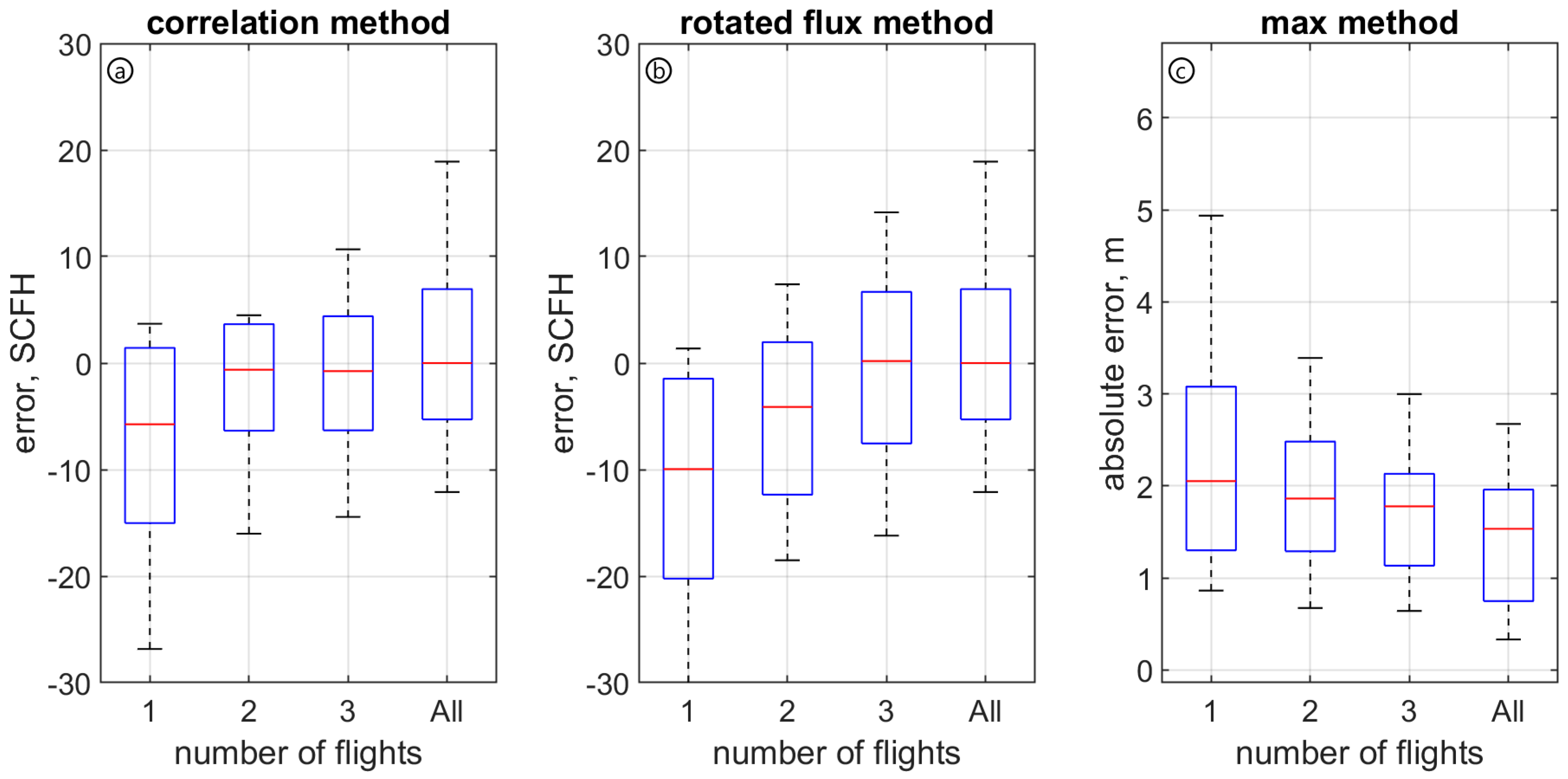
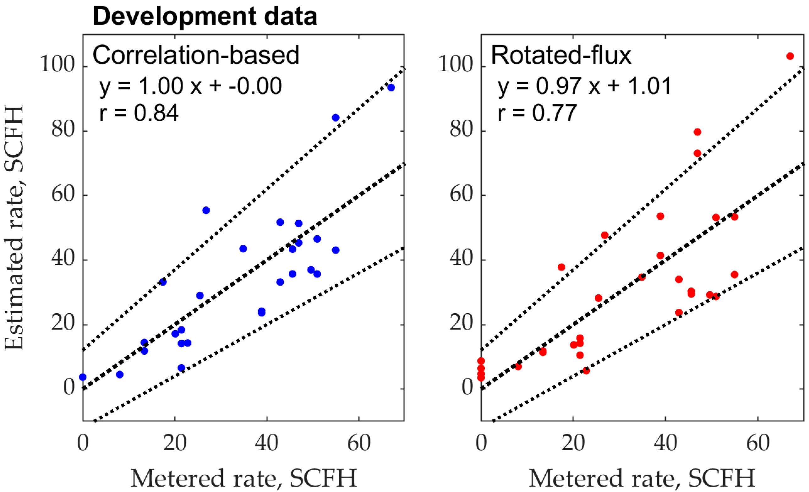
4.2. Leak Detection and Quantification

Two leak rate quantification algorithms were also developed as described in Section 3.2. Both algorithms require parameter choices, which were obtained using the Texas test data. The correlation method’s relationship was specified to yield a result in terms of leak rate (SCFH) with a slope of 1 and intercept of 0, sacrificing slightly on the correlation compared to an unforced fit. For the rotated flux method, the free parameter is identifying which percentile of the crosswind integrated leak rates to use. The 95th percentile was selected to yield a slope and intercept near 1:1. The performance on the test data is shown comparing metered leak rates to the estimates for both algorithms (Figure 9). The correlation-based method has slightly less scatter around the 1:1 line, but there is not a significant difference in performance on the development dataset.

The same algorithms and parameter choices were then applied to the METEC test site to help determine if they are robust. The same style plots are shown (Figure 10). Both methods remained well correlated, with r = 0.84 and 0.85 for the rotated flux and correlation-based methods, respectively. In terms of flow rates, both had only one point outside the error bounds illustrated with dashed lines. Besides being at a completely different site, the leak rates evaluated also tended to be lower than in the development dataset. This may explain why both methods showed a small positive offset, since more weight was placed on measurements near the detection limit of the algorithm, which was intended to be near 6 SCFH. In terms of detection, our results had zero false negatives (all 17 leaks detected) and zero false positives (all 13 zeros correctly identified based on the skewness statistic with a threshold of 1.5). The individual detection results are shown in Figure S4.

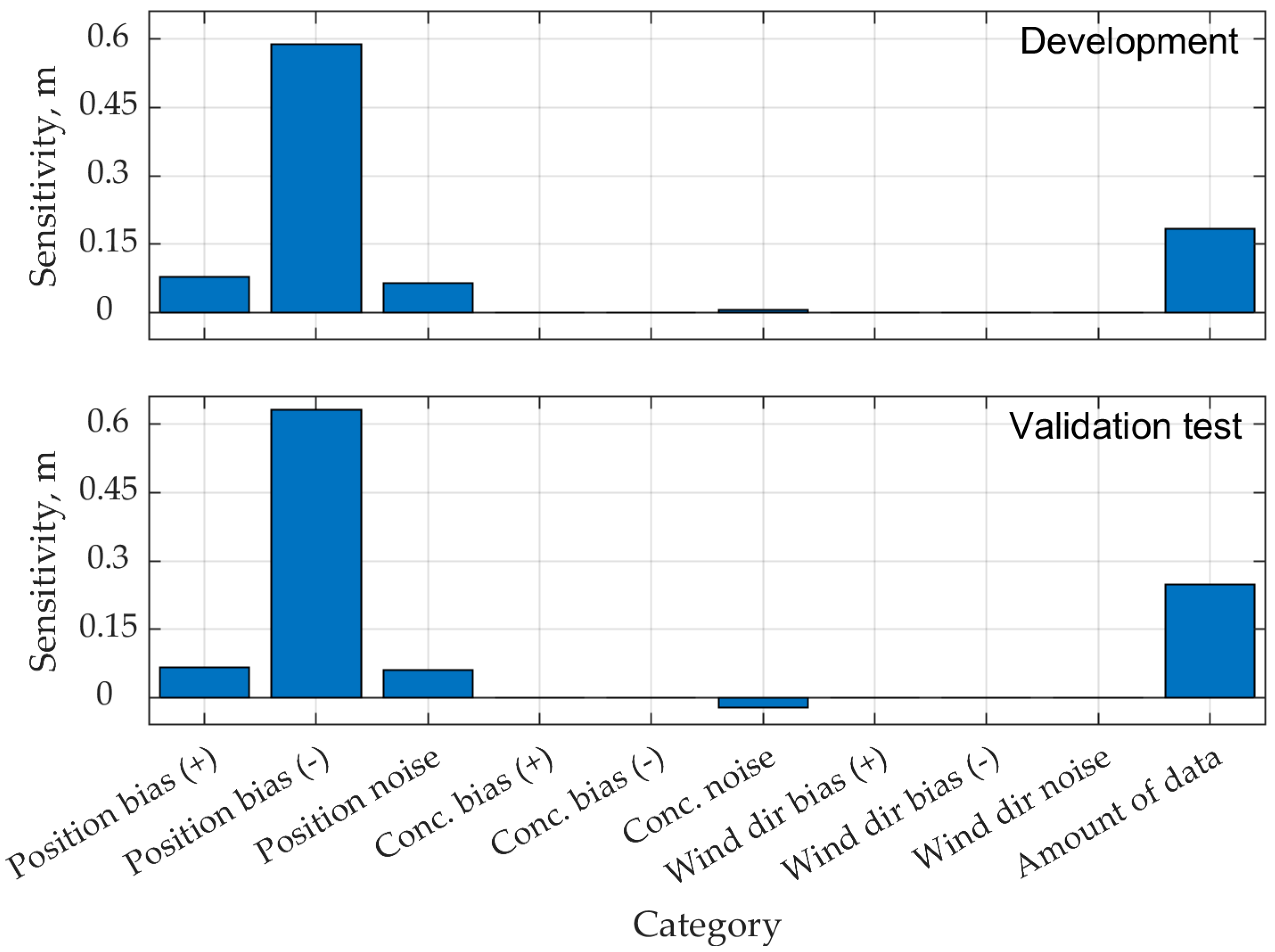
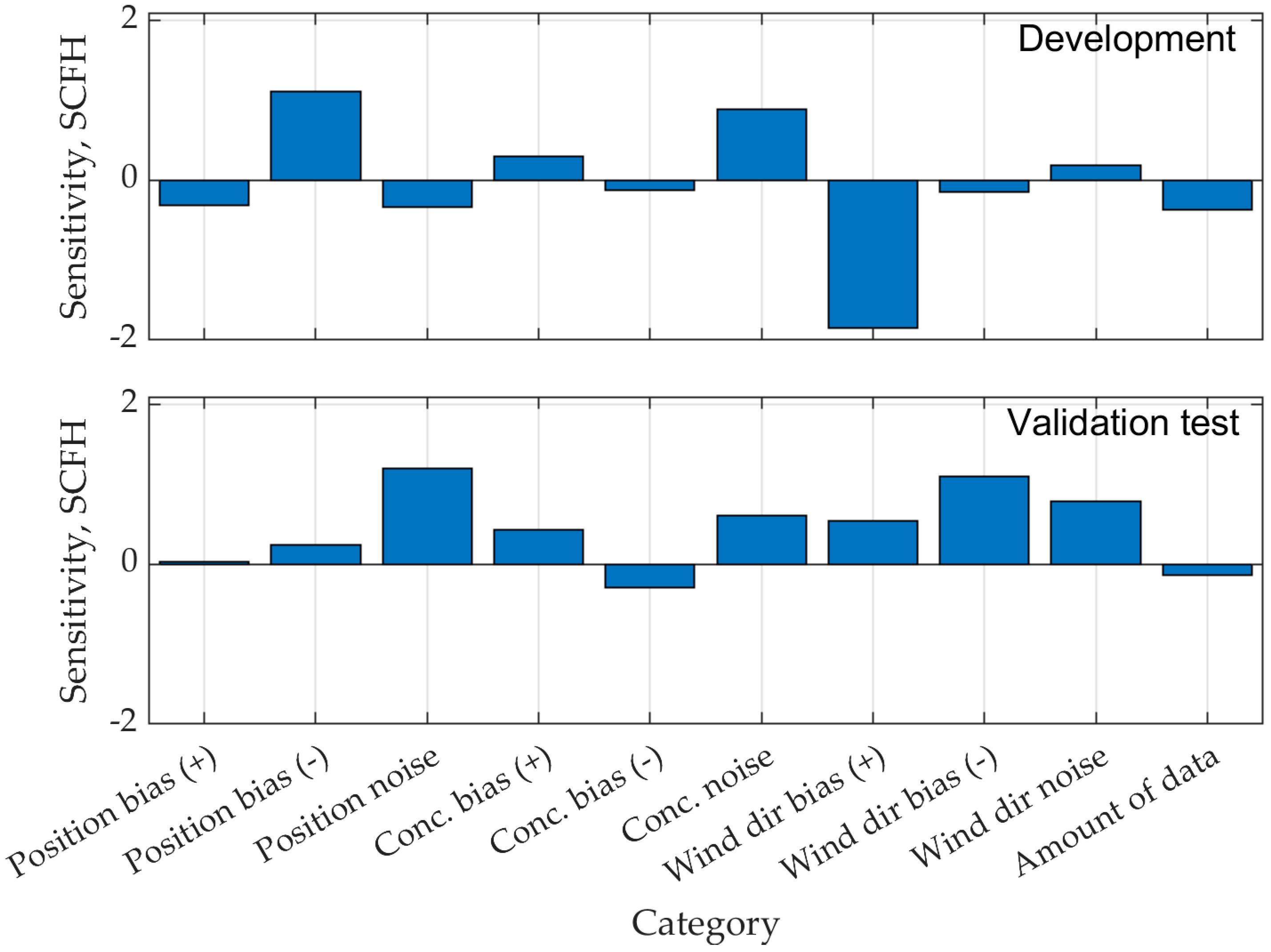
4.3. Component Sensitivity and Uncertainty Analyses

The sensitivity of the algorithms to uncertainty in the input data is now considered. The components include sensor position, methane reading, and wind direction. Sensitivity to each is simulated by individually adding bias and noise to the data shown previously. A fourth category is also considered: namely the amount of flight data used to generate the estimate. Position uncertainty arises from limitations in GPS when used at small scales due to a variety of factors [26,27]. We simulate adding 0.9 m of additional location uncertainty in both x and y. Besides GPS error, position errors can arise from tilt of the RMLD-UAV, causing the laser beam to deviate from pointing straight downward. Concentration bias is modeled here as a multiplicative factor to simulate sensor slope over- or -underestimation. The sensitivity to additive bias (e.g., offset drift) is not shown, since the algorithms are robust against this kind of drift. Wind direction bias could arise if the sensor is not setup to be aligned perfectly with north. Due to the location algorithm being based on the max methane location, concentration errors can also propagate into position errors in other ways besides a bias or normally distributed noise. These include any spurious peaks or if there is optical saturation directly over a leak. There is evidence of the latter, in that for nearly all cases the highest methane reading was obtained slightly downwind of the leak position (Figure S2). Atmospheric conditions can also introduce noise; for instance, downdrafts from the quadcopter rotors or if the methane plume extends above the height of the sensor. These dynamic effects are not directly modeled in this sensitivity analysis, though they are captured in the performance observed in our field data.

Note that the data already contain noise, and so a direct uncertainty budget is not attempted. Still, the sensitivity against reasonable levels of noise helps inform the contributions to the uncertainties in the localization and quantification algorithms. The sensitivity of the max-based localization algorithm is shown and was consistent for the development and METEC datasets (Figure 11). The most noticeable sensitivity is to position bias, which increased the mean error by approximately 0.6 m. This is smaller than the sensitivity expected if there were not already errors in the measurement, where adding 0.9 m to both x and y would result in an error of 1.28 m based on Euclidian distance. Decreasing the amount of data included also increased the error by around 0.2 m. Smaller sensitivities were seen to position noise and concentration noise. The algorithm has no sensitivity to fixed concentration biases or any wind speed or direction noise, since wind is not an input.

The same analysis is now shown for the rotated flux leak rate method (Figure 12). Here, all the data inputs show some sensitivity and there was less consistency between the development and validation datasets. The single largest sensitivity was to wind bias during the development test, which actually showed an improvement compared to when bias was not added. Position bias, wind direction bias, and amount of data all lead to both increases or decreases in mean error, depending on the sign of the noise. This could be the result of compensating for real biases in the input data, or alternatively correcting for unrelated errors. The tendency for positive errors in the validation dataset likely reflects the algorithm not having been specifically optimized for that site. For that site, position noise and wind direction bias were the biggest sensitivities.

The amount of data is now considered further, since it is related to the operation of the RMLD-UAV system. There may be a tradeoff between the number of flights and accuracy obtained, with different applications requiring different levels of accuracy and measurement speed. This is analyzed by using the subset of cases where at least three flights had been conducted. The calculation was repeated using only the first flight, the first two, the first three, and then all the available flights (Figure 13), and without changing the algorithm parameters. The mean number of flights per case was 4. Also note that, for zero leak cases, only one to two flights were conducted, and so the filter by necessity removes these to keep the number of samples consistent. With just two flights included, the correlation method performed comparably to with all flights, except skewing towards low estimates instead of towards high estimates. For the rotated flux method, three flights had the same median as including all flights but a larger spread. For the maximum based location method, there is a continuing trend towards lower errors as the number of flights included increased.

5. Discussion

We return briefly to the two localization and two quantification algorithms presented. The wind-based localization algorithm performed worse than the maxima-based method for the RMLD-UAV flights; however, we noted that the former performed better on the ground-based rotating platform. This may be because the patterns flown were not optimal for the wind-based method since they focused primarily on hovering nearby to the leak. In contrast, it is expected that data taken at least some distance away has a better chance to converge on the leak location as long as peaks can still be robustly distinguished from background. Comparing the two quantification algorithms, the correlation-based algorithm as expected showed a slightly better correlation between metered and estimated leak rates compared to the rotated flux method on the development dataset. Errors for both methods were well distributed around the 1:1 line, with no outliers. However, both methods needed to be tested to see how they perform at sites and wind conditions other than where the parameters were derived. The correlation remained strong (r = 0.85) on the validation dataset, and, despite a positive bias, results with both methods were generally within ±12 SCFH ± 25%. We expect the rotated flux method is likely to be more robust over a wide range of wind conditions, since it uses a mass balance formulation. It is also likely that some wind conditions (specifically, a more-or-less steady, but not necessarily light, wind) will give better results (for both flux and localization) than the light-and-variable winds in which most of our measurements were made.

A unique aspect of this system is that it operates so close to leak sources. Physically, the highest concentration is expected very near to the leak point regardless of atmospheric conditions. This likely reduces the effect of meteorological conditions and also provides an avenue for handling multiple leak sources if they are spatially separated. The trials at METEC have already tested a relatively dense site configuration with three pieces of equipment per 100 m² pad. A typical well pad is larger but often less dense, which can be accommodated by the RMLD-UAV since most time is spent only near where there are leaks. Other benefits are the reduced sensor sensitivity requirements compared to sensors that detect far downwind of the source and the built-in resistance to detecting off-site leaks since enhancements strongly decrease with distance from source (correlation-based method) or generate zero net flux (mass balance-based method). In remote locations, where wind measurements may not be practical, leak detection and localization could still be achieved since the skewness and maximum methods do not require this information. Quantification could use gridded wind products, but with greater uncertainty than if on-site measurements are available. The most common atmospheric approach for quantification in the literature is the application of plume or puff dispersion models in analytical or Bayesian frameworks [28]. Many are tested primarily in simulations rather than real-world experiments, where turbulence fully impacts measurements and there are additional uncertainties (GPS, tilting, separation between the wind ground-based sensor and moving methane sensor, etc.). Here we use instead correlation and mass balance methods. The key innovations were (1) incorporating an algorithm to estimate leak location; (2) using a downwind-crosswind formulation, which may converge more quickly than when not used in this near-source application; (3) and the use of a custom sUAS enabling automated sampling and analysis.

Continuing research will work on refining algorithm performance and testing the system over more leak scenarios and atmospheric conditions. For example, METEC included several tanks but in general tall or densely spaced equipment could pose challenges for the algorithms and sUAS operation. In a long-term deployment setting, knowledge of desirable wind conditions can be leveraged to choose when to target RMLD-UAV measurements. The system will also have to contend with “by design” emissions, such as from a tank or pneumatic controller. Therefore, testing will include multiple or fluctuating sources and longer controlled release scenarios. These could add noise or require longer flight times to accommodate. The algorithms are naturally suited to a probabilistic detection framework, for instance by the gradient from the maximum concentration point or variations in the crosswind integrated flux. More data will help determine if these features can accurately capture periods of greater or lesser uncertainty, and if algorithms parameters can be more tightly optimized.

6. Conclusions

We have demonstrated a simple, data-driven approach for estimating leaks in the natural gas sector using a small unmanned aerial vehicle system. The algorithms are based on flying directly over leaks, in contrast to many techniques which rely on downwind data and dispersion models. After testing multiple algorithms, we find that using the maximum methane location gives a reasonable estimate of leak location, and a downwind-crosswind transformed mass balance algorithm is most consistent for leak quantification. On a blind test on real gas production equipment, localization was achieved within ±1 m for 14 of 17 leak cases. Quantification was more difficult, but estimated leak rates were generally within ±12 SCFH ± 25% of metered values and there were no false positives or negatives, which is important for deployed systems. The greatest uncertainties were ascribed to sensor position uncertainty, concentration noise, and wind direction based on a sensitivity analysis. The algorithms described could form the basis of a continuous monitoring system helping to capture a large fraction of emissions, allowing timely repair and reduction of atmospheric impact from gas leakage.

References

1. Saunois, M.; Bousquet, P.; Poulter, B.; Peregon, A.; Ciais, P.; Canadell, J.G.; Dlugokencky, E.J.; Etiope, G.; Bastviken, D.; Houweling, S.; et al. The global methane budget 2000–2012. Earth Syst. Sci. Data 2016, 8, 697–751. [Google Scholar] [CrossRef] [Green Version]
2. Turner, A.J.; Jacob, D.J.; Benmergui, J.; Wofsy, S.C.; Maasakkers, J.D.; Butz, A.; Hasekamp, O.; Biraud, S.C. A large increase in U.S. methane emissions over the past decade inferred from satellite data and surface observations. Geophys. Res. Lett. 2016, 43, 2218–2224. [Google Scholar] [CrossRef] [Green Version]
3. Zavala-Araiza, D.; Alvarez, R.A.; Lyon, D.R.; Allen, D.T.; Marchese, A.J.; Zimmerle, D.J.; Hamburg, S.P. Super-emitters in natural gas infrastructure are caused by abnormal process conditions. Nat. Commun. 2017, 8, 14012. [Google Scholar] [CrossRef] [PubMed]
4. Mayfield, E.N.; Robinson, A.L.; Cohon, J.L. System-wide and Superemitter Policy Options for the Abatement of Methane Emissions from the U.S. Natural Gas System. Environ. Sci. Technol. 2017, 51, 4772–4780. [Google Scholar] [CrossRef] [PubMed]
5. Alvarez, R.A.; Zavala-Araiza, D.; Lyon, D.R.; Allen, D.T.; Barkley, Z.R.; Brandt, A.R.; Davis, K.J.; Herndon, S.C.; Jacob, D.J.; Karion, A.; et al. Assessment of methane emissions from the U.S. oil and gas supply chain. Science 2018, eaar7204. [Google Scholar] [CrossRef] [PubMed]
6. Melvin, A.M.; Sarofim, M.C.; Crimmins, A.R. Climate Benefits of U.S. EPA Programs and Policies that Reduced Methane Emissions 1993–2013. Environ. Sci. Technol. 2016, 50, 6873–6881. [Google Scholar] [CrossRef] [PubMed]
7. Ravikumar, A.P.; Wang, J.; Brandt, A.R. Are Optical Gas Imaging Technologies Effective For Methane Leak Detection? Environ. Sci. Technol. 2017, 51, 718–724. [Google Scholar] [CrossRef] [PubMed]
8. Hanna, S.R.; Young, G.S. The need for harmonization of methods for finding locations and magnitudes of air pollution sources using observations of concentrations and wind fields. Atmos. Environ. 2017, 148, 361–363. [Google Scholar] [CrossRef]
9. Hirst, B.; Jonathan, P.; González del Cueto, F.; Randell, D.; Kosut, O. Locating and quantifying gas emission sources using remotely obtained concentration data. Atmos. Environ. 2013, 74, 141–158. [Google Scholar] [CrossRef] [Green Version]
10. Yacovitch, T.I.; Herndon, S.C.; Pétron, G.; Kofler, J.; Lyon, D.; Zahniser, M.S.; Kolb, C.E. Mobile Laboratory Observations of Methane Emissions in the Barnett Shale Region. Environ. Sci. Technol. 2015, 49, 7889–7895. [Google Scholar] [CrossRef] [PubMed]
11. Rella, C.W.; Tsai, T.R.; Botkin, C.G.; Crosson, E.R.; Steele, D. Measuring Emissions from Oil and Natural Gas Well Pads Using the Mobile Flux Plane Technique. Environ. Sci. Technol. 2015, 49, 4742–4748. [Google Scholar] [CrossRef] [PubMed]
12. Nathan, B.J.; Golston, L.M.; O’Brien, A.S.; Ross, K.; Harrison, W.A.; Tao, L.; Lary, D.J.; Johnson, D.R.; Covington, A.N.; Clark, N.N.; et al. Near-Field Characterization of Methane Emission Variability from a Compressor Station Using a Model Aircraft. Environ. Sci. Technol. 2015, 49, 7896–7903. [Google Scholar] [CrossRef] [PubMed]
13. Chambers, A.K.; Strosher, M.; Wootton, T.; Moncrieff, J.; McCready, P. Direct Measurement of Fugitive Emissions of Hydrocarbons from a Refinery. J. Air Waste Manag. Assoc. 2008, 58, 1047–1056. [Google Scholar] [CrossRef] [PubMed] [Green Version]
14. Kemp, C.E.; Ravikumar, A.P.; Brandt, A.R. Comparing Natural Gas Leakage Detection Technologies Using an Open-Source “Virtual Gas Field” Simulator. Environ. Sci. Technol. 2016, 50, 4546–4553. [Google Scholar] [CrossRef] [PubMed]
15. Yang, S.; Talbot, R.W.; Frish, M.B.; Golston, L.M.; Aubut, N.F.; Zondlo, M.A.; Gretencord, C.; McSpiritt, J. Detection and Quantification of Fugitive Natural Gas Leaks Using an Unmanned Aerial System. 2018; submitted. [Google Scholar]
16. Frish, M.B.; Wainner, R.T.; Stafford-Evans, J.; Green, B.D.; Allen, M.G.; Chancey, S.; Rutherford, J.; Midgley, G.; Wehnert, P. Standoff sensing of natural gas leaks: Evolution of the remote methane leak detector (RMLD). In Proceedings of the 2005 IEEE Quantum Electronics and Laser Science Conference, Baltimore, MD, USA, 22–27 May 2005; Volume 3, pp. 1941–1943. [Google Scholar]
17. Wainner, R.T.; Green, B.D.; Allen, M.G.; White, M.A.; Stafford-Evans, J.; Naper, R. Handheld, battery-powered near-IR TDL sensor for stand-off detection of gas and vapor plumes. Appl. Phys. B Lasers Opt. 2002, 75, 249–254. [Google Scholar] [CrossRef]
18. Schuyler, T.; Guzman, M. Unmanned Aerial Systems for Monitoring Trace Tropospheric Gases. Atmosphere 2017, 8, 206. [Google Scholar] [CrossRef]
19. Amanatides, J.; Woo, A. A Fast Voxel Traversal Algorithm for Ray Tracing. In Proceedings of the Eurographics ‘87; 1987. Available online: http://www.cse.chalmers.se/edu/year/2012/course/_courses_2011/TDA361/grid.pdf (accessed on 7 July 2018).
20. Hashmonay, R.A.; Yost, M.G. Localizing Gaseous Fugitive Emission Sources by Combining Real-Time Optical Remote Sensing and Wind Data. J. Air Waste Manag. Assoc. 1999, 49, 1374–1379. [Google Scholar] [CrossRef] [PubMed] [Green Version]
21. Foster-Wittig, T.A.; Thoma, E.D.; Albertson, J.D. Estimation of point source fugitive emission rates from a single sensor time series: A conditionally-sampled Gaussian plume reconstruction. Atmos. Environ. 2015, 115, 101–109. [Google Scholar] [CrossRef]
22. Krings, T.; Neininger, B.; Gerilowski, K.; Krautwurst, S.; Buchwitz, M.; Burrows, J.P.; Lindemann, C.; Ruhtz, T.; Schüttemeyer, D.; Bovensmann, H. Airborne remote sensing and in situ measurements of atmospheric CO2 to quantify point source emissions. Atmos. Meas. Tech. 2018, 11, 721–739. [Google Scholar] [CrossRef]
23. Conley, S.; Faloona, I.; Mehrotra, S.; Suard, M.; Lenschow, D.H.; Sweeney, C.; Herndon, S.; Schwietzke, S.; Pétron, G.; Pifer, J.; et al. Application of Gauss’s theorem to quantify localized surface emissions from airborne measurements of wind and trace gases. Atmos. Meas. Tech. 2017, 10, 3345–3358. [Google Scholar] [CrossRef]
24. Albertson, J.D.; Harvey, T.; Foderaro, G.; Zhu, P.; Zhou, X.; Ferrari, S.; Amin, M.S.; Modrak, M.; Brantley, H.; Thoma, E.D. A Mobile Sensing Approach for Regional Surveillance of Fugitive Methane Emissions in Oil and Gas Production. Environ. Sci. Technol. 2016, 50, 2487–2497. [Google Scholar] [CrossRef] [PubMed] [Green Version]
25. Frish, M.B. Systems and Methods for Sensitive Open-Path Gas Leak and Detection Alarm. U.S. Patent 9797798B2, 24 October 2017. [Google Scholar]
26. Parkinson, B.W. GPS Error Analysis. In Global Positioning System: Theory and Applications, Volume 1; Parkinson, B.W., Spilker, J.J., Jr., Axelrad, P., Enge, P., Eds.; American Institute of Aeronautics and Astronautics: Reston, VI, USA, 1996; pp. 469–483. [Google Scholar]
27. Conley, R.; Cosentino, R.; Hegarty, C.J.; Kaplan, E.D.; Leva, J.L.; de Haag, M.U.; Dyke, K. Van Performance of Stand-Alone GPS. In Understanding GPS: Principles and Applications, 2nd ed.; Kaplan, E.D., Hegarty, C.J., Eds.; Artech House: Norwood, MA, USA, 2006. [Google Scholar]
28. Hutchinson, M.; Oh, H.; Chen, W.-H. A review of source term estimation methods for atmospheric dispersion events using static or mobile sensors. Inf. Fusion 2017, 36, 130–148. [Google Scholar] [CrossRef]
Figure 1. Sample data during a controlled release: (a) methane time series; (b) wind vectors shown based on unmanned aerial system (UAS) location (downsampled for clarity); (c) methane concentrations averaged on a regular grid; (d) interpolated methane data. The black ‘x’ indicates the actual leak position. Vertical dashed lines in (a) represent takeoff and landing. Red lines indicate the Remote Methane Leak Detector (RMLD)-unmanned aerial vehicle (UAV) flight tracks.
Atmosphere 09 00333 g001
Figure 2. Case study at Methane Emissions Technology Evaluation Center (METEC) showing the flight procedure and two flights superimposed on one another. The initial flight detected a leak over the tank, which was followed by a second, more focused flight. Red lines indicate the RMLD-UAV flight tracks.
Atmosphere 09 00333 g002
Figure 3. Wind-based location method: Lines projected upwind from high methane points converge on the leak source. The red circle represents the known actual leak location (here 1 m south and 1 m east of center), and the black x shows the system-estimated leak location.
Atmosphere 09 00333 g003
Figure 4. Maxima-based location method: The highest methane concentration is seen slightly southwest of the rightmost separator, which is flagged as the probable leak location, where right corresponds with east and up with north. Here, the location of the maximum methane on this interpolated grid is shown with a triangle. This is shown in comparison to the real leak location designated with a square. Red lines indicate the RMLD-UAV flight tracks. The dominant wind direction was measured to be southeasterly.
Atmosphere 09 00333 g004
Figure 5. Components of the correlation-based quantification method: flow rate is derived from the combination of (a) peak methane (ppm-m) versus known flow rate (SCFH); (b) peak methane versus wind speed, here shown separately for illustration and with the linear regression in (a) forced through background. The combined relationship, with refinements described in the text, is shown in Figure 9. For (a), regression yielded (±2 σ) a slope of 9.94 ± 4.78 ppm-m SCFH−1 and intercept of 35 ± 170 ppm-m. For (b), the coefficients were 615.6 ± 243.9 ppm-m m s−1 and 71.5 ± 144 ppm-m.
Atmosphere 09 00333 g005
Figure 6. Crosswind-integration rate method: (a) individual measurements after rotation; (b) gridded interpolation of a; and (c) crosswind integrated flux. The horizontal dashed line in (c) indicates the estimated leak rate.
Atmosphere 09 00333 g006
Figure 7. Performance in estimating leak position on the Texas controlled release dataset, using the (a) wind back-projection and (b) maximum methane-based methods described in Section 3.1. Absolute errors are shown for both methods.
Atmosphere 09 00333 g007
Figure 8. Performance in estimating leak position evaluated at METEC using (a) the wind back-projection and (b) maximum methane-based methods described in Section 3.1, and (c) estimates snapped to the nearest grid cell containing equipment. The combined method was within ±1 m for 14 of 17 cases.
Atmosphere 09 00333 g008
Figure 9. Leak rate performance using the (left): correlation-based method and (right): rotated-flux method for 33 scenarios. Dashed lines represent the 1:1 relationship and bounds for ±12 SCFH ±25%. The correlation-based method is forced though 0 for the development dataset as described in the text.
Atmosphere 09 00333 g009
Figure 10. Quantification results during a controlled release validation experiment. The colors reflect the three different well pads (Pad 1: green, Pad 2: red, Pad 3: blue).
Atmosphere 09 00333 g010
Figure 11. Sensitivity analyses for the maximum-based localization method. The y-axis here represents the difference in mean error between the data with and without added noise. Position bias: +/−0.9 m offset to both x and y; position noise: added normally distributed noise (μ = 0 m, σ = 0.3 m); concentration bias: ×/÷1.05x, concentration noise: added normally distributed noise (μ = 0 ppm-m, σ = 5 ppm-m), wind direction bias: +/−25 degrees, wind direction noise: added normally distributed noise (μ = 0 deg., σ = 5 deg.), amount of data: randomly exclude half of the data.
Atmosphere 09 00333 g011
Figure 12. Sensitivity analyses for the rotated flux leak rate method. The same assumptions were applied as in Figure 11.
Atmosphere 09 00333 g012
Figure 13. Effect on the number of flights on leak estimation accuracy, including quantification with the (a) correlation-based method and (b) rotated flux method, and localization with (c) the methane maximum method. On the x-axis is the number of flights included (1, 2, 3, or all flights available). The dataset includes all cases from Texas and METEC where at least 3 flights was available. The red line indicates the median, blue box the 25th and 75 percentiles, and dashed lines the 10th and 90th percentiles.
Atmosphere 09 00333 g013