A Statistical Parameter Correction Technique for WRF Medium-Range Prediction of Near-Surface Temperature and Wind Speed Using Generalized Linear Model

Department of Research and Development, National Center for AgroMeteorology, Seoul 08826, Korea
*
Author to whom correspondence should be addressed.
Atmosphere 2018, 9(8), 291; https://doi.org/10.3390/atmos9080291
Submission received: 12 June 2018
/
Revised: 18 July 2018
/
Accepted: 23 July 2018
/
Published: 27 July 2018
(This article belongs to the Special Issue Weather and Climate Change Challenges in Agricultural and Forest Meteorology)
Abstract
:A statistical post-processing method was developed to increase the accuracy of numerical weather prediction (NWP) and simulation by matching the daily distribution of predicted temperatures and wind speeds using the generalized linear model (GLM) and parameter correction, considering an increase in model bias when the range of the prediction time lengthens. The Land Atmosphere Modeling Package Weather Research and Forecasting model, which provides 12-day agrometeorological predictions for East Asia, was employed from May 2017 to April 2018. Training periods occurred one month prior to and after the test period (12 days). A probabilistic consideration accounts for the relatively short training period. Based on the total and monthly root mean square error values for each test site, the results show an improvement in the NWP accuracy after bias correction. The spatial distributions in July and January were compared in detail. It was also shown that the physical consistency between temperature and wind speed was retained in the correction procedure, and that the GLM exhibited better performance than the quantile matching method based on monthly Pearson correlation comparison. The characteristics of coastal and mountainous sites are different from inland automatic weather stations, indicating that supplements to cover these distinctive topographic locations are necessary.
1. Introduction
Agricultural and forest management are greatly affected by weather and climatic conditions, which can be significant during certain time periods. Weather forecasts for agriculture and forestry sectors should be able to provide medium-range and long-range weather information in the highest possible resolution. For example, the medium-range prediction of minimum temperature and wind speed by a model is very important for classifying frost occurrence and frost-free days [1], and for taking appropriate measures in advance. The National Center for Agro-Meteorology (NCAM) in Korea developed the Land Atmosphere Modeling Package (LAMP) version 1.0 [2] through a series of preliminary studies [3,4], with support from the Korea Meteorological Administration (KMA). Its purpose is to enable user-customized agricultural and forest management by linking users with appropriate decision support tools and diverse applied models for drought, flood, landslide, crop growth, disease, insect pest, etc. The NCAM–LAMP package consists of two components: (1) a Weather Research and Forecasting (WRF) modeling system coupled with a Noah-Multiparameterization (Noah-MP) land surface model (LSM); and (2) offline, independently driven, and one-dimensional LSMs optimized for individual sites. Within the LAMP, the WRF/Noah-MP system produces seven or more days of agricultural and forest weather forecast data with a high resolution of less than 1 km. This agrometeorological model product is being offered as a new service of the NCAM since 2017.
The NCAM WRF/Noah-MP medium-range prediction system is the first operational numerical modeling system dedicated to agrometeorological services in Korea. The NCAM’s first aim for this year is to evaluate and increase the prediction accuracy of the coupled WRF/Noah-MP system. Similar to all numerical modeling systems, it has a high prediction skill within a short time scale. However, it has limited predictability over time. To overcome these limitations, we have attempted to reduce the error in the current model by employing statistical techniques to reduce the bias between LAMP WRF medium-range prediction and automatic weather station (AWS) temperature and wind speed observations.
Bias corrections to numerical weather prediction (NWP) have been studied using various techniques. The most general method increases accuracy using a varied model ensemble. Representatively, there are lagged average forecasting (LAF) [5], which combines the same NWP model operating with various space–time intervals, and super-ensemble [6,7], which combines varied NWP models by assigning them various weights. These ensemble techniques have been applied in many studies, including Matsueda et al., Zhao et al., Pistoia et al., and Hwang et al. [6,7,8,9,10]. However, the technique is time and computational resource intensive, because using several NWP models requires numerous calculations and high execution speed.
As an alternative, studies on statistical bias correction using a single NWP model have been conducted. Glahn et al. [11] corrected the predicted precipitation and temperature by configuring Model Output Statistics (MOS), which consider the linear relationship between predicted and real values. In a subsequent study, Lorenz [12] observed relationships other than linear ones and established a nonlinear MOS that showed better performance than the simple linear MOS. Based on these studies, MOS using a linear regression [13,14,15] and artificial neural network [16,17], the generalized additive model (GAM) [18], and nonlinear transformation [19] have been used for temperature bias corrections. Seo et al. [20] developed an MOS model to correct daytime maximum/minimum temperature, applying it to the KMA’s Global Data Assimilation. In contrast, wind speed has been corrected differently due to its skewness. Odo et al. [21] observed that the wind speed in Nigeria formed a Weibull distribution. Kim et al. [22] found that the wind speed in South Korea has a nearly log-normal distribution, and devised a log-transformed linear regression. Zamo et al. [23] corrected the wind speed in France using a GAM, which is semiparametric and nonlinear as well.
However, MOS is limited because it identifies a statistical relationship based on predicted and real values using long-term data, while operational NWP models usually have short-term period data that vary. There is a danger of distortion while using a single MOS because when the NWP model changes in configuration or physics, statistical correlations between the prediction and the observation also change, which damages consistent relationships. However, the MOS based on short-term data can consider abnormal or abrupt phenomena, such as typhoons. To overcome the limitations of deterministic methods, probabilistic methods have been proposed. Piani et al. [24,25] corrected the predicted daily temperature means with the observation data, applying the same correction to the daily maximum/minimum temperatures using 12 MOS. Importantly, this method considers various relationships between the predicted and real values, and stochastically complements MOS. However, the disadvantage of this technique is that the predicted value is the only explanatory variable in MOS, and lacks a bias correction for daily difference.
For the above reasons, we propose in this paper a method to correct the daily distribution of the predicted near-surface temperature and wind speed from LAMP WRF to KMA AWS. LAMP WRF provides 12-day predictions with three to four-day intervals. It does not have prior information because it was produced after March 2017. To minimize distortion from short-term MOS, ensembles with variables other than the predicted ones were used to correct individual daily distributions. Using the corrections, the cumulative probability values of the predicted data were applied to the corrected distribution to reflect the daily difference for a specific time-site that cannot be considered by a single MOS.
2. Data and Methodology
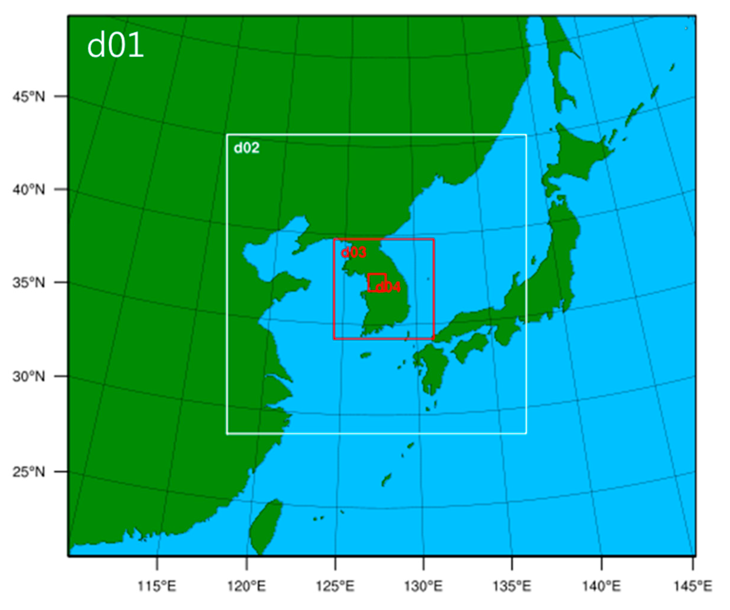
The LAMP WRF medium-range prediction data for model domain 3 (D03) from May 2017 to April 2018 were used. More detailed information on the model domain and physical parameterization is presented in Figure 1 and Table 1. We compared the 2-m temperature and 10-m wind speed prediction data for the location closest to AWS, considering them as the estimated values for that AWS, with the real observation data used to quantify the magnitude of the bias. Wilcke et al. [26] stated that correction biases mainly occur due to low quality observational data. Therefore, minimizing topographic differences between the observation and LAMP grid data was required. AWS sites with height differences of less than 500 m from the model terrain height were selected. Observations at a diurnal temperature range of below 5 °C or above 30 °C were considered unrealistic and removed as missing values. This led to a total of 628 selected sites with a horizontal resolution of 8.8 km. The LAMP-predicted values are affected by both the time elapsed from the initial time and the month (season), displaying differences in prediction patterns. Considering this characteristic, we divided the LAMP prediction length into 12 days so that 12 statistical models corrected the entire WRF model prediction. We set 69–91 h and 261–283 h (from 06 LST on the previous day to 04 LST) from the initial time as the test time slots (Figure 2a). These two time periods were selected since they can be regarded as short and medium-range prediction limits, respectively, from an operational point of view of NWP at KMA. Moreover, our bias correction scheme exhibits a stable and reasonable performance for other prediction hours (e.g., 189–211 h), as well as most of the months and sites (figure not shown).
The correction was based on the assumption that the daily mean distribution of temperature was close to Gaussian, while the distribution of wind speed was close to log normal. Moreover, it was assumed that the daily distribution of the two variables asymptotically followed Gaussian. The distribution consists of two parameters: location and scale. By correcting these parameters, the daily LAMP WRF distributions are corrected to the daily AWS distributions. Assuming that the daily temperature means are also close to a Gaussian distribution, the location parameter was corrected using a simple generalized linear model (GLM), which takes the daily AWS mean as a response variable. The correction of the wind speed parameter was carried out differently because of its skewness. To correct the wind speed parameter, log transformation of the wind speed was used. Variables that show high correlations with observations, such as longitude, latitude, altitude, and daily LAMP variations, were used as explanatory variables in GLM MOS equations to correct each time slot. Individual GLM MOS members can show uncertainty in predicting the relationship between NWP and observational data because of the short-term training period. Therefore, the simple average ensemble, considering average relationships between predictor and explanatory variables, complemented such uncertainty by combining all of the MOS member results after each MOS was generated. The scale parameter was corrected in a manner similar to that of the location parameter. However, the corrected location parameter was added as the explanatory variable to remove unrealistic outputs when the two parameters are corrected separately. The distribution characteristics of temperature and wind speed vary depending on the season and the model integration time. Therefore, prediction data far from the current month are not representative of the bias of the current day. Hence, the data period for MOS training was set from one month prior to and after each dataset, with the test period being from May 2017 to April 2018. As the training and test data are independent, the performance of the GLM MOS model can be approximately verified.
The final form of the MOS proposed in the study is as follows:
Here, the temperature location parameter MOS are represented in Equations (1)–(4), while the scale parameter MOS for the same variable are shown in Equations (5)–(7). The wind speed location parameter MOS are shown in Equations (8)–(11), while the scale parameter for wind speed MOS are seen in Equations (12)–(14). Then, = temperature average, = temperature variation, = predicted temperature average, = predicted water vapor mixing ratio at 2 m (Q2), = predicted soil temperature (TSLB), = observed altitude, = grid point altitude, = latitude, = longitude, = predicted temperature variation, = average temperature obtained from the correction location parameter ensemble, and ) = coefficients corresponding to each temperature MOS variable. Finally, = wind speed average, = wind speed variation, = predicted wind speed mean, = predicted planetary boundary layer height (PBLH), = predicted leaf area index (LAI), = observed altitude, = latitude, = longitude, = predicted wind speed variation, = average wind speed that comes from correction location parameter ensemble, and ) = coefficients corresponding to each wind speed MOS variable.
Variations in sunshine duration change the cumulative probability value corresponding to the daily distribution. Therefore, the cumulative probabilities of the observed values at particular times on various dates also differ. Assuming that LAMP WRF reflects the sunshine variation characteristics, is set as the final correction that satisfies for a predicted value after calculating the cumulative probabilities for each predicted time slot on various days. Equations (15) and (16) are used assuming that the observed and predicted distributions are Gaussian, which is a theoretical distribution. One potential concern is that the wind speed output derived can be a negative value, which is not possible in reality. Therefore, additional post-processing is carried out to change negative values to 0. In the form below, = observed temperature or wind speed value for each site on a given date and time, where m = temperature or wind speed location parameter at each site on a given date, and = temperature or wind speed scale parameter at each site on a given date.
3. Results and Discussion
3.1. Temperature
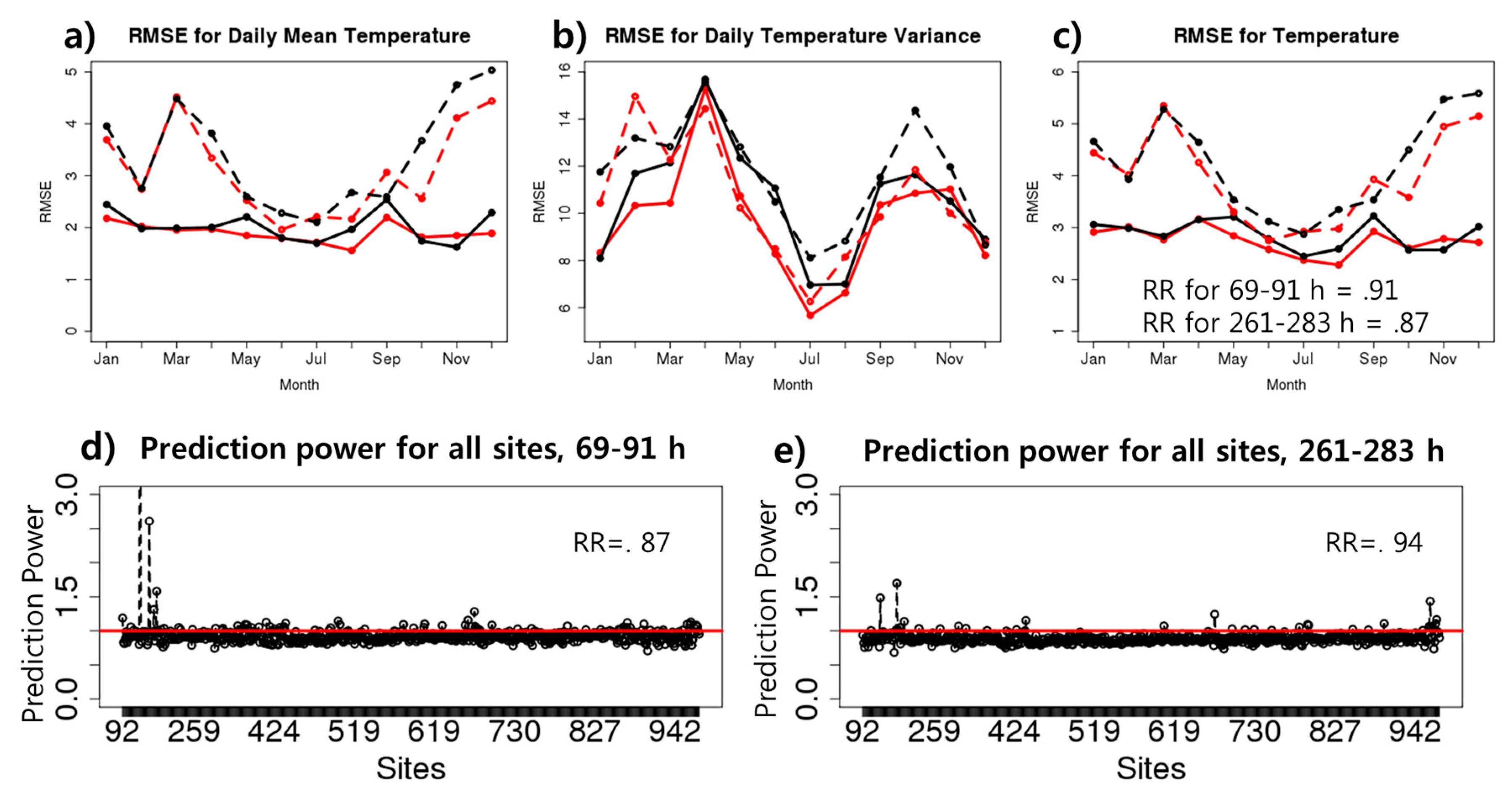
We evaluated the hourly predicted data from LAMP for the test period from May 2017 to April 2018 at 628 sites. Figure 3a shows a comparison of the mean root mean square error (RMSE) for the corrected location parameter. For the 69–91 h time range, the RMSE for the corrected data were lower after correction, except for October and November. In particular, the effects of correction were noticeable in September, December, and January, with large biases before the correction, compared with other months. For the 261–283 h time range, the effects were noticeable in October, November, and December. Figure 3b is a comparison of the mean RMSE for the scale parameter using the bias corrected with the location parameter. Compared with the location parameter, there was a large fluctuation in estimating the scale parameter, which disturbed the bias correction performance. For 69–91 h, a correction effect was observed, except for November. Similarly, for 261–293 h, effects were observed in all of the months except February. Biases in the corrected scale parameter increase for several months due to a lack of information explaining the variation in and shortage of past experience data. Therefore, further evaluations are required in the future. Figure 3c shows the correction result for entire hourly predicted LAMP data using the distribution corrected with the location and scale parameters. For 69–91 h, the corrected RMSE values were lower than the uncorrected data, except for October and November. However, the bias correction performance appeared stable, as the differences between the corrected and uncorrected data RMSE values for the two months appeared to be small. The 261–283 h range showed a decrease in the RMSE in all of the months except September. Overall, the corrected RMSE values for the 69–91 h range were lower than the uncorrected ones by 9%, while the 261–283 h range also showed a 13% improvement.
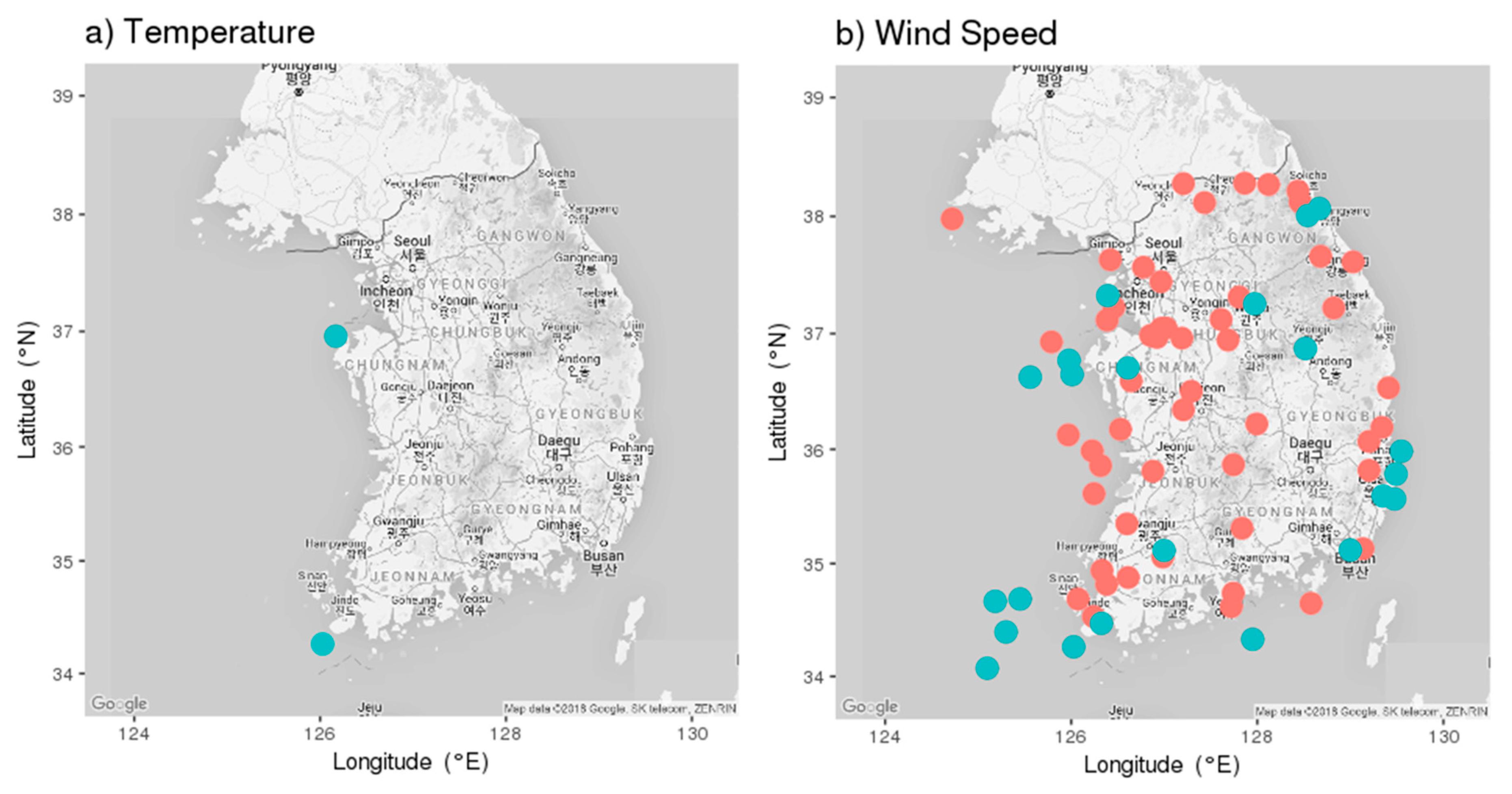
The prediction power evaluates the model predictions for each site. It is the ratio of the corrected mean RMSE to the uncorrected RMSE. Values closer to 0 indicate that the model provides more accurate predictions. Here, i = the entire duration of the test period, and j = the AWS observation site. Figure 3d,e illustrates the prediction powers for 69–91 h and 261–283 h, respectively. There are 87% sites with prediction powers <1 in the 69–91 h range, with 94% in the 261–283 h range. It means that 87% of the 628 sites have a lower corrected RMSE than uncorrected RMSE, while 94% have the same result in the 261–283 h range. In Figure 4a, the highlighted spots are sites with prediction power >1.2, which indicates poor performance on average. These spots are located on the coast or the islands. Since most of the AWS sites used in the corrected model are located inland, sufficient information is not available to explain coastal areas. For example, the land cover representation in the WRF model is not reasonable, with small islands near the coastline being recognized as water in the model, resulting in large thermodynamic differences between the observation and the simulation. Therefore, the established bias correction model is the most appropriate for inland South Korea.
The kriging interpolation method is used to compare the degree of spatial correction inland:
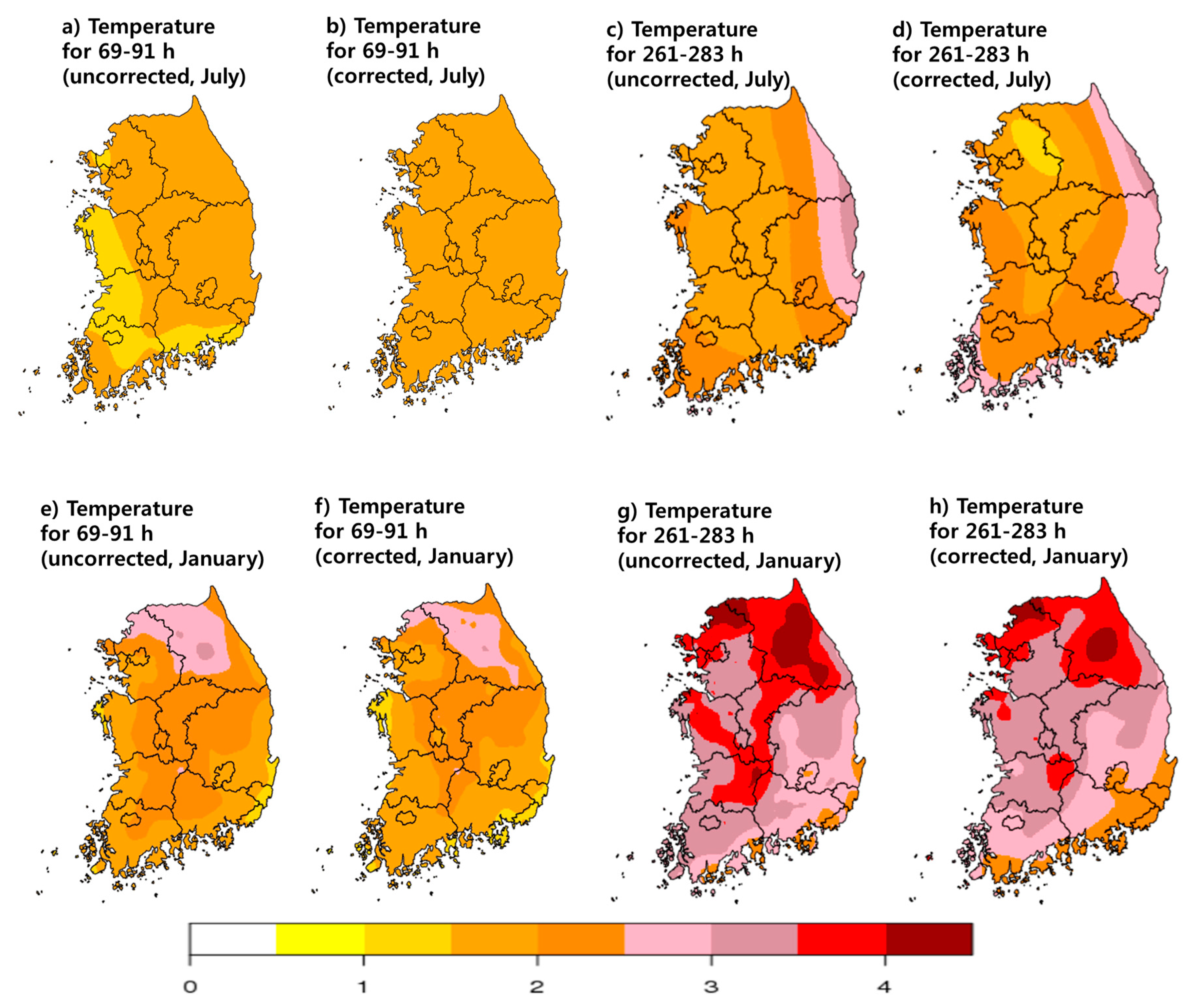
Here, = standard deviation of the uncorrected or corrected error of a grid point, = an observation with locational information, = the weight of to . The details of the interpolation are omitted. Figure 5 shows the spatial distribution of the mean absolute error (MAE) in temperature for July and January. As in Figure 3, the decrease in the RMSE in July (summer) and January (winter) is shown across both time ranges. Overall, the RMSE decreased by 6% in the 69–91 h range, while a 3% increase in the RMSE occurred in the 261–283 h range in July. However, in the 69–91 h range, only 50% of the sites had a lower mean RMSE than uncorrected, which led to a relatively low performance in the southwestern part of the interpolated spatial map, regardless of the total mean RMSE improvement. The maximum value of error among all of the sites in the 69–91 h range was 3.04 in the corrected RMSE, whereas it was 3.34 in the uncorrected one. Thus, it can be concluded that bias correction prevents the predicted temperature from producing a significant error. In the 261–283 h range, 89% of the sites had a lower mean RMSE than the raw value, with a maximum error of 5.64 among all of the sites (5.72 in the uncorrected). In January, the overall RMSE decreased by 9.5% in the 69–91 h range, and by 9.2% in the 261–283 h range. In addition, 69% of the sites had a lower RMSE than the raw value in the 69–91 h range, showing improvement in 78% of the sites in the other time range. The maximum corrected error is 5.16, whereas it is 5.86 in the uncorrected data in the 69–91 h range. In the other time range, the maximum corrected error is 6.65, while the uncorrected is 6.68. In summary, the performance of bias correction in July and January improves the mean of RMSE for most of the sites, and decreases the error ranges.
3.2. Wind Speed
Wind speed was corrected using a method similar to that of temperature. The location parameter correction provided a lower corrected RMSE than the uncorrected RMSE for both time ranges. Specifically, the RMSE of the mean and the variance dropped significantly in July and September, which led to an overall improvement in the RMSE for the 69–91 h time range. While there was some variability in the uncorrected RMSE based on the location and scale parameter, the corrected RMSE was below three for all of the months and time ranges, indicating general stability. There was a significant improvement in the 261–283 h range, where the uncorrected July RMSE was >5, while the corrected RMSE reduced to nearly 2. In summary, the corrected wind speed model provided consistent and accurate results, as indicated by the low corrected RMSE values and small error variations compared to the uncorrected values. Figure 6c shows all of the hourly predicted wind speed data, displaying an improvement for most of the months and time ranges. Comparing the uncorrected and corrected RMSE values, the RMSE improved by 43% for the 69–91 h time range and 55% for the 261–283 h range. As seen in Figure 6d,e, 84% of the sites in the 69–91 h range had prediction powers <1, while 93% of the sites in the 261–283 h range had a lower mean RMSE than the uncorrected data. In Figure 3b, sites with prediction powers >1.2 are marked, showing that most were located in coastal, mountainous, and island environments, which are similar to the temperature correction results. These areas have topographic conditions that are different from inland areas. Therefore, the bias correction for these geographical features should be pursued in the future after collecting sufficient information from these sites.
Figure 7 illustrates the spatial distribution of wind speed results, indicating an improvement in the MAE for the two time ranges in January and July. More significant improvements were observed in July. While 90% of the sites showed lower corrected mean RMSE than the uncorrected data in the 69–91 h time range, 97% of the sites showed an improvement in the 261–283 h range. However, the maximum error value was higher than that for the uncorrected data, requiring further studies. The overall RMSE improvement showed a 59% decrease in the 69–91 h range, and an 88% decrease in the 261–283 h range in July. In January, 60% of the sites showed an improvement in the 69–91 h range, while 80% of sites showed an improvement in the 261–283 h range. The maximum error of the sites was reduced from 13.8 to 6.8 in the 69–91 h range, while the value became slightly higher in the 261–283 h range. However, it was small and could be neglected. In summary, the bias correction of wind speed in January and July significantly improved the mean RMSE in most of the sites, as well as the total RMSE.
3.3. Performance of Bias Correction and Discussions
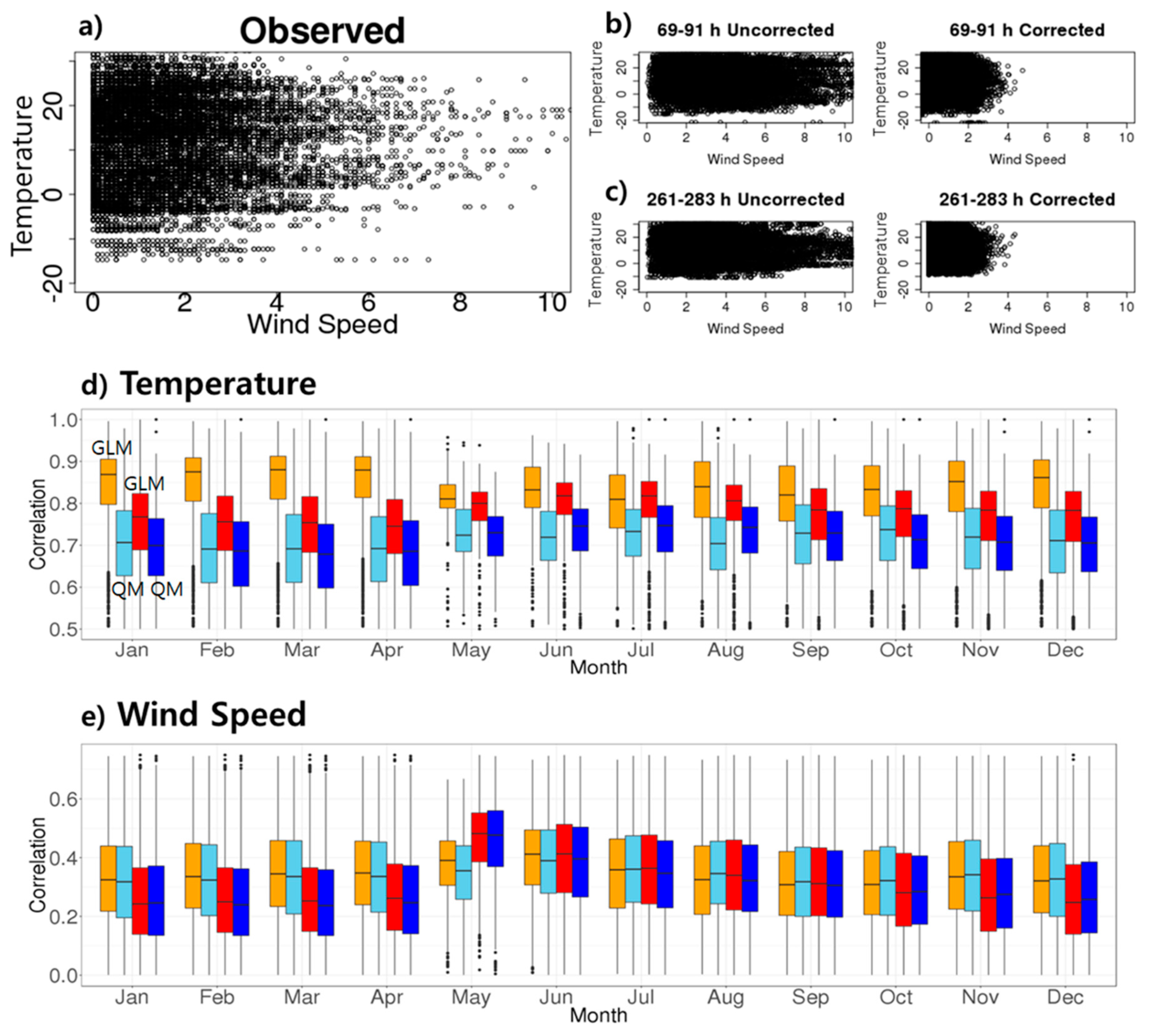
The evaluation of physical consistencies of temperature and wind speed is shown in Figure 8a–c. While the uncorrected model results tended to overpredict the wind speed, the scale of correction of wind speed reduced, indicating that the corrected model results had consistencies similar to the real observation. Nevertheless, the correction had a tendency of not capturing strong winds over 4 m s−1.
Cumulative probabilities calculated from the LAMP WRF daily distributions were used to substitute for the cumulative probabilities from the daily distributions corrected using the parameter MOS ensembles. The GLM-based bias correction is similar to the quantile matching (QM) algorithm [26,27], as the cumulative probabilities from the uncorrected model are used in the corrected distribution. The difference is that the bias correction used in this study assumed theoretical distribution for the daily distribution, while QM considered the empirical distribution for the entire training period. Figure 8d,e shows a comparison of Pearson correlation between the GLM-based bias correction and QM. The training data used in QM correction was the same as those used in the GLM bias correction, considering seasonal differences. With regard to temperature, our bias correction showed better performance across all of the months than QM. Similarly, wind speed also showed better performance. However, it had lower correlation than QM from August to December in the 69–91 h range. The bias correction using GLM showed better performance in predicting across a wide range of regions, reducing the time required. However, it does not necessarily mean that QM lacks correction skills, because QM is focused on a small space. QM is usually applied for every single station separately. The aim of this study was to correct the entire inland area of South Korea. Therefore, we assumed the area as one block [27], and evaluated the performance between QM and the bias correction that we developed.
The general problem of bias correction in this and similar studies is referred to as the “Mars problem” by Maraun and Widmann [28]. Theoretically, we may obtain data from Mars, fit the data to some place on Earth, and obtain a perfect validation score. However, there is probably no physical correlation between the phenomena seen by the model and those observed in reality. Maraun and Widmann point out the dangers of cross-validation of bias-corrected climate simulation, mainly due to the realization of internal variability in the observations and climate model. For example, badly bias-corrected air temperature on the coast may change local atmospheric circulations such as sea breezes due to the change in the horizontal temperature contrast between the land and sea. To clearly address this issue, some geophysics and thermodynamics calculations would be required. However, this is beyond the scope of the present research, and incidentally does not impact the results obtained from the above method, as it is not assimilated in the WRF simulation [29]. On the other hand, the LAMP WRF model deals with medium-range (12-day) predictions, which start from the initial model fields, instead of climate projections. During model integration, the possibility of internal instability and uncertainty also gradually increases, while a free-running state can partly or completely occur within the domain. However, in our study, the bias-corrected results of the model variables were not used to update or modify the other related model variables. One of the short-term practical methods to resolve this potential problem in both statistical bias correction and NWP viewpoints is to expand the outermost domain so that the initial state and inflow boundary information is retained as much as possible. Secondly, we need to adopt higher-resolution land-cover and terrain maps to realistically represent coastal and mountainous areas. Thirdly, we must provide the local agrometeorological community and the corresponding users with model verification information on the accuracy of the previous 12-day model prediction on a regular basis. Finally, we can improve the downscaling strategy through a perfect initial/boundary conditions approach (i.e., with the use of ERA-5 or ERA-Interim as the initial/boundary conditions).
4. Summary and Concluding Remarks
Predicted daily distributions from the LAMP WRF/Noah-MP model were corrected to the daily data distributions from the observed sites with the goal of decreasing errors in temperature and wind speed. A Gaussian distribution was assumed, as this is close to the daily distribution of the two measured variables. Using an MOS ensemble that corrects the parameters, we consider multiple relations between the predicted and observational data. Our results show the impacts of both the location and scale parameter corrections, considering their association. Comparing the corrected and the uncorrected RMSE for the location parameter over the 69–91 h and 261–283 h ranges, overall improvements were obtained with only a few excluded months. Similar results were observed when comparing the scale parameter RMSE values before and after correction. Although some exceptions exist with a small magnitude of error, the total RMSE of the corrected prediction is improved compared to the uncorrected LAMP. RMSE improvements for hourly data were observed as a result, while the non-stationarity of errors remained due to the fluctuation error of the uncorrected model, which requires further study.
A comparison of spatial distribution using the kriging interpolation revealed that temperature correction provides the most accurate improvement in inland areas. Wind speed was corrected using the same method as temperature. However, its location parameter was assumed to follow log-normal distribution. The corrected results show significant improvements in the two parameter corrections, which provide more accurate prediction data. Furthermore, we found that, based on the spatial distribution of wind speed, the MAE decreases toward the east and inland. Comparing the temperature/wind speed prediction power for each site tested, most of the sites showed an improvement in the mean RMSE across both of the time ranges. Physical consistency existed between the corrected variables, i.e., temperature and wind speed, as it resembles the observed data more than uncorrected LAMP. Moreover, compared with another bias correction, QM, the Pearson correlation of bias correction using GLM obtains a higher score. This means that the GLM result has more relevance with observational data.
In summary, the method proposed in this study is distinct from prior studies in that it uses a stochastic bias correction with short-term data, reflecting daily differences. We believe that the method may be used in other types of NWP models, as well as NCAM WRF/Noah-MP. Finally, sites at locations that are topography different from the normal inland areas showed a poorer average prediction performance. Investigating the characteristics of these sites should be a priority in the future studies of bias correction.
Author Contributions
S.-J.L. configured and performed the NCAM WRF model predictions; J.J. analyzed and statistically corrected the model results; J.J. and S.-J.L. wrote the paper and both authors contributed to the interpretation of the results.
Acknowledgments
The authors would like to thank the three anonymous reviewers for their valuable comments and thoughtful suggestions to improve the quality of the paper. This work was funded by the Korea Meteorological Administration Research and Development Program under Grant KMI2018-04810. Also, this study was carried out with the support of ‘R&D Program for Forest Science Technology (Project No. 2018119B10-1820-AB01)’ provided by Korea Forest Service(Korea Forestry Promotion Institute).
Conflicts of Interest
The authors declare no conflict of interest.
References
- Kim, Y.; Shim, K.M.; Jung, M.P.; Choi, I. Study on the Estimation of Frost Occurrence Classification Using Machine Learning Methods. Korean J. Agric. For. Meteorol. 2017, 19, 86–92. [Google Scholar]
- Lee, S.-J.; Song, J.; Kim, Y. The NCAM Land-Atmosphere Modeling Package (LAMP) Version 1: Implementation and Evaluation. Korean J. Agric. For. Meteorol. 2016, 18, 307–319. [Google Scholar] [CrossRef] [Green Version]
- Lee, S.-J.; Kim, J.; Kang, M.; Takuri, B.M. Numerical Simulation of Local Atmospheric Circulation in the Valley of KoFlux Observation Site. Korean J. Agric. For. Meteorol. 2014, 16, 244–258. [Google Scholar]
- Song, J.; Lee, S.-J.; Kang, M.; Moon, M.; Lee, J.; Kim, J. Numerical Simulation of High Resolution WRF/Noah-MP in Farmland around Cheongmicheon Stream during the Special Observation Period. Korean J. Agric. For. Meteorol. 2015, 17, 384–398. [Google Scholar] [CrossRef]
- Hoffman, R.N.; Kalnay, E. Lagged average forecasting, an alternative to Monte Carlo forecasting. Tellus 1983, 35, 100–118. [Google Scholar] [CrossRef]
- Matsueda, M.; Kyouda, M.; Tanaka, H.L.; Tsuyuki, T. Daily Forecast Skill of Multi-Center Grand Ensemble. SOLA 2007, 3, 29–32. [Google Scholar] [CrossRef] [Green Version]
- Rixen, M.; Le Gac, J.-C.; Hermand, J.-P.; Peggion, G.; Coelho, E. Super-ensemble Forecast and Resulting Acoustic Sensitivities in Shallow Waters. J. Mar. Syst. 2009, 78, 290–305. [Google Scholar] [CrossRef]
- Zhao, J.; Xu, J.; Xie, X.; Lu, H. Drought Monitoring Based on TIGGE and Distributed Hydrological Model in Huaihe River Basin, China. Total Envrion. 2016, 553, 358–365. [Google Scholar] [CrossRef] [PubMed]
- Pistoia, J.; Pinardi, N.; Oddo, P.; Collins, M.; Korres, G.; Drillel, Y. Development of Super-ensemble Techniques for Ocean Analyses: The Mediterranean Sea Case. Nat. Hazards Earth Syst. Sci. 2016, 16, 1807–1819. [Google Scholar] [CrossRef]
- Hwang, Y.; Han, K.; Kim, C. Coupling and Correction of Multi-model Ensemble. In Proceedings of the Autumn Meeting of Korea Meteorological Society, Busan, Korea, 25–27 October 2017; pp. 408–409. [Google Scholar]
- Glahn, H.R.; Lowry, R. The Use of Model Output Statistics (MOS) in Objective Weather Forecasting. J. Appl. Meteorol. 1972, 11, 1203–1211. [Google Scholar] [CrossRef]
- Lorenz, E.N. An Experiment in Nonlinear Statistical Weather Forecasting. Mon. Weather Rev. 1977, 105, 590–602. [Google Scholar] [CrossRef] [Green Version]
- Massie, R.D.; Rose, M.A. Predicting Daily Maximum Temperatures Using Linear Regression and Eta Geopotential Thickness Forests. Weather Forecast. 1997, 12, 799–807. [Google Scholar] [CrossRef]
- Myoung, J.; Oh, S.; Suh, M. Improvement of Simulated Air Temperature of Regional Climate Model using Linear Regression Method. Clim. Res. 2012, 7, 255–270. [Google Scholar]
- Termonia, P.; Deckmyn, A. Model-inspired Predictors for Model Output Statistics (MOS). Mon. Weather Rev. 2007, 135, 3496–3505. [Google Scholar] [CrossRef]
- Lee, B.; Kang, B. Downscaling GCM Climate Change Output using Quantile Mapping and Artificial Neural Network. In Proceedings of the Korean Society of Civil Engineers, Daegu, Korea, 29–30 October 2008; pp. 1603–1606. [Google Scholar]
- Marzban, C. Neural Networks for Postprocessing Model Output: ARPS. Mon. Weather Rev. 2003, 131, 1103–1111. [Google Scholar] [CrossRef] [Green Version]
- Vislocky, R.L.; Fritsch, J.M. Generalized Additive Models versus Linear Regression in Generating Probabilistic MOS Forecasts of Aviation Weather Parameters. Weather Forecast. 1995, 10, 669–680. [Google Scholar] [CrossRef] [Green Version]
- Bordoy, R.; Burlando, P. Bias Correction of Regional Climate Model Simulations in a Region of Complex Orography. J. Appl. Meteorol. Clim. 2013, 52, 82–101. [Google Scholar] [CrossRef]
- Seo, Y.; Choi, J.; Lee, J.; Jeong, H. Improvement of Statistical Model (MOS) for Supporting Digital Weather Forecast. In Proceedings of the Autumn Meeting of Korea Meteorological Society, Daegu, Korea, 1–2 November 2012; pp. 110–111. [Google Scholar]
- Odo, F.C.; Offiah, S.U.; Ugwuoke, P.E. Weibull Distribution-based Model for Prediction of Wind Potential in Enugu, Nigeria. Adv. Appl. Sci. Res. 2012, 3, 1202–1208. [Google Scholar]
- Kim, H.-J.; Kim, H.; Choi, Y.; Lee, S.; Seo, B. A Statistical Tuning Method to Improve the Accuracy of 1 km × 1 km Resolution Wind Data of South Korea Generated from a Numerical Meteorological Model. Korean J. Appl. Stat. 2011, 24, 1225–1235. [Google Scholar] [CrossRef]
- Zamo, M.; Bel, L.; Mestre, O.; Stein, J. Improved Gridded Wind Speed Forecasts by Statistical Postprocessing of Numerical Models with Block Regression. Weather Forecast. 2016, 31, 1929–1945. [Google Scholar] [CrossRef]
- Piani, C.; Haerter, J.O.; Coppola, E. Statistical Bias Correction for Daily Precipitation in Regional Climate Models over Europe. Theor. Appl. Clim. 2010, 99, 187–192. [Google Scholar] [CrossRef]
- Piani, C.; Weedon, G.P.; Best, M.; Gomes, S.M.; Viterbo, P.; Hagemann, S.; Haerter, J.O. Statistical Bias Correction of Global Simulated Daily Precipitation and Temperature for the Application of Hydrological Models. J. Hydrol. 2010, 395, 199–215. [Google Scholar] [CrossRef]
- Wilcke, R.A.; Mendlik, T.; Gobiet, A. Multi-variable error correction of regional climate models. Clim. Chang. 2013, 120, 871–887. [Google Scholar] [CrossRef] [Green Version]
- Gutiérrez, J.M.; Maraun, D.; Widmann, M.; Huth, R.; Hertig, E.; Benestad, R.; Roessler, O.; Wibig, J.; Wilcke, R.; Kotlarski, S.; et al. An Intercomparison of a Large Ensemble of Statistical Downscaling Methods over Europe: Results from the VALUE Perfect Predictor Cross-validation Experiment. Int. J. Clim. 2018. [Google Scholar] [CrossRef]
- Maraun, D.; Widmann, M. Cross-validation of Bias-corrected Climate Simulations is Misleading. Hydrol. Earth Syst. Sci. Discuss. 2018. [Google Scholar] [CrossRef]
- Lee, S.-J.; Parrish, D.F.; Wu, W.-S.; Park, S.-Y.; Greybush, S.J.; Lee, W.-J.; Lord, S.J. Effects of 2-m Air Temperature Assimilation and a New Near-Surface Observation Operator on the NCEP Gridpoint Statistical-Interpolation System. Asia-Pac. J. Atmos. Sci. 2011, 47, 353–376. [Google Scholar] [CrossRef]
Figure 1.
National Center for Agro-Meteorology (NCAM)–Land Atmosphere Modeling Package (LAMP) Weather Research and Forecasting (WRF)/ Noah-Multiparameterization (Noah-MP) model (version 1.5) domains.
Figure 1.
National Center for Agro-Meteorology (NCAM)–Land Atmosphere Modeling Package (LAMP) Weather Research and Forecasting (WRF)/ Noah-Multiparameterization (Noah-MP) model (version 1.5) domains.

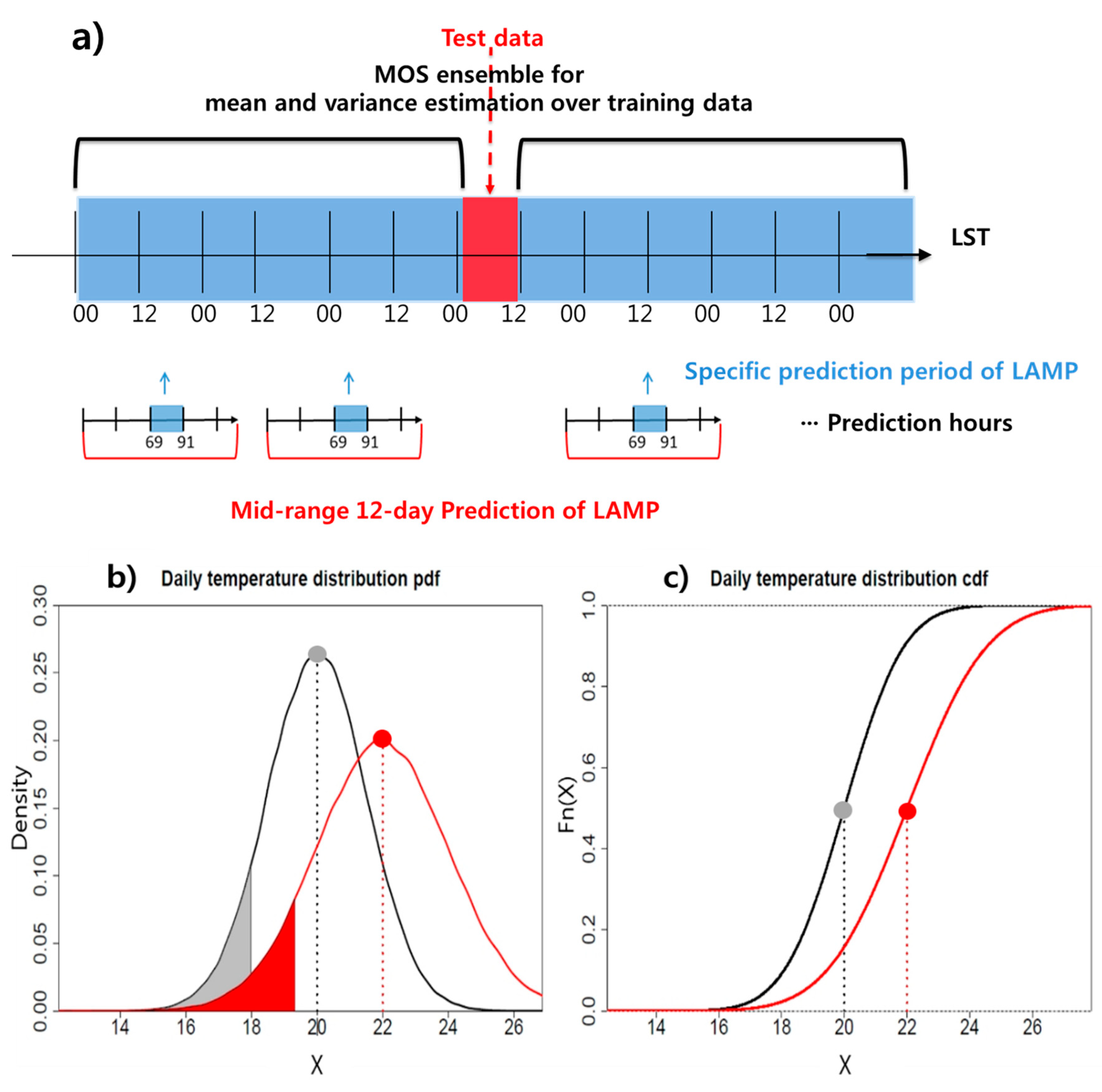
Figure 2.
Bias correction for temperature and wind speed in this study. (a) Diagram of the Model Output Statistics (MOS) ensemble for parameter correction. (b) Probability density functions for daily temperature, and (c) cumulative density functions for daily temperature. The black line distribution is the original LAMP WRF data, i.e., uncorrected prediction, and the red line is the corrected LAMP WRF data. The grey and red regions have the same area. Each grey point is corrected to a red point.

Figure 3.
Bias corrected results for daily temperature. (a) Root mean square error (RMSE) of the daily temperature mean, (b) RMSE of the daily temperature variance, and (c) total temperature RMSE: 69–91 h uncorrected (solid black line), 69–91 h corrected (solid red line), 261–283 h uncorrected (dashed black line), 261–283 h corrected (dashed red line). The ratio of the root mean square (‘RR’) for each time slot is in the middle. The ratio of the mean corrected RMSE to the uncorrected RMSE for each site in (d) 69–91 h and (e) 261–283 h.

Figure 4.
Observation sites with prediction powers >1.2 for (a) temperature and (b) wind speed in the 69–91 h (blue) and 261–283 h (red) ranges.
Figure 4.
Observation sites with prediction powers >1.2 for (a) temperature and (b) wind speed in the 69–91 h (blue) and 261–283 h (red) ranges.

Figure 5.
Spatial distributions of temperature MAEs in July 2017 and January 2018. Results are for (a) uncorrected 69–91 h in July 2017, (b) corrected 69–91 h in July 2017, (c) uncorrected 261–283 h in July 2017, (d) corrected 261–283 h in July 2017, (e) uncorrected 69–91 h in January 2018, (f) corrected 69–91 h in January 2018, (g) uncorrected 261–283 h in January 2018 and (h) corrected 261–283 h in January 2018.

Figure 6.
Bias-corrected results for daily wind speed. (a) RMSE of the daily wind speed mean, (b) RMSE of daily wind speed variance, and (c) total wind speed RMSE: 69–91 h uncorrected (solid black line), 69–91 h corrected (solid red line), 261–283 h uncorrected (dashed black line), 261–283 h corrected (dashed red line). The ratio of root mean square (‘RR’) for each time slot is in the middle. The ratio of mean corrected RMSE to uncorrected RMSE for each site in (d) the 69–91 h range and (e) the 261–283 h range.
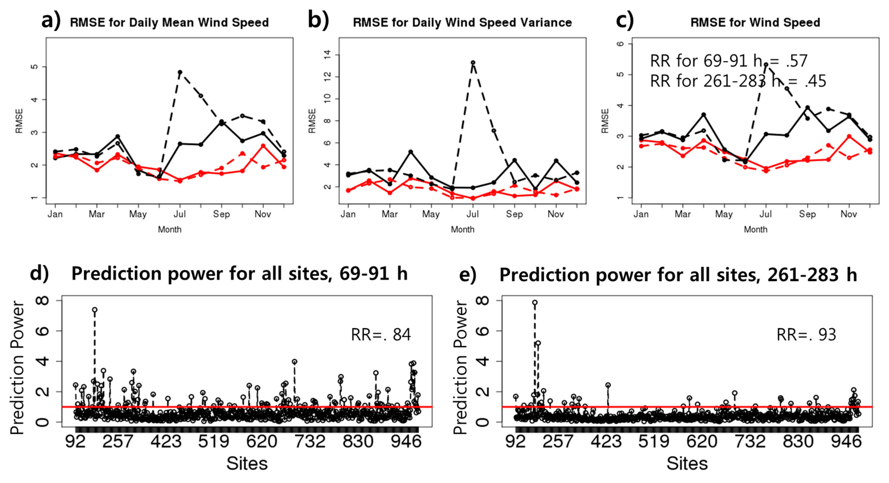
Figure 7.
Spatial distributions of wind speed MAEs in July 2017 and January 2018. Results are for (a) uncorrected 69–91 h in July 2017, (b) corrected 69–91 h in July 2017, (c) uncorrected 261–283 h in July 2017, (d) corrected 261–283 h in July 2017, (e) uncorrected 69–91 h in January 2018, (f) corrected 69–91 h in January 2018, (g) uncorrected 261–283 h in January 2018 and (h) corrected 261–283 h in January 2018.
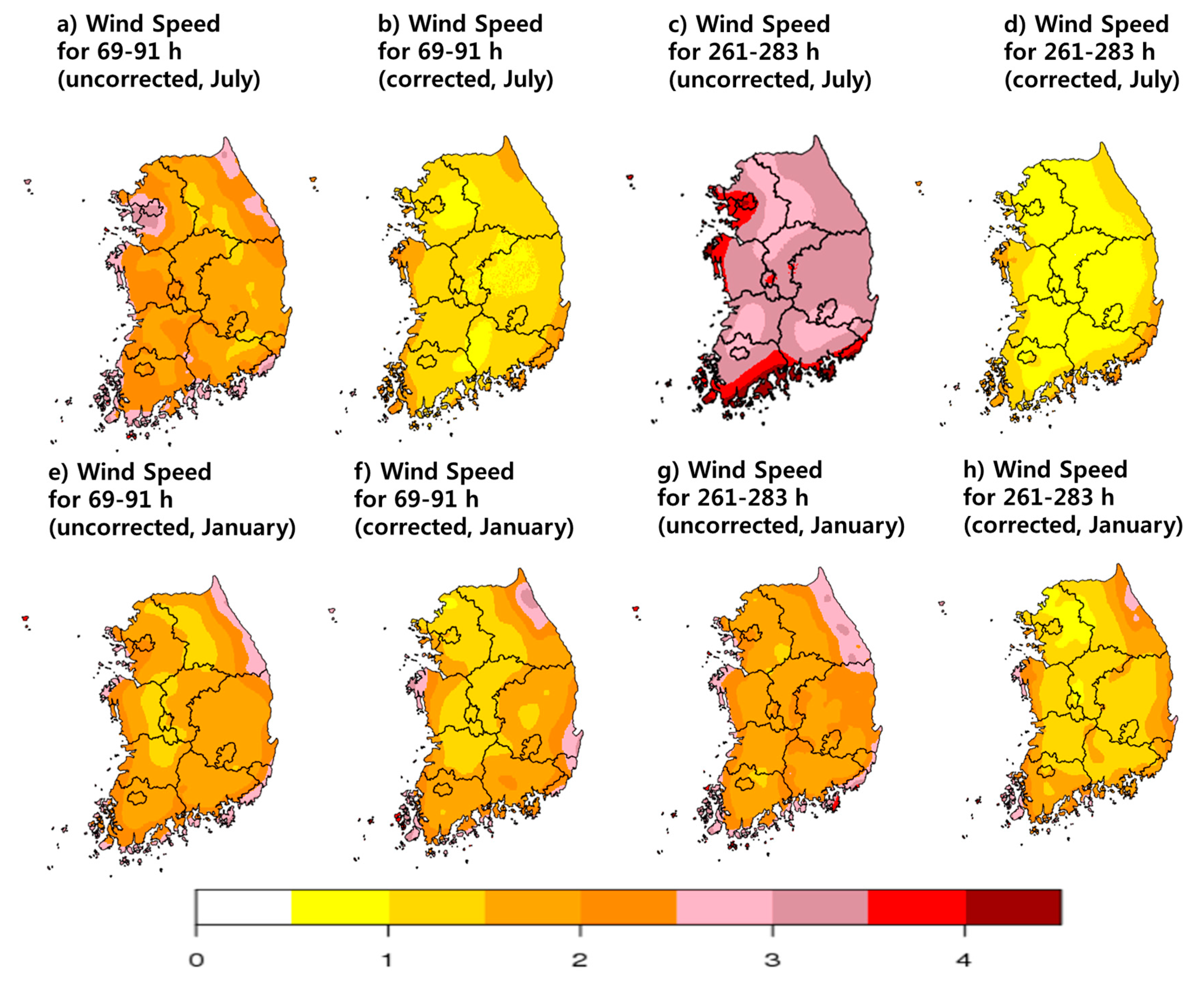
Figure 8.
Scatter plot of temperature and wind speed during the period of May 2017–April 2018 for (a) the observed, (b) the uncorrected and corrected LAMP for 69–91 h, (c) same as (b), but for 261–283 h. (d) and (e) show monthly Pearson correlation of bias correction with a generalized linear model (GLM) and a quantile matching (QM) method in the 69–91 h range (orange for GLM, sky blue for QM) and 261–283 h range (red for GLM, blue for QM).

Table 1.
NCAM–LAMP WRF/Noah-MP model (version 1.5) specifications.
| Domain | Domain 1 | Domain 2 | Domain 3 | Domain 4 |
|---|---|---|---|---|
| (D01) | (D02) | (D03) | (D04) | |
| Model version | WRF–ARW v3.7.1 with Noah-MP land surface model | |||
| Domain size (horizontal resolution) | 175 × 151 | 250 × 250 | 250 × 250 | 130 × 130 |
| (21,870 m) | (7290 m) | (2430 m) | (810 m) | |
| Vertical levels | 39 | 39 | 39 | 39 |
| Topography and land use data resolution (data source) | 30″ | 30″ | 30″ | 1/3″ |
| (USGS) | (USGS) | (USGS) | (Ministry of Environment) | |
| Initial and boundary conditions | UM–GDAPS (Unified Model—Global Data Assimilation and Prediction System at Korea Meteorological Administration) | |||
| Shortwave radiation scheme | Goddard shortwave | |||
| Longwave radiation scheme | RRTM | |||
| Microphysics scheme | WSM6 | |||
| Cumulus scheme | New Kain–Fritsch | New Kain–Fritsch | Off | Off |
| Planetary boundary layer scheme | Shin–Hong | |||
© 2018 by the authors. Licensee MDPI, Basel, Switzerland. This article is an open access article distributed under the terms and conditions of the Creative Commons Attribution (CC BY) license (http://creativecommons.org/licenses/by/4.0/).
Share and Cite
MDPI and ACS Style
Jeong, J.; Lee, S.-J. A Statistical Parameter Correction Technique for WRF Medium-Range Prediction of Near-Surface Temperature and Wind Speed Using Generalized Linear Model. Atmosphere 2018, 9, 291. https://doi.org/10.3390/atmos9080291
AMA Style
Jeong J, Lee S-J. A Statistical Parameter Correction Technique for WRF Medium-Range Prediction of Near-Surface Temperature and Wind Speed Using Generalized Linear Model. Atmosphere. 2018; 9(8):291. https://doi.org/10.3390/atmos9080291
Chicago/Turabian StyleJeong, Jinmyeong, and Seung-Jae Lee. 2018. "A Statistical Parameter Correction Technique for WRF Medium-Range Prediction of Near-Surface Temperature and Wind Speed Using Generalized Linear Model" Atmosphere 9, no. 8: 291. https://doi.org/10.3390/atmos9080291
Note that from the first issue of 2016, this journal uses article numbers instead of page numbers. See further details here.