A Mechanism of the Interdecadal Changes of the Global Low-Frequency Oscillation


1
Department of Atmospheric Sciences, Yunnan University, Kunming 650000, China
2
Plateau Atmospheric and Environment Laboratory of Sichuan Province, College of Atmospheric Science, Chengdu University of Information Technology, Chengdu 610000, China
3
Center for Monsoon System Research and LASG, Institute of Atmospheric Physics, Chinese Academy of Sciences, and University of Chinese Academy of Sciences, Beijing 10000, China
*
Author to whom correspondence should be addressed.
Atmosphere 2018, 9(8), 292; https://doi.org/10.3390/atmos9080292
Submission received: 28 May 2018
/
Revised: 27 June 2018
/
Accepted: 6 July 2018
/
Published: 27 July 2018
(This article belongs to the Section Meteorology)
Abstract
:Based on the National Center for Environmental Prediction/National Center for Atmospheric Research reanalysis dataset from 1948 to 2009, this study reveals that global low-frequency oscillation features two major temporal bands. One is a quasi-60-day period known as the intraseasonal oscillation (ISO), and the other is a quasi-15-day period known as the quasi-biweekly oscillation (QBWO). After the mid-1970s, both the ISO and QBWO become intensified and more active, and these changes are equivalently barotropic. The primitive barotropic equations are adopted to study the involved mechanism. It reveals that the e-folding time of the least stable modes of both the ISO and QWBO becomes shorter if the model is solved under the atmospheric basic state after the mid-1970s than if solved under the basic state before the mid-1970s. This result suggests that the atmospheric basic flow after the mid-1970s facilitates a more rapid growth of the ISO and QBWO, and thereby an intensification of the low-frequency oscillations at the two bands.
1. Introduction
The atmospheric low-frequency oscillation is an important phenomenon in the climate system, which significantly influences the variability of weather and short-term climate in both the tropical and the extra-tropical regions [1,2,3]. It has several peaks in the temporal spectrum. One has a period of 30–90 days, and is often referred to as the intraseasonal oscillation (ISO); the other has a period of 10–20 days, and is often referred to as the quasi-biweekly oscillation (QBWO) [4,5,6,7]. The studies on both the mechanism and the climatic impacts of the ISO and QBWO have been hot topics since the early 1970s [8,9,10,11,12,13,14,15,16,17,18,19,20,21,22].
Several mechanisms have been proposed for the ISO and the QBWO. On one hand, the interactions between the atmosphere and ocean, and the related diabatic heating, are important mechanisms of the ISO and the QBWO. For example, the cumulus convective heating feedback [23,24,25,26,27], evaporation wind feedback [28,29], external forcing excitation [27,30,31,32], and air–sea interaction [33,34] are suggested to be important for the evolution of the tropical ISO. The cloud–radiation–convection feedback [7] and the evaporation–wind feedback [35,36] are important for maintaining the QBWO in the tropics. On the other hand, the configurations of the atmospheric basic flow are also suggested to be quite important. For example, the dynamical instability of the basic flow is thought to be important for exciting and maintaining the ISO in the middle and high latitudes [37,38,39,40,41]. Li et al. [42,43,44] suggest that the growth rate and the spectral spectrum of the least stable atmospheric mode is largely determined and modulated by the vertical profile, the intensity, and the meridional gradient of the atmospheric basic flow. Chen and Chen [45] showed that the configuration of the atmospheric basic flow plays a key role in the maintenance of the QBWO, appearing in the low-level circulation of the Northern Hemisphere during boreal summer.
The climate system experienced a significant interdecadal shift in the mid-1970s [46]. Accompanied with this shift, both the atmospheric basic flow [46] and some of the interannual climate variability [47] changed after the mid-1970s. In addition, the low-frequency oscillations also experienced significant interdecadal changes at that time. For example, Liu et al. [48] suggest that the magnitude of the tropical ISO has increased, and that the frequency of the tropical ISO has become more frequent since the mid-1970s. A natural question related to these studies is what caused the interdecadal changes in the low-frequency oscillation. This question will be addressed in this study, based on the daily mean National Center for Environmental Prediction (NCEP)/National Center for Atmospheric Research (NCAR) reanalysis dataset [49], which has a horizontal resolution of 2.5° × 2.5° and spans from 1948 to 2009. It will be shown that the change of the atmospheric basic flow plays a key role in this process. Section 2 shows the interdecadal changes of the global atmospheric low-frequency oscillation. Section 3 addresses the involved mechanisms by solving the barotropic primitive equations. Finally, a summary is given in Section 4.
2. Observed Interdecadal Changes of the Global Low-Frequency Oscillation
To reveal the possible changes of the global low-frequency oscillation, power spectrum analysis was applied to the global geopotential height fields of each year at the 850 hPa, 500 hPa, and 200 hPa levels, respectively. Two hundred and eighty-two temporal bands (half of 365 days, with February 29 omitted for leap years) were decomposed using the power spectrum for each year at each grid. The number of grids whose power spectrum exceeds the 95% confidence level was calculated for all of the 282 temporal bands in each year. These numbers were divided by the global total number of grids (i.e., 10,512) to obtain a ratio of grid numbers with significant temporal bands (Figure 1a–c). This ratio reveals that over 70% of the global grids feature a significant annual cycle, which is the strongest temporal band in our analysis. The second strongest temporal band is located in the ISO band, i.e., the 30–90 day period, where the ratio is about 65%. For the QBWO band, i.e., the 10–20 day period, the ratio is approximately 40%. For the band whose temporal period is below 10 days, the ratio is lower than 30%. These features are consistent from the lower to the upper troposphere (Figure 1a–c), which suggest that the atmospheric low-frequency oscillation is a major variability of the atmospheric circulation.
Previous studies suggested that the global climate experienced an interdecadal change in mid-1970s [46]. An inspection shown in Figure 1a–c indicates that the ratio with significant ISO seems to be higher after the mid-1970s than before the mid-1970s. This suggests that the interdecadal climate change in the mid-1970s may also have had some reflection in the atmospheric low-frequency oscillation. To test this conjecture, the power spectra of two sub-periods before and after the mid-1970s (i.e., 1948–1975 and 1978–2009) were compared. Figure 1d–f shows the averaged power spectra on those grids where the corresponding power spectra pass the 95% confidence level during the two sub-periods. It is clear that the averaged power spectrum on the ISO band was stronger during 1978–2009 than during 1948–1975 for all the analyzed three pressure levels (Figure 1d–f). The situation seems similar for the QBWO band (Figure 1d–f) especially in the middle and lower troposphere (Figure 1d–e), but it is a bit difficult to compare the intensity of the low-frequency oscillation from Figure 1d–f alone, because the two power spectra are quite close to each other. To gain a clearer picture, the averaged spectrum value of the ISO and QBWO bands were calculated for the two sub-periods, respectively (Table 1). It is clearly shown in Table 1 that the strength of both the ISO and QBWO significantly intensified after the mid-1970s. This intensification can be observed at 850 hPa, 500 hPa, and 200 hPa levels. An exception is that the intensification of the QBWO in the upper troposphere was only significant at the 83% confidence level, based on the F-test (Table 1), which is consistent with the almost undistinguishable QBWO spectra during the two sub-periods (Figure 1f). Nevertheless, the results of Figure 1d–f and Table 1 confirm that the strength of both the global ISO and QBWO intensified after the mid-1970s. To further examine the robustness of the conclusions, the above analyses were repeated using NCEP/NCAR data at all of the other original grids, and the results remained almost identical (not shown). Therefore, it can be concluded that the strength of both the global ISO and QBWO intensified after the mid-1970s.
3. Possible Mechanism
The interdecadal intensification of the global ISO and QBWO can be observed throughout the troposphere (Figure 1 and Table 1), and the intensification shows an equivalently barotropic structure (not shown). Therefore, the involved mechanism can be studied with the non-dimensional and linearized barotropic primitive equations (Equations (1)–(3)):
where , , and are the perturbed zonal wind, meridional wind, and geopotential height; and , , and are their corresponding basic states. The variable is the Coriolis parameter, and is the gravitational acceleration. , , and denote the characteristic scales of the horizontal distance, wind speed, and geopotential height, respectively.
Each perturbation satisfies the following boundary conditions, so that the orthogonality of the trigonometric functions can be retained:
where and .
According to the low-order spectrum analysis method [50], all the perturbations in Equations (1)–(3) can be expanded as follows:
where , is the sample number, and are the largest wave numbers in the zonal and meridional directions, respectively. The symbols , , and are defined as
Here, the trigonometric function was employed because the ISO and QBWO can be observed not only in the tropical regions, but also in the extra-tropical regions [1,2,3,37,38,39,40,41]. The trigonometric function is superior to the parabolic cylinder function, which is often used in the tropical regions to describe the ISO and QBWO in the extra-tropical regions [50]. Similarly, all the basic state variables can be expanded as follows:
Substituting Equations (5) and (7) into Equations (1)–(3) and multiplying both sides of each equation by , , and —an integration over the domain —will yield the following ordinary differential equation:
where is a vector consisting of , , and ; and is an matrix associated with , , , , and , where .
Here, the 500 hPa level was chosen to solve the primitive equations, due to the barotropic structure of the ISO and QBWO. According to the spatial spectrum expansion method [50], the global geopotential height, as well as the zonal and meridional winds, can be expanded with a maximum zonal wavenumber and a maximum meridional wavenumber . In this way, both the synoptic- and planetary-scale waves can be represented in the barotropic model [50]. The spatial spectral function coefficients of the three variables were averaged over the two sub-periods (i.e., 1948–1975 and 1978–2009), respectively. The fields reconstructed from the spatial spectrum expansion were compared with the corresponding observational fields, and their pattern correlation coefficients are 0.90, 0.85, and 0.66 for the geopotential heights and the zonal and meridional winds during the period 1948–1975, and 0.94, 0.86, and 0.68 during the period 1978–2009, all of which exceeds the 99.9% confidence level. This result suggests that the large-scale pattern of the global atmospheric circulation at 500 hPa can be reconstructed well by the chosen spatial spectral functions. Therefore, it is appropriate to solve the barotropic primitive Equations (1)–(3) with the spatial spectrum expansion method, in order to examine the characteristics of perturbations during the two sub-periods before and after the mid-1970s.
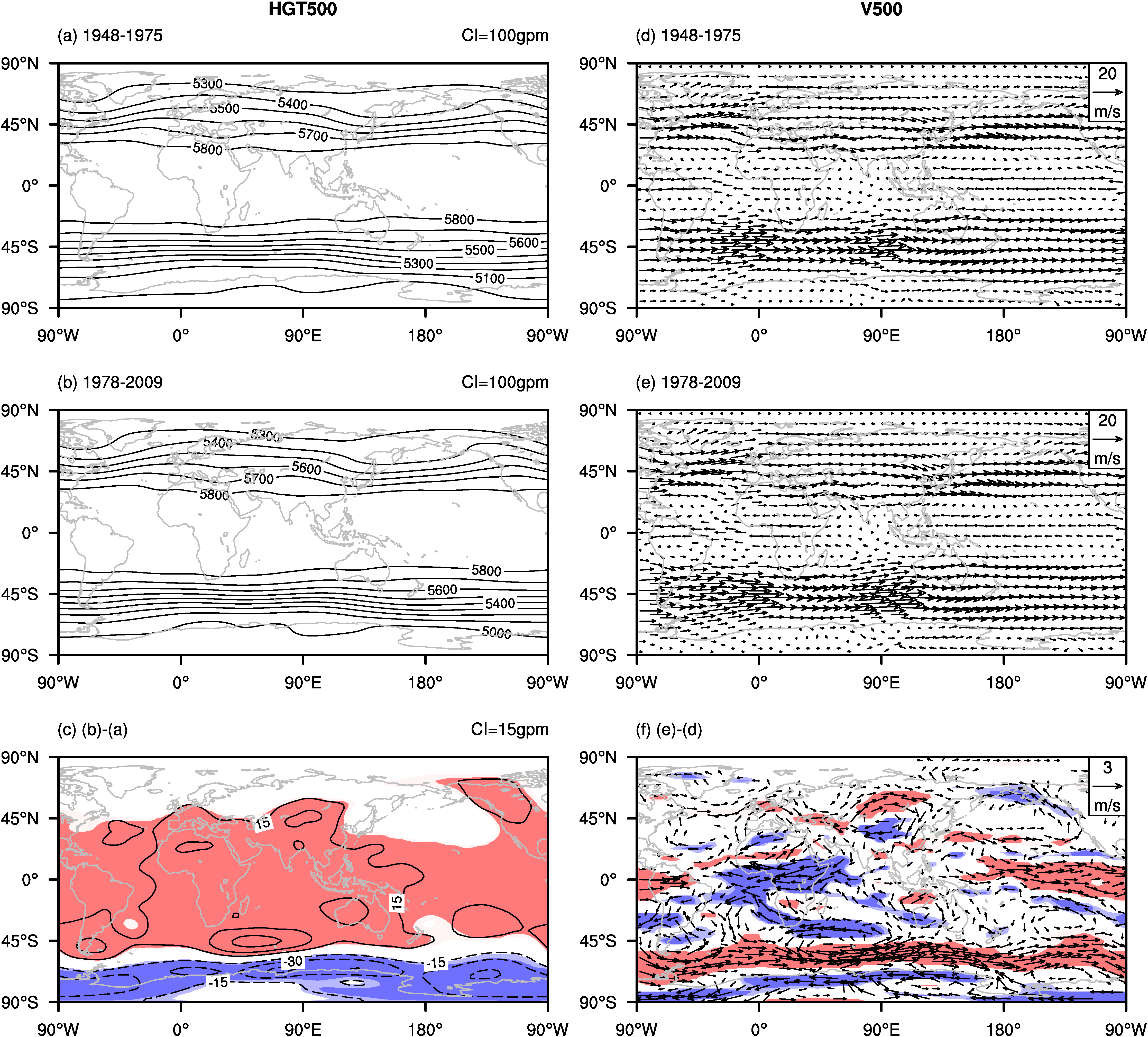
The annual mean geopotential height and winds show similar patterns during the periods 1948–1975 and 1978–2009 (Figure 2a,b,d,e), but their differences between the two sub-periods are distinct, and exceed the 95% confidence levels in many regions (Figure 2c,f). This suggests that the atmospheric basic flows were quite different before and after the mid-1970s. These changes in the basic flow may have had some impact on the characteristics of the ISO and QBWO. To reveal the possible effects of the atmospheric basic flow, the long-term means derived from 1948–1975 and 1978–2009 are used as the mean flow in Equations (1)–(3), respectively. This procedure will yield the spatial spectrum coefficients , , and for the sub-periods before and after the mid-1970s from Equation (7). Substituting these coefficients into Equation (8) yields the two ordinary differential equations
where subscripts a and b represent the periods 1948–1975 and 1978–2009, respectively. Equations (9) and (10) will be solved using the boundary conditions and method introduced above. Here, the symbols and are 396 × 396 matrixes, m, m, and m s−1. The eigenvalues of matrix and were further calculated with the following form:
where and are the growth rates of the perturbations before and after the mid-1970s. Positive and values indicate that the perturbations are unstable and can grow [51]. Their inverses (i.e., and ) are the e-folding times of perturbation growth. The shorter the e-folding time is, the easier and faster the perturbation grows. The values of and are the frequencies of the perturbations.
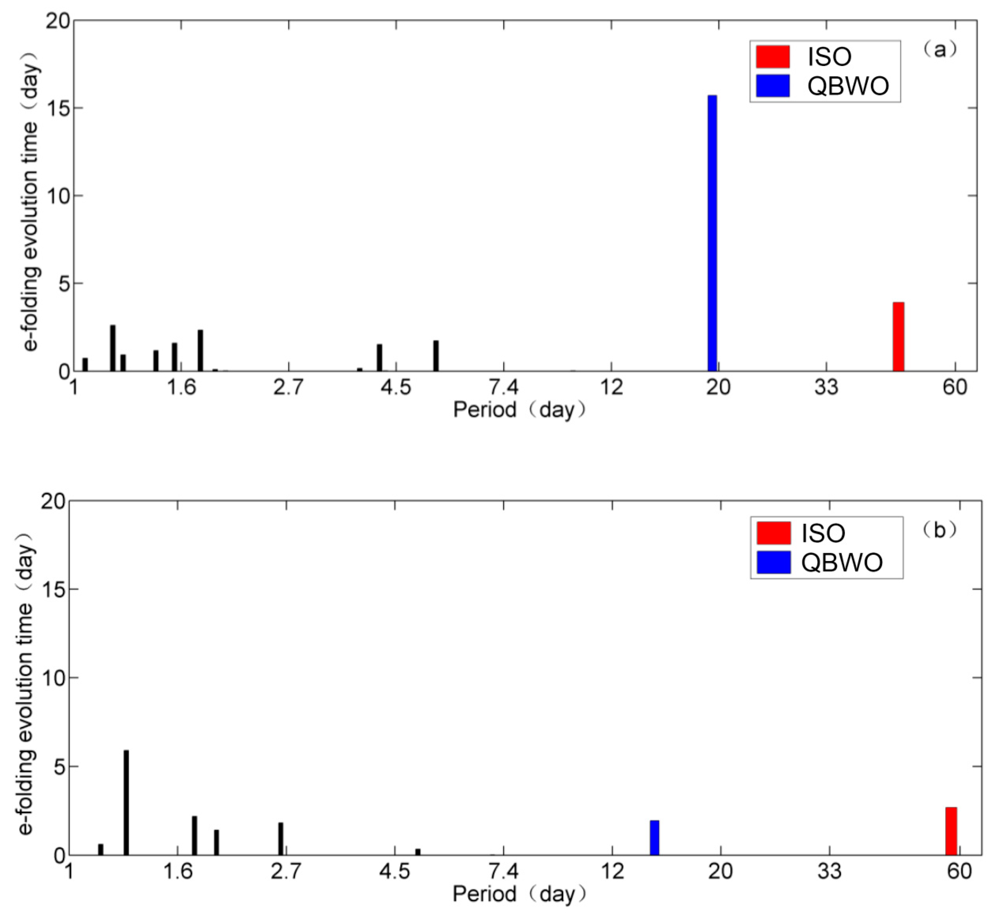
Figure 3 shows the e-folding time for disturbances with different periods during the periods 1948–1975 (Figure 3a) and 1978–2009 (Figure 3b). The least stable modes are mainly observed in three bands: the band below 10 days, the QBWO band, and the ISO band. Before the mid-1970s, the least stable mode of the QBWO had an e-folding time of approximately 15 days, and that of the ISO had an e-folding time of approximately four days (Figure 3a). After the mid-1970s, the e-folding time of the QBWO decreased to approximately two days, and that of the ISO decreased to approximately three days (Figure 3b). The reduction of the e-folding time of both the ISO and QBWO after the mid-1970s suggests that the ISO and QBWO tended to grow more easily, which would be how they intensified after the mid-1970s. Considering that only the atmospheric basic flow was changed to solve Equations (1)–(3) for the two sub-periods, it is reasonable to conclude that the shorter e-folding time, and thereby the intensification of both the ISO and QBWO after the mid-1970s, can be attributed to the altered atmospheric basic flow. Hence, the change of the atmospheric basic flow is an important mechanism to explain the interdecadal intensification of the QBWO and the ISO after the mid-1970s.
4. Summary and Discussion
It is well-known that the climate system experienced a significant interdecadal change in the mid-1970s, which can be observed in both the atmospheric mean state and the interannual variability [16,46,48]. In this study, it was found that the strength of the global low-frequency oscillation, including both the ISO and the QBWO, intensified significantly after the mid-1970s. The intensification of the ISO and QBWO can be observed from the lower to the upper troposphere with barotropic structure, so the linearized non-dimensional barotropic model is employed to investigate the involved mechanism of the observed change.
The spatial spectrum expansion method is capable of reconstructing the large-scale feature of the global geopotential height and horizontal wind fields, and it was used to solve the barotropic model. Considering the distinct changes of the atmospheric mean flow in the mid-1970s, the barotropic model was solved with two different atmospheric basic flows derived from the averages of 1948–1975 and 1978–2009, respectively. It reveals that the e-folding time of both the ISO and QBWO was shorter during 1978–2009 than during 1948–1975. This result suggests that the ISO and QBWO tend to grow more easily and intensify after the mid-1970s, consistent with the observed changes of the ISO and QBWO. Because nothing changes in the barotropic model except the atmospheric basic state, these results suggest that the observed intensification of the ISO and QBWO after the mid-1970s can be largely attributed to the altered atmospheric basic flow.
Previous studies suggest that atmospheric basic flow can influence the low-frequency oscillation in many ways. For example, Li et al. [44] found that a westerly profile is the most important factor for the least stable modes, and that the intensity and meridional gradient of the basic flow are of secondary importance. In this study, the role of atmospheric basic flow is emphasized in order to explain the observed interdecadal changes of the ISO and QBWO, but it remains unclear in our analyses which characteristics of the altered basic flow play the key roles. Besides, this study focuses on the global feature of the low-frequency oscillation, and cannot explain the regional changes, i.e., the spatial structure, of the ISO and QBWO. These remaining issues will be investigated with a more complicated model in our following studies. Last but not least, a second interdecadal shift was observed in many regions of the world in the late 1990s and early 2000s [52,53,54,55,56,57,58], after the well-documented climate shift in the mid-1970s, and it would be interesting to investigate whether the strength of the ISO and QBWO experience some changes accordingly. However, fewer than 20 years have passed since the climate shift of the late 1990s or early 2000s, and this relatively short period may not yield a stationary basic state to perform analyses like those in this study. Therefore, this issue will remain open currently and will be investigated in the future.
Author Contributions
R.Y. and Q.C. designed the research, R.Y. and Y.L. performed the analyses, R.Y., Q.C. and L.W. interpreted the results and wrote the paper.
Funding
This study was supported by the National Natural Science Foundation of China (Grant No. 41721004, U1502233) and the Chinese Academy of Sciences (Grant No. QYZDY-SSW-DQC024).
Acknowledgments
We thank the two anonymous reviewers for their insightful suggestions that helped to improve the manuscript.
Conflicts of Interest
The authors declare there is no conflicts of interest regarding the publication of this paper.
References
- Mao, J.Y.; Sun, Z.; Wu, G.X. 20–50-day oscillation of summer Yangtze rainfall in response to intraseasonal variations in the subtropical high over the western North Pacific and South China Sea. Clim. Dyn. 2010, 34, 747–761. [Google Scholar] [CrossRef]
- He, J.H.; Lin, H.; Wu, Z.W. Another look at influences of the Madden-Julian Oscillation on the wintertime East Asian weather. J. Geophys. Res. Atmos. 2011, 116. [Google Scholar] [CrossRef] [Green Version]
- Lu, R.Y.; Dong, H.L.; Su, Q.; Ding, H. The 30–60-day intraseasonal oscillations over the subtropical western North Pacific during the summer of 1998. Adv. Atmos. Sci. 2014, 31, 1–7. [Google Scholar] [CrossRef]
- Madden, R.A.; Julian, P.R. Description of Global-Scale Circulation Cells in the Tropics with a 40–50 Day Period. J. Atmos. Sci. 1972, 29, 1109–1123. [Google Scholar] [CrossRef]
- Madden, R.A.; Julian, P.R. Detection of a 40–50 Day Oscillation in the Zonal Wind in the Tropical Pacific. J. Atmos. Sci. 1971, 28, 702–708. [Google Scholar] [CrossRef] [Green Version]
- Murakami, M. Analysis of Summer Monsoon Fluctuations over India. J. Meteorol. Soc. Jpn. 1976, 54, 15–31. [Google Scholar] [CrossRef] [Green Version]
- Krishnamurti, T.N.; Bhalme, H.N. Oscillations of a Monsoon System. Part I. Observational Aspects. J. Atmos. Sci. 1976, 33, 1937–1954. [Google Scholar] [CrossRef] [Green Version]
- Ghil, M.; Mo, K. Intraseasonal Oscillations in the Global Atmosphere. Part I: Northern Hemisphere and Tropics. J. Atmos. Sci. 1991, 48, 752–779. [Google Scholar] [CrossRef] [Green Version]
- Madden, R.A.; Julian, P.R. Observations of the 40–50-day tropical oscillation—A review. Mon. Weather Rev. 1994, 122, 814–837. [Google Scholar] [CrossRef]
- Goswami, B.N.; Mohan, R.S.A. Intraseasonal oscillations and interannual variability of the Indian summer monsoon. J. Clim. 2001, 14, 1180–1198. [Google Scholar] [CrossRef]
- Foltz, G.R.; McPhaden, M.J. The 30–70 day oscillations in the tropical Atlantic. Geophys. Res. Lett. 2004, 31, 1–4. [Google Scholar] [CrossRef]
- Wang, B.; Webster, P.; Kikuchi, K.; Yasunari, T.; Qi, Y. Boreal summer quasi-monthly oscillation in the global tropics. Clim. Dyn. 2006, 27, 661–675. [Google Scholar] [CrossRef]
- Wen, M.; Li, T.; Zhang, R.; Qi, Y.J. Structure and Origin of the Quasi-Biweekly Oscillation over the Tropical Indian Ocean in Boreal Spring. J. Atmos. Sci. 2010, 67, 1965–1982. [Google Scholar] [CrossRef]
- Wen, M.; Zhang, R.H. Quasi-Biweekly Oscillation of the Convection around Sumatra and Low-Level Tropical Circulation in Boreal Spring. Mon. Weather Rev. 2008, 136, 189–205. [Google Scholar] [CrossRef]
- Sobel, A.H.; Maloney, E.D.; Bellon, G.; Frierson, D.M. The role of surface heat fluxes in tropical intraseasonal oscillations. Nat. Geosci. 2008, 1, 653–657. [Google Scholar] [CrossRef]
- Cao, J.; Wen, Z.P.; Chang, Y.L.; Li, X.R. Wavelet analysis of the convectively-coupled equatorial waves. Sci. China Earth Sci. 2012, 55, 675–684. [Google Scholar] [CrossRef]
- Wang, L.; Kodera, K.; Chen, W. Observed triggering of tropical convection by a cold surge: Implications for MJO initiation. Q. J. R. Meteorol. Soc. 2012, 138, 1740–1750. [Google Scholar] [CrossRef]
- Zhang, C.D. Madden-Julian oscillation. Rev. Geophys. 2005, 43, 1–36. [Google Scholar] [CrossRef]
- Li, T.; Wang, B. A review on the western north pacific monsoon: Synoptic-to-interannualvariabilities. Terr. Atmos. Ocean. Sci. 2005, 16, 285–314. [Google Scholar] [CrossRef]
- Ha, K.J.; Heo, K.Y.; Lee, S.S.; Yun, K.S.; Jhun, J.G. Variability in the East Asian monsoon: A review. Meteorol. Appl. 2012, 19, 200–215. [Google Scholar] [CrossRef]
- Lee, J.Y.; Fu, X.H.; Wang, B. Predictability and prediction of the Madden-Julian Oscillation: A review on progress and current status. In The Global Monsoon System: Research and Forecast, 3rd ed.; World Scientific: Singapore, 2017; pp. 147–159. [Google Scholar]
- Wheeler, M.C.; Kim, H.J.; Lee, J.Y.; Gottschalck, J.C. Real-time forecasting of modes of tropical intraseasonal variability: The Madden-Julian and boreal summer intraseasonal oscillations. In The Global Monsoon System: Research and Forecast, 3rd ed.; World Scientific: Singapore, 2017; pp. 131–138. [Google Scholar]
- Li, C.Y. Actions of summer monsoon troughs (ridges) and tropical cyclone over South Asia and moving CISK mode. Sci. Sin. Ser. B 1985, 28, 1197–1206. [Google Scholar] [CrossRef]
- Lau, K.M.; Peng, L. Origin of Low-Frequency (Intraseasonal) Oscillations in the Tropical Atmosphere. Part I: Basic Theory. J. Atmos. Sci. 1987, 44, 950–972. [Google Scholar] [CrossRef] [Green Version]
- Takahashi, M. A Theory of the Slow Phase Speed of the Intraseasonal Oscillation using the Wave-CISK. J. Meteorol. Soc. Jpn. Ser. II 1987, 65, 43–49. [Google Scholar] [CrossRef] [Green Version]
- Chang, C.P.; Lim, H. Kelvin wave-CISK: A possible mechanism for the 30–50 day oscillations. J. Atmos. Sci. 1988, 45, 1709–1720. [Google Scholar] [CrossRef]
- Li, C.Y. Dynamical study on 30–50 day oscillation in the tropical atmosphere outside Equator. Chin. J. Atmos. Sci. 1990, 14, 83–92. (In Chinese) [Google Scholar] [CrossRef]
- Emanuel, K.A. An Air-Sea Interaction Model of Intraseasonal Oscillations in the Tropics. J. Atmos. Sci. 1987, 44, 2324–2340. [Google Scholar] [CrossRef] [Green Version]
- Neelin, J.D.; Held, I.M.; Cook, K.H. Evaporation-Wind Feedback and Low-Frequency Variability in the Tropical Atmosphere. J. Atmos. Sci. 1987, 44, 2341–2348. [Google Scholar] [CrossRef] [Green Version]
- Li, C.Y.; Xiao, Z.N. The 30–60 day oscillations in the global atmosphere excited by warming in the equatorial eastern Pacific. Chin. Sci. Bull. 1992, 37, 484–489. [Google Scholar]
- Li, W.B.; Ji, L.R. Mechanisms of the atmospheric Teleconnection Associated with the Activity of the Asian Summer Monsoon Part II: Optimal Forcing and Atmospheric Responses. Chin. J. Atmos. Sci. 1999, 23, 571–580. (In Chinese) [Google Scholar] [CrossRef]
- Li, W.B.; Ji, L.R. Mechanisms of the atmospheric teleconnection associated with activity of the Asian summer monsoon part I: Analyses of the normal modes and the finite Time unstable singular vectors. Chin. J. Atmos. Sci. 1999, 23, 477–486. (In Chinese) [Google Scholar] [CrossRef]
- Li, C.Y.; Liao, H.Q. Behaviour of coupled modes in a simple nonlinear air-sea interaction model. Adv. Atmos. Sci. 1996, 13, 183–195. [Google Scholar] [CrossRef]
- Wang, B.; Xie, X.S. Coupled modes of the warm pool climate system. Part I: The role of air-sea interaction in maintaining Madden-Julian oscillation. J. Clim. 1998, 11, 2116–2135. [Google Scholar] [CrossRef]
- Goswami, P.; Mathew, V. A Mechanism of Scale Selection in Tropical Circulation at Observed Intraseasonal Frequencies. J. Atmos. Sci. 1994, 51, 3155–3166. [Google Scholar] [CrossRef] [Green Version]
- Chatterjee, P.; Goswami, B.N. Structure, genesis and scale selection of the tropical quasi-biweekly mode. Q. J. R. Meteorol. Soc. 2004, 130, 1171–1194. [Google Scholar] [CrossRef] [Green Version]
- Frederiksen, J.S.; Frederiksen, C.S. Monsoon disturbances, intraseasonal oscillations, teleconnection patterns, blocking, and storm tracks of the global atmosphere during January 1979: Linear theory. J. Atmos. Sci. 1993, 50, 1349–1372. [Google Scholar] [CrossRef]
- Frederiksen, J.S. A Unified Three-Dimensional Instability Theory of the Onset of Blocking and Cyclogenesis. II. Teleconnection Patterns. J. Atmos. Sci. 1983, 40, 2593–2609. [Google Scholar] [CrossRef] [Green Version]
- Frederiksen, J.S. A Unified Three-Dimensional Instability Theory of the Onset of Blocking and Cyclogenesis. J. Atmos. Sci. 1982, 39, 969–982. [Google Scholar] [CrossRef]
- Simmons, A.J.; Wallace, J.M.; Branstator, G.W. Barotropic Wave Propagation and Instability, and Atmospheric Teleconnection Patterns. J. Atmos. Sci. 1983, 40, 1363–1392. [Google Scholar] [CrossRef] [Green Version]
- Yang, D.S.; Cao, W.Z. A Possible Dynamic Mechanism of the Atmospheric 30–60 Day Period Oscillation in the Extratropical Latitude. Chin. J. Atmos. Sci. 1995, 19, 209–218. (In Chinese) [Google Scholar] [CrossRef]
- Li, C.Y.; Wu, P.L.; Zhang, Q. Some characters of the 30–60 day oscillation in the atmospheric circulation in North Hemisphere. Sci. China Ser. B Chem. Life Sci. Earth Sci. 1990, 20, 764–774. (In Chinese) [Google Scholar] [CrossRef]
- Li, C.Y.; Zhang, Q. Global atmospheric low-frequency teleconnection. Prog. Nat. Sci. Int. 1991, 1, 447–452. [Google Scholar]
- Li, C.Y.; Cao, W.Z.; Li, G.L. Effect of basic flow on triggering the instability of atmospheric intraseasonal oscillation in mid-high latitudes. Sci. China Ser. B Chem. Life Sci. Earth Sci. 1995, 25, 978–985. (In Chinese) [Google Scholar] [CrossRef]
- Chen, T.C.; Chen, J.M. The 10–20-Day Mode of the 1979 Indian Monsoon: Its Relation with the Time Variation of Monsoon Rainfall. Mon. Weather Rev. 1993, 121, 2465–2482. [Google Scholar] [CrossRef] [Green Version]
- Trenberth, K.E.; Hurrell, J.W. Decadal atmosphere-ocean variations in the Pacific. Clim. Dyn. 1994, 9, 303–319. [Google Scholar] [CrossRef]
- Wang, L.; Chen, W.; Huang, R.H. Changes in the variability of north pacific oscillation around 1975/1976 and its relationship with East Asian winter climate. J. Geophys. Res. 2007, 112, 1–13. [Google Scholar] [CrossRef]
- Liu, Y.Y.; Yu, Y.Q.; He, J.H.; Zhang, Z.G. Characteristics and numerical simulation of the tropical intraseasonal oscillations under global warming. Acta Meteorol. Sin. 2006, 64, 723–733. [Google Scholar]
- Kalnay, E.; Kanamitsu, M.; Kistler, R.; Collins, W.; Deaven, D.; Gandin, L.; Iredell, M.; Saha, S.; White, G.; Woollen, J.; et al. The NCEP/NCAR 40-year reanalysis project. Bull. Am. Meteorol. Soc. 1996, 77, 437–471. [Google Scholar] [CrossRef]
- Cao, J.; You, Y.L. New method for low order spectral model and its application. Appl. Math. Mech. 2006, 27, 477–484. [Google Scholar] [CrossRef]
- Li, C.Y. Excitation of the atmospheric unstable modes (chapter 4.3). In An Introduction to Climate Dynamics, 2nd ed.; China Meteorological Press: Beijing, China, 2000; pp. 136–149. (In Chinese) [Google Scholar]
- Wang, L.; Xu, P.Q.; Chen, W.; Liu, Y. Interdecadal variations of the Silk Road pattern. J. Clim. 2017, 30, 9915–9932. [Google Scholar] [CrossRef]
- Wang, L.; Chen, W. The East Asian winter monsoon: Re-amplification in the mid-2000s. Chin. Sci. Bull. 2014, 59, 430–436. [Google Scholar] [CrossRef]
- Byshev, V.I.; Neiman, V.G.; Anisimov, M.V.; Gusev, A.V.; Serykh, I.V.; Sidorova, A.N.; Figurkin, A.L.; Anisimov, I.M. Multi-decadal oscillations of the ocean active upper-layer heat content. Pure Appl. Geophys. 2017, 174, 2863–2878. [Google Scholar] [CrossRef]
- Ponomarev, V.I.; Dmitrieva, E.V.; Shkorba, S.P.; Karnaukhov, A.A. Change of the global climate region at the turn of the XX–XXI centuries. Vestnik MGTU 2018, 21, 160–169. [Google Scholar] [CrossRef]
- Zhang, J.Y.; Wang, L.; Yang, S.; Chen, W.; Huangfu, J.L. Decadal changes of the wintertime tropical tropospheric temperature and their influences on the extratropical climate. Chin. Sci. Bull. 2016, 61, 737–744. [Google Scholar] [CrossRef]
- Gu, W.; Wang, L.; Hu, Z.Z.; Hu, K.M.; Li, Y. Interannual variations of the first rainy season precipitation over south China. J. Clim. 2017, 31, 623–640. [Google Scholar] [CrossRef]
- Zhang, R.H. Changes in East Asian summer monsoon and summer rainfall over eastern China during recent decades. Chin. Sci. Bull. 2015, 60, 1222–1224. [Google Scholar] [CrossRef]
Figure 1.
The ratio of global grid numbers whose geopotential height exceeds the 95% confidence level for different temporal bands at the (a) 850 hPa level; (b) 500 hPa level; and (c) 200 hPa level, respectively. The averaged spectrum values for the two sub-periods 1948–1975 and 1978–2009 at the (d) 850 hPa level; (e) 500 hPa level; and (f) 200 hPa level, respectively. The black solid lines in (a–c) and red solid lines in (d–f) denote the intra seasonal oscillation (ISO) band. The red dotted lines in (a–f) denote the quasi-biweekly oscillation (QBWO) band.
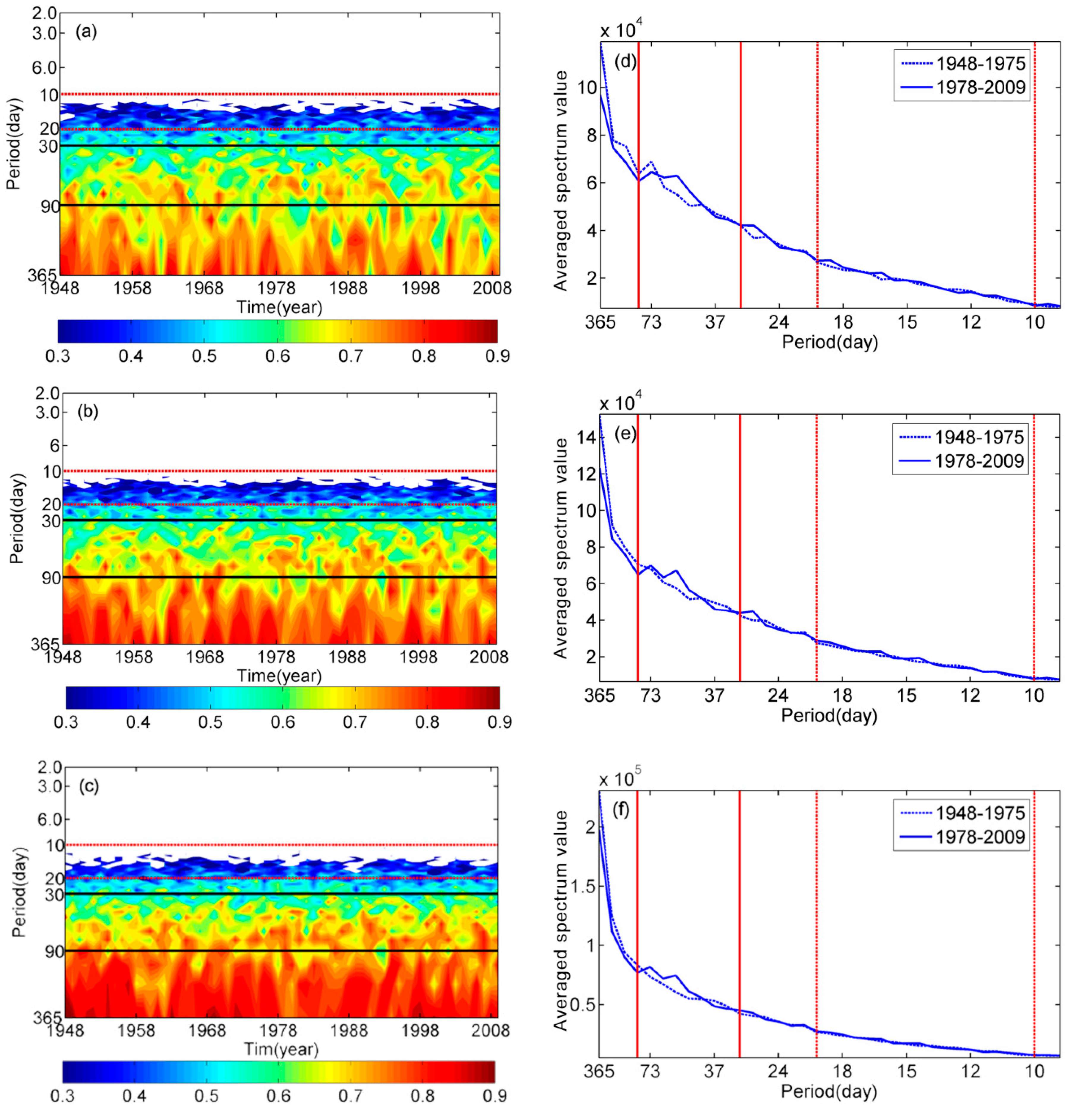
Figure 2.
The annual mean 500 hPa geopotential height during the sub-periods (a) 1948–1975; (b) 1978–2009; and (c) their difference (i.e., (b) minus (a)); (d–f) are the same as (a–c), but for the annual mean 500 hPa winds. Negative values are dashed, and zero contours are omitted in (c). Dark and light shading indicates 99% and 95% confidence levels based on two-tailed Student’s t-test, respectively. Zonal winds are used to evaluate the confidence level in (f).

Figure 3.
The e-folding time for perturbations of different temporal bands during the periods (a) 1948–1975 and (b) 1978–2009. The red and blue bars indicate the ISO and QBWO bands, respectively.
Figure 3.
The e-folding time for perturbations of different temporal bands during the periods (a) 1948–1975 and (b) 1978–2009. The red and blue bars indicate the ISO and QBWO bands, respectively.


Table 1.
The averaged spectrum values and their differences in the ISO and QBWO bands for the two sub-periods before and after the mid-1970s.
Table 1.
The averaged spectrum values and their differences in the ISO and QBWO bands for the two sub-periods before and after the mid-1970s.
| ISO | QBWO | |||||
|---|---|---|---|---|---|---|
| 850 hPa | 500 hPa | 200 hPa | 850 hPa | 500 hPa | 200 hPa | |
| 1948–1975 | 59,193 | 61,710 | 67,835 | 23,294 | 24,181 | 22,865 |
| 1978–2009 | 61,348 | 64,397 | 73,209 | 24,438 | 25,318 | 23,616 |
| confidence level of difference | 90% | 96% | 99.6% | 92% | 93% | 83% |
© 2018 by the authors. Licensee MDPI, Basel, Switzerland. This article is an open access article distributed under the terms and conditions of the Creative Commons Attribution (CC BY) license (http://creativecommons.org/licenses/by/4.0/).
Share and Cite
MDPI and ACS Style
Yang, R.; Chen, Q.; Liu, Y.; Wang, L. A Mechanism of the Interdecadal Changes of the Global Low-Frequency Oscillation. Atmosphere 2018, 9, 292. https://doi.org/10.3390/atmos9080292
AMA Style
Yang R, Chen Q, Liu Y, Wang L. A Mechanism of the Interdecadal Changes of the Global Low-Frequency Oscillation. Atmosphere. 2018; 9(8):292. https://doi.org/10.3390/atmos9080292
Chicago/Turabian StyleYang, Ruowen, Quanliang Chen, Yuyun Liu, and Lin Wang. 2018. "A Mechanism of the Interdecadal Changes of the Global Low-Frequency Oscillation" Atmosphere 9, no. 8: 292. https://doi.org/10.3390/atmos9080292
Note that from the first issue of 2016, this journal uses article numbers instead of page numbers. See further details here.