A Nowcasting Model for Tropical Cyclone Precipitation Regions Based on the TREC Motion Vector Retrieval with a Semi-Lagrangian Scheme for Doppler Weather Radar

Abstract

Accurate observational data and reliable prediction models are both essential to improve the quality of precipitation forecasts. The spiraling trajectories of air parcels within a tropical cyclone (TC) coupled with the large sizes of these systems brings special challenges in making accurate short-term forecasts, or nowcasts. Doppler weather radars are ideal instruments to observe TCs when they move over land, and traditional nowcasts incorporate radar data. However, data from dozens of radars must be mosaicked together to observe the entire system. Traditional single-radar-based reflectivity tracking methods commonly employed in nowcasting are not suitable for TCs as they are not able to capture the circular motion of these systems. Thus, this paper focuses on improving short-term predictability of TC precipitation with Doppler weather radar observations based on: a multi-scale motion vector retrieval algorithm, an optimization technique and a semi-Lagrangian advection scheme. Motion fields of precipitation regions are obtained by a multi-level motion vector retrieval algorithm, then corrected and smoothed by the optimization technique using mass and smooth constraints. Predicted precipitation regions are then extrapolated using the semi-Lagrangian advection scheme. A case study of Hurricane Isabel (2003) shows that the combination of these methods may increase reliable rainfall prediction to about 5 h as the TC moves over land.

1. Overview

1.1. Tropical Cyclone and Precipitation Nowcasting

As tropical cyclones (TCs) approach land, they pose a danger to life and property with their associated fast winds, storm surges and rainfall. Once they move inland, many of the forecasting challenges and death stem from heavy rainfall [1,2]. An accurate short-term forecast of 0–6 h of precipitation from tropical cyclones (TCs) is required by forecasters and decision makers for the issuance of flash flood warnings and urban drainage management [3]. This kind of short-time forecasting is called “nowcasting”. The World Meteorological Organization (WMO) defines nowcasting as “the detailed description of the current weather along with forecasts obtained by extrapolation for a period of 0–6 h ahead” [4]. Nowcasting incorporates the most recent observations, including those from radars and satellites, to make an accurate forecast for small regions such as cities. A successful nowcast that gives an accurate rainfall prediction will significantly reduce the hazardous risk to people and properties if flood-prone areas can be avoided [5].

In the United States, the Weather Surveillance Radar-1988 Doppler (WSR-88D), or Next Generation Weather Radar (NEXRAD), a network of S-band radars, has been operational since 1995. Approximately 160 radars provides non-stop high-resolution weather observation data for precipitating regions and their trajectories at 0.25–1 km, every 5–10 min [6,7]. Thus, the weather radar network is an important data source in weather forecasting, including nowcasting. In general, radar data can be used in nowcasting in two different ways: predicting only based on weather radar data (radar-only nowcasting), or predicting using a numeric weather prediction (NWP) model with radar observations digested by data-assimilation procedure. Radar-only nowcasting is usually based on object tracking and extrapolation methods in image processing technologies. It analyzes a time series of radar products, usually reflectivity data, plotted as digital images, and identifies and extracts the tracks of coherent cloud structures from one image to the next. Then, extrapolation is done by moving pixels on the last image following the extracted track from the image series. Because using image processing techniques ignores physical rules in the atmosphere, radar-only nowcasting cannot produce a reliable prediction for days into the future in NWP models. In contrast, radar-assimilated model nowcasting does not suffer from this problem because it uses physical (deterministic) equations to solve clouds’ thermodynamic processes to predict their future status, and that prediction is expected to be more reliable [8]. For example, the recently-developed RAPid refresh model (RAP) digests weather radar observations through a data-assimilation system, and it can produce a fast prediction up to 18 h into the future nationwide with updates every 60 min [9]. Although theoretically, using an NWP model that assimilates radar observations to issue forecasts should surpass using radar observations only, it cannot replace radar-based nowcasting yet. Firstly, using numeric weather models in nowcasting is heavily limited by the quality of observational data. Since NWP models are sensitive to initial conditions, setting up accurate initial conditions is critical in short-term forecasting. Thus, additional quality control procedures are required for radar-data assimilation besides normal radar data quality control techniques (e.g., removing ground clutters, non-meteorological echoes, sun strobes) [10], while those high-quality data may not be available in an emergent situation [3]. Secondly, radar-only nowcasting requires significantly less computational resources than NWP models. Modern NWP models require thousands of CPUs to reach a spatial resolution of 1 km on a nationwide domain, and 1 km is also a resolution limit for many NWP models due to computing resources and/or the timeliness of the forecast. In contrast, data from current operational WSR-88D radars can be obtained at a spatial resolution up to 250 m, and extrapolating radar observations requires less than one hundred CPUs with this finer resolution [11]. Finally, radar reflectivity is not an explicit measurement of liquids in the atmosphere; rather, it is an aggregated reading contributed by both the total solid or liquid volume of hydrometeor drop size. Because hydrometeor drop size contributes exponentially to the reflectivity echo strength, a few large drops can produce the same reflectivity reading as many small rain drops, whose actual total liquid volume is smaller than the later. When an NWP model must assume a drop size distribution to calculate “simulated reflectivity” [12] before comparison with observed reflectivity, such drop size distributions are sampled from field experiments under non-extreme conditions [13]. This means that the “simulated reflectivity” may not produce results equivalent to radar-observed reflectivity, especially in convective and extreme weather scenarios, including TCs [14]. Thus, although the concepts and theories in the NWP models are more advanced than extrapolation-based methods, radar-only nowcasting is still applied operationally in many countries and cannot be replaced by NWP models.

1.2. State-of-the-Art Radar-Based Nowcasting Methods

Traditional radar-only-based (radar-based hereafter) nowcasting is mostly based on observations from a single radar. Tracking radar echo by correlation (TREC) is the first kind of radar-based nowcasting method, proposed by [15]. It calculates correlation coefficients between successive images of radar echoes and uses the maximum values to obtain the motion vectors of different regions. TREC is an image processing algorithm that is purely-based on image sequences and completely ignores scale and dynamical equations of motion for a weather system. To overcome these drawbacks and improve accuracy, multiple refined methods have been proposed after TREC. The work in [16] added a spatial filter to obtain the internal motion at a smaller scale. The work in [17] proposed the continuity of TREC vectors (COTREC) scheme to comply with the continuity constraint in the atmosphere. This constraint helped avoid the strong divergence of echoes that occurs in TREC results, but during calculations, it unavoidably weakened the retrieved wind field at the same time. The work in [18] showed that average echo motion speed obtained using COTREC was underestimated by 10% compared with the speed detected by an aircraft. The work in [19] was the first study to introduce a parameter in both the TREC and COTREC schemes to take into consideration the growth and decay of individual cloud regions. Its demonstration through analyses of local thunderstorm cases showed that the inclusion of a growth parameter led to a better forecast. The work in [20] combined COTREC and a shape analysis approach to track precipitation events and obtained a more refined motion vector field that reached a 70% match with ground observations, which was a better performance when compared to using COTREC only (40–50% matching). Besides the limitation on continuity, TREC occasionally produces a vector that points to a direction that is contradictory when compared with its surrounding vectors. This limitation was addressed by [21], who proposed the difference image-based TREC (DITREC) algorithm by calculating the cross-correlation maximum between differences in precipitating regions from three consecutive images instead of two images. The work in [8] introduced a blending algorithm that combines TREC vectors with model-predicted winds to prolong the prediction time up to 3 h. The work in [22] proposed the multi-scale TREC (MTREC) algorithm that uses TREC in a nested style: a first pass of TREC calculation with low resolution obtains the synoptic-scale motion, and one additional pass at high resolution inside each large low-resolution region is used to predict meso- to local-scale internal motion. They reported that MTREC could produce a reliable 3-h forecast in typhoon cases with input mosaics of composite reflectivity.

Operationally, TREC and all TREC-derived nowcasting methods are still based on single-radar scenarios. In the U.S., a single WSR-88D radar station can only cover a circular region with a 230-km radius when measuring the radial winds.Thus, using observations from a single radar station puts an upper limit on the spatial scale of observations and, consequently, also on the timescale over which the forecast is useful. The total time length of useful forecasts reported in the literature is usually less than 2 h and often less than 1 h [19]. Extending these methods to adopt a large mosaic of radar images obtained from multiple stations in a network permits forecasters to reveal cloud patterns that are not observable in single radar scenarios. For example, in a single-radar range, non-linear motions like rotation in a mesoscale convective system may not be significant due to their limited spatio-temporal scale, but such rotation can be easily captured in a large domain [16]. Furthermore, it is suggested by previous research [23] that patterns at about a 1000-km scale tend to be more consistent and predictable up to one day. Thus, it is more preferable to perform nowcasting at a synoptic scale when data are available from multiple radar stations and can be mosaicked into a single image.

1.3. Motivation and Goals

We find that research applying TREC and TREC-derived methods mainly reports their predictability on local heavy and extreme rainfall cases like convective storms, localized thunderstorms and squall lines that are captured well by a single radar. We only found a single MTREC case-study that featured a partial view of a small typhoon before landfall using a single radar station. A few researchers have employed TREC to retrieve winds in landfalling TCs. The authors in [18] performed their analysis on a Cartesian coordinate system and determined that performance was best when vertical wind shear was weak. Tropical cyclone cases should be treated separately from other weather systems because TCs are predominately large and have a strong rotational component to their motion. The linear extrapolation methods used by most TREC-derived algorithms ignore the tangential component of motion. Therefore, the predicted motion vectors would break the storm apart. To better account for the tangential component of a TC’s motion, the work in [24] employed a polar grid centered over the circulation center and arc-shaped search areas and correlation cells. The work in [25] developed T -TREC specifically to analyze the winds of TCs and in addition to analysis on the polar grid, included an objective algorithm to determine the TC center and estimate the search radius. This improved representation of the TC’s core reduced bias from 5 m/s reported by Tuttle and Gall to less than 4 m/s. Subsequent research by [26,27,28] used wind fields derived from the T-TREC method for data assimilation and demonstrated improved TC precipitation forecasts.

Although convective clouds with relatively strong vertical motion and small horizontal extent occur in the eye wall and spiral rain bands of TCs, most of the clouds that comprise a TC are stratiform [29], where vertical motion is relatively weak and the clouds occupy a large horizontal region. The previous studies employing TREC or its derivatives mostly focused on either convective or stratiform cases, not the mixed scenario that occurs with a TC. Furthermore, although the average extent of a TC’s rainfall is 220–240 km on either side of its circulation center [30,31], it is generally considered that rainfall within a 500-km radius from a TC’s eye is produced by the TC rather than another type of weather system [32]. This 500-km distance obviously exceeds the detection range of one radar station. As such rainfall can potentially trigger flooding [33], it is critical to accurately predict its motion, but the scale of a TC’s rain bands necessitates that multiple radars be employed to capture the entire system.

Given the radar network’s ability to observe the atmosphere at a horizontal resolution of 0.5–1 km and temporal resolution of about 5 min, it is a powerful instrument to study and forecast TCs before, during and after their landfall. Thus, in this study, we aim to extend the capability of the original single-radar nowcasting method to a large domain and tune the algorithm to consider tangential motion and mixed cloud types for a TC scenario. We choose TREC as our starting point, then employ multiple ideas from related methods to adopt it for a TC scenario. It is noticeable that in this study, we exclusively derive cloud motions by analyzing a sequence of radar images, rather than utilizing radial Doppler velocity moments. Wind velocity retrieved from Doppler velocity is not equal to the velocity of cloud motions, and in precipitation areas, the effect of wind velocity is often overridden by cloud dynamics, which produce the precipitation (e.g., an embed cell in a spiral band of a TC may show a different direction of wind velocity at its location). For the same reason, in this paper, we use term “motion vectors” instead of “velocity” to describe computed cloud movements. The rest of the paper is arranged as follows. Section 2 presents our revised nowcasting scheme for a multi-radar scenario with special considerations when a TC is observed. To provide a performance evaluation, Section 3 presents a 10-h nowcast of the precipitation associated with Hurricane Isabel as it moved over the mid-Atlantic and northeastern U.S. in September of 2003. The last section concludes this study and presents directions for future research.

2. Methodology

2.1. Overview

As a prediction model, a nowcasting model shares the same features as any general prediction model: it takes observed data as inputs and generates outputs beyond the observed time period. As radar-only-based nowcasting lacks many fundamental physical variables to establish a numerical weather prediction, a general assumption is to treat all clouds in the atmosphere as ideal air parcels and use a trajectory or dispersion model. In this study, we divide our model into two stages: the tracking stage and forecast stage. In the tracking stage, trajectories are determined for each cloud. The tracking method is based on two modified methods: a modified MTREC and a smoothing step via an optimization technique based on [34]. For MTREC, we use its nested region-tracking scheme; for the optimization technique, we use a similar mathematical method like in a variational analysis. The forecasting stage starts immediately after the end of the tracking stage. In the forecast stage, the identified regions are extrapolated using a semi-Lagrangian trajectory model. For convenience, reflectivity values taken from weather radars are re-projected into a stack of raster layers at different altitudes with equally-sized square cells using the method described in [35]. These raster layers can be treated as digital images, and each cell containing a reflectivity value is represented as a pixel on an image; thus, we call them reflectivity images. Clouds and rainfall regions are both represented using pixels on these reflectivity images. In this study, a rainfall region is defined as those clustered pixels on the reflectivity images where cell values are larger than 10 dB Z. Although it is ideal to create a model to track movements for individual storms, as previously mentioned, TCs are mainly composed of stratiform clouds, and individual storm tracking techniques underperform in this scenario because cloud boundaries of individual storms are difficult to distinguish [36]. For example, if we define storm boundaries using a certain reflectivity threshold, two large regions of that reflectivity value may be connected by a single pixel to produce a single larger region, whereas the desired outcome would be to split the regions at the location of the single pixel. Thus, we decide to fallback to pixel-based nowcasting methods, which are utilized in all TREC-derived methods. The method produces a trajectory for each pixel.

2.2. Basic Method

The basic form of our nowcasting can be written as the following mathematic expressions:

$$\widehat{Z}(t_0+\tau ,\mathbf{x})=Z(t_0,\mathbf{x}-\alpha )-\tau Q(t_0,\mathbf{x}-\alpha )$$

(1)

It uses displacement vectors $\alpha$ and observation Z to predict $\widehat{Z}$ with a leading time of $\tau$. Changes of the rainfall rate are accounted for using a source/sink term Q.

Figure 1 and Figure 2 show the setup and general workflow of the tracking and predicting stages in this study. In the tracking stage, three motion fields are calculated from four consecutive images: t and $t+10$ min, $t+10$ min and $t+20$ min, $t+20$ min and $t+30$ min. Then, one motion field is set to the mean value of the three fields. This step adopts the DITREC idea of using the last several consecutive images to avoid disordered vectors. Then, in the next stage, the averaged motion is corrected using an optimization technique. During the prediction stage, a pixel’s displacement vector $\alpha$ is determined using a semi-Lagrangian extrapolation scheme [37] over the motion field domain. It is noticeable that a pixel’s displacement vector $\alpha$ is always from its start point $\mathbf{x}-\alpha$ to its end point $\mathbf{x}$, but its actual track may be a curve because it follows the cyclonic rotation in a TC. Details of these steps are explained in the following sections.

2.3. Calculating Motion Field

The basic method to obtain the displacement vector of a block is TREC. The first step is to calculate the correlation of two radar reflectivity images as:

$$R=\frac{\sum Z_1\left({\mathbf{x}}_1\right)Z_2\left({\mathbf{x}}_2\right)-\frac{\sum Z_1\left({\mathbf{x}}_1\right)\sum Z_2\left({\mathbf{x}}_2\right)}{n}}{\sqrt{(Z_1^2\left({\mathbf{x}}_1\right)-n\overline{Z_1)}(Z_2^2\left({\mathbf{x}}_2\right)-n\overline{Z_2)}}}$$

(2)

TREC requires a predefinition of area (e.g., a polygon contains the cloud) and for the defined area of Z1 in the first reflectivity image, then in the second image, it searches for another area with the same shape that gives the highest R value, then computes the vector of $\overrightarrow{Z_1{Z}_2}$ as the motion vector. Since the predefined shape may not be rectangular, the TREC method flattens all reflectivity pixels into a 1D array in the left-to-right, top-to-bottom order. In this study, we simply divide the entire domain into a fishnet and track each block on the fishnet. Since all predefined shapes are squared blocks, we can skip the flattening stage and use the 2D normalized cross-correlation between two general digital images to represent the same correlation R in TREC. Determining the proper size of blocks in a TC scenario could be difficult. If the block size is too large, it cannot capture the rotational motion of convective clouds in the eye wall of the TC. If the block is too small, it may lead to chaotic motion vectors because TREC ignores the fact that the low pressure system is rotating. To overcome this limitation, we employ the concept from MTREC where large blocks are used to obtain the synoptic-scale motion. The first step is to divide the entire reflectivity image into a tessellation of large squared blocks, each block containing $64\times 64$ pixels. We choose $64\times 64$ as the biggest block size because we use 3 × 3 km resolution in the reflectivity images (i.e., each pixel is $3\times 3$ km). Then, a large block size is about 200 km ($64\times 3$ km = 192 km), which is suggested in the original MTREC research [22]. In the next step, each large block is recursively divided into four small blocks in a quad-tree-styled pattern [38] to obtain finer detail until the level of 8 × 8 block-size. At the 64 × 64 level, any block that yields $R<0.25$ is discarded and filled by averaging its four connected neighbors. At all lower levels, if $R<0.25$ occurs, or the obtained motion vector is 30 degrees away from its 1-step upper level vector, it is replaced by the upper level vector. When using TREC with reflectivity images, R can only be obtained with a sufficient number of pixels in a region. This is usually not an issue in a single-radar scenario when a TC is near that radar station, as a TC is usually much larger than a single-radar’s scanning domain, so it will guarantee a “filled” image. However, in a multi-radar scenario, a large analytical domain may be selected to enclose the entire TC and related mesoscale interactions for several hours, leading to large blank areas without sufficient reflectivity pixels to calculate R. Furthermore, some TCs quickly dissipate after landfall, or their cloud “pieces” may become more fragmented [39] and/or dispersed [40]. To fill out those blank areas, in the last step, we interpolate the calculated motion vectors over the analytical domain. To complete this task, we assume wind speed along the analytical domain boundary is 0, unless there are vectors that were calculated. The motion vector domain is interpolated into 4 × 4 block-size resolution, which means all 16 pixels inside the 4 × 4 block will share the same motion vector value. Since all interpolation methods make assumptions about certain spatial patterns, interpolation will always create some “artificial” patterns. To further improve the quality of interpolated result, in the next step, we adopt an optimization step to correct the wind field.

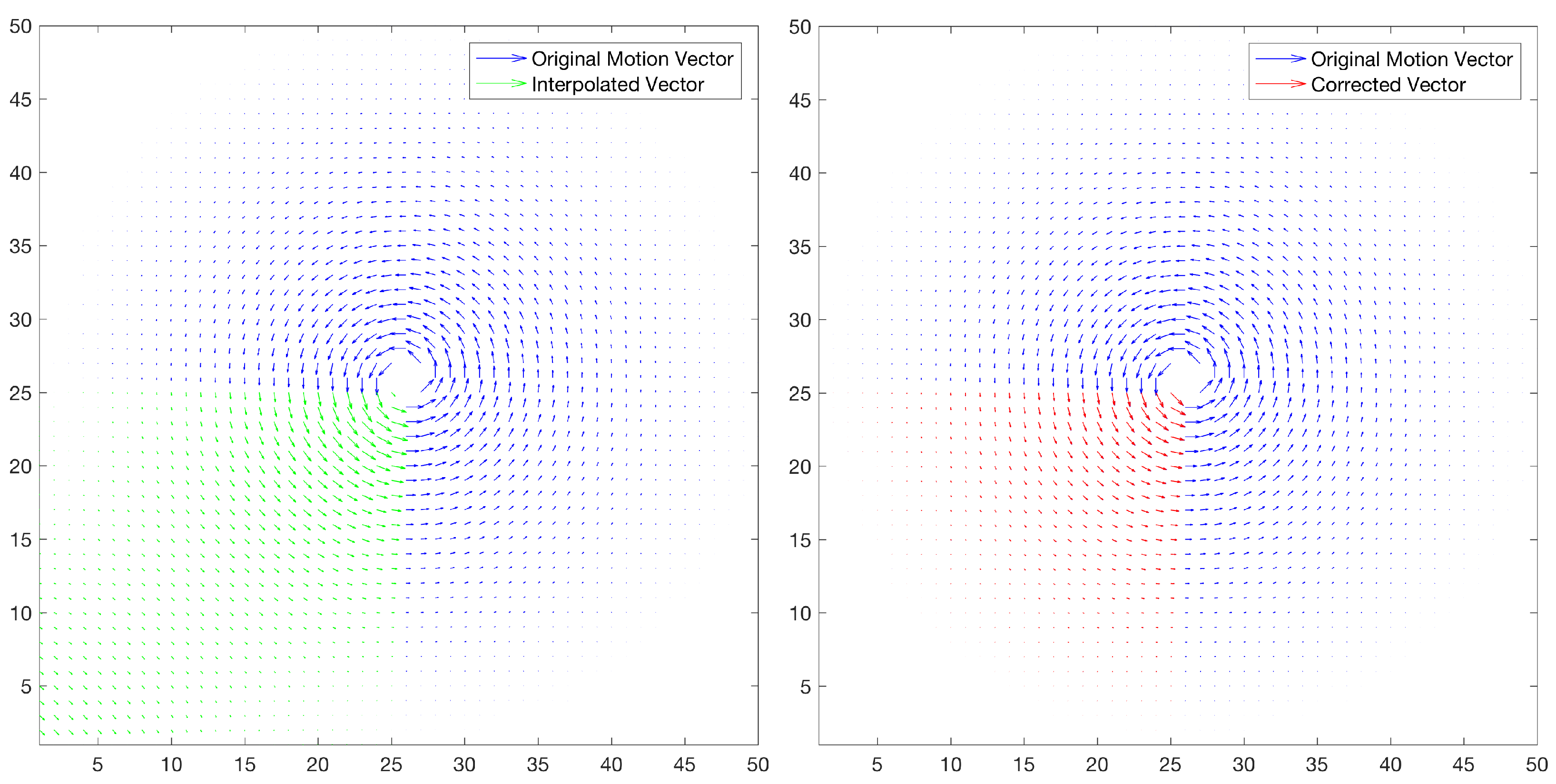
2.4. Motion Field Correction

The calculated and interpolated motion vector field from the previous step has the flaw that it may not follow a basic characteristic of the atmosphere, which is that the atmosphere is continuous and smooth. To get a realistic motion vector field from the obtained field, we add an optimization step to smooth the obtained motion field.In this study, we create a function with two penalties, a continuity penalty $J_C$ [17] and a smoothness penalty $J_S$. The cost function to be minimized is:

$$\begin{array}{cc}\hfill J(u,v)& =J_0+J_C+\alpha J_S\hfill \end{array}$$

(3)

$$\begin{array}{cc}\hfill J_0& ={\int }_{\Omega }\beta \left(\mathbf{x}\right)[{(u-u_0)}^2+{(v-v_0)}^2]\hfill \end{array}$$

(4)

u is the x-component of wind, and v is the y-component of the wind over the analytical domain $\Omega$, where $u_0$ and $v_0$ comprise the calculated motion vector from the previous step. The $\beta \left(\mathbf{x}\right)$ is the background error covariance that reflects the radar data quality at the location of $(x,y)$. For example, in the area where clutter and partial blockage of the radar beam often occurs, the weight will be lower. $J_0$ reflects the total differences between the final field and first guess field obtained in the previous step. The continuity term $J_C$, adopted from COTREC, is used to maintain mass conservation. In this scenario, we cannot enforce mass conservation everywhere in COTREC for two major reasons: (1) As COTREC is a single-radar algorithm, motion vectors on its domain boundary are often not zero; thus, it will allow a precipitation region to come inside and go outside of the domain; while in our scenario, vectors on boundaries are mostly $\mathbf{0}$, meaning that we do not expect precipitation to enter or leave the domain as we have mosaicked a large enough region to completely encompass the TC. (2) A TC often contains convective clouds with strong updraft and downdraft air flows; thus, across a fixed 2D altitude, mass may not be conserved. Thus, we impose a weak constraint on mass conservation so that the total mass in the analytical domain is conserved. This penalty term is:

$$\begin{array}{cc}\hfill J_C& ={\lambda }_C{D}^2\hfill \\ \hfill D& =\frac{\partial \rho u}{\partial x}+\frac{\partial \rho v}{\partial y}\hfill \\ \hfill {\lambda }_C& =\frac{1}{\Omega }{\left[{\int }_{\Omega }{(\frac{\partial \rho u}{\partial x}+\frac{\partial \rho v}{\partial y})}^{2}dxdy\right]}^{-1}\hfill \end{array}$$

(5)

Neglecting the compressibility over the analytical domain $\Omega$, $\rho$ will be a constant and can be discarded in $J_C$. The second term $J_S$ is the smooth penalty, adopted from [34,41], reported to be successful in the Korean radar network [42]. It is defined as:

$$J_S=\underset{\Omega }{\int \int }[{\left(\frac{{\partial }^{2}u}{\partial x^2}\right)}^2+2{\left(\frac{{\partial }^{2}u}{\partial x\partial y}\right)}^2+{\left(\frac{{\partial }^{2}u}{\partial y^2}\right)}^2+{\left(\frac{{\partial }^{2}v}{\partial x^2}\right)}^2+2{\left(\frac{{\partial }^{2}v}{\partial x\partial y}\right)}^2+{\left(\frac{{\partial }^{2}v}{\partial y^2}\right)}^2]dxdy$$

(6)

Finally, $J_S$ is scaled by $\alpha$, a constant factor. A previous study [43] shows that ${\nabla }^{2}J(u,v)$’s smallest eigenvalue is larger than the unit value of 1 (i.e., $J(u,v)$ is positive definite); thus, there exists a global minimal solution that can be solved by the conjugate gradient method. During the experiments, we found that since our first guess is close to the global minimal point, thus a quasi-Newton method like limited-memory Broyden–Fletcher–Goldfarb-Shannon (L-BFGS) usually converges very fast. Figure 3 shows how the minimized cost function $J(u,v)$ restores an idealized, symmetric circulation from a large missing patch in the third quadrant. The left panel shows interpolated (green) components from existing motion vector (blue), and the right panel shows restored components (right) using the smoothing. It is obvious that the proposed method can restore the original symmetrical pattern in the circular flow.

2.5. Advection Scheme

Once the final motion field is obtained, it is taken as unchanged for the entire forecast stage. TREC-based nowcasting methods usually use linear extrapolation during the entire period [3]. In fluid dynamics, this is called Eulerian advection, written as:

$$\mathbf{a}=\tau \mathbf{u}(t_0,\mathbf{x})$$

(7)

Linear extrapolation assumes all cloud structures keep their newest status and move along straight lines during the entire forecasting period. Since the assumption of linear movement breaks a basic physical fact that the atmosphere is a non-linear system, it cannot realistically account for nonlinear changes in the atmosphere. As a result, linear extrapolation only produces reliable predictions for a short amount of time, in which non-linearity can be neglected, often around 30–60 min. After that, errors become significant [44]. Through experiments, we confirm that linear extrapolation is not suitable for use in a TC scenario where winds have a tangential component to their motion. For a simple example, if rotation is neglected in a mature hurricane whose motion vectors are almost tangential, advecting the vectors linearly will tear the hurricane into pieces, leading to unreliable results in about 30 min. Later researchers reported using Lagrangian advection [45,46,47], which is effectively moving each pixel along its track according to the motion field. The scheme can adopt rotation and curved tracks, but it has a problem in that the final position of a pixel usually does not fall exactly on the center of grid cell, but instead overlaps with grid lines. Further, multiple pixels may partially overlap each other at the destination. Questions arise as to how to properly handle those unaligned pixels and partially overlapped areas given that rain drop size distribution information is not available inside each pixel. Hence, we choose to use a semi-Lagrangian scheme to convert a common extrapolation to an implicit extrapolation.

The semi-Lagrangian scheme is initially presented by [48] and further developed by [49] and refined by [23]. It is widely applied in trajectory models, for example, it is used in the HYSPLIT model from the National Oceanic and Atmospheric Administration (NOAA) [50]. In a semi-Lagrangian scheme, we choose a pixel at time $t_0+\tau$ and try to traverse back to $t_0$ with a time step of $\Delta t$ in order to see from whence it comes. Just like the Lagrangian scheme, its source “destination” may not fall on an exact cell center, and its nearest 8 neighbors within a 6-km buffer zone (two-cell-sized buffer zone) are selected to interpolate to such a value. Since we start from the endpoint in the semi-Lagrangian scheme, it is unclear what the momentum of the tracked air parcel is at the very beginning, we need iterative steps to determine the final displacement vector from its source to current endpoint:

$$\mathbf{a}=\sum _{i=1}^N\Delta t{\mathbf{u}}_{\mathbf{i}}(t_i,{\mathbf{x}}_{\mathbf{i}}-\frac{\mathbf{a}}{2})$$

(8)

where $\Delta t$ is the time step for iteration in which air parcels are advected linearly and $\mathbf{u}(t,\mathbf{x})$ is the motion vector at position $\mathbf{x}$, time t. Since we assume the motion field is static, we have $\mathbf{u}(t,\mathbf{x})=\mathbf{u}\left(t{,}_0\mathbf{x}\right)$. We found that the semi-Lagrangian scheme can converge very quickly in less than 3 iterations on the motion field obtained by Equation (3). Figure 4 shows the track for an air parcel from the position marked with the blue star as it moves inside towards the eye wall simulated by our semi-Lagrangian scheme. We choose to test it on an ideal stationary cyclone because we would like to avoid the external factors of the TC’s motion itself and interaction with surrounding weather systems in a real TC case. The ideal cyclone we set up is based on a climatological parameterization scheme presented by [51], whose radial wind profile is symmetric, and wind velocity generally decreases from the eye wall. Each pixel in Figure 4 is 20 km. The stationary cyclone has a circular eye with a radius of 20 km. We can clearly see that the air parcel comes from the outer bands and spirals into the eye wall. A very similar implementation can also be found in the mesocyclone detection and extrapolating algorithm from the Open Radar Product Generator (ORPG) in WSR-88D: The Common Operations and Development Environment (CODE) [52].

2.6. Determine the Source/Sink Term and Extrapolation

The source/sink term Q in Equation (1) represents the growth and decay of rainfall regions, which represents a major source of poor nowcasting if ignored [53]. In a Lagrangian or Euler extrapolation scheme, such growth and decay needs to be calculated over matched blocks between the last two consecutive images. However, in a semi-Lagrangian scheme, there is no need to trace and move blocks; it is simpler to calculate the rate of change of Q in each block along time. In this study, we calculate the average reflectivity change rate during the entire tracking period for mean reflectivity at each 4 × 4 block. This rate is also applied to any interpolated source pixels located in an adjacent 4 × 4 block.

3. Performance Evaluation

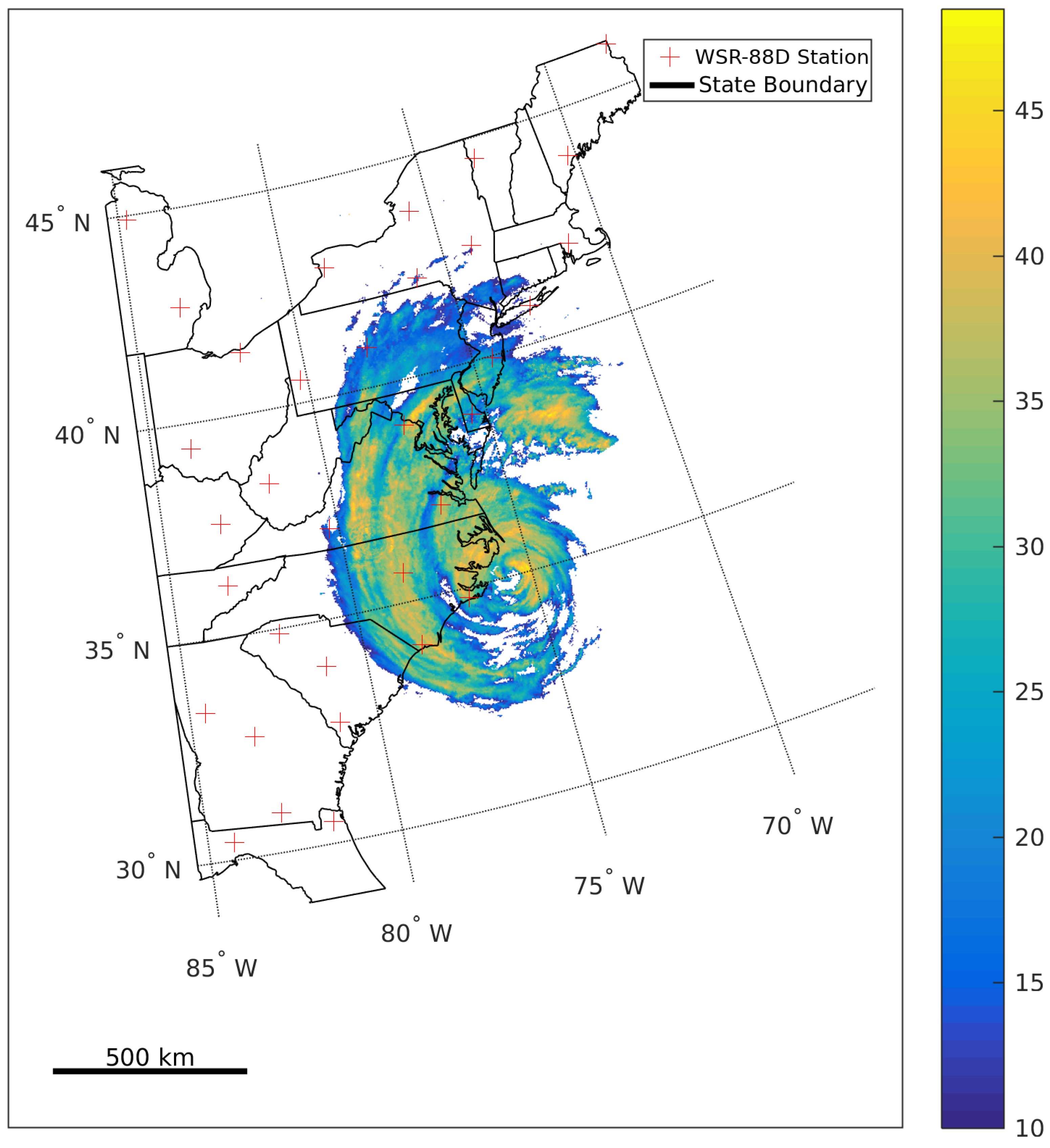
3.1. Data and Methods

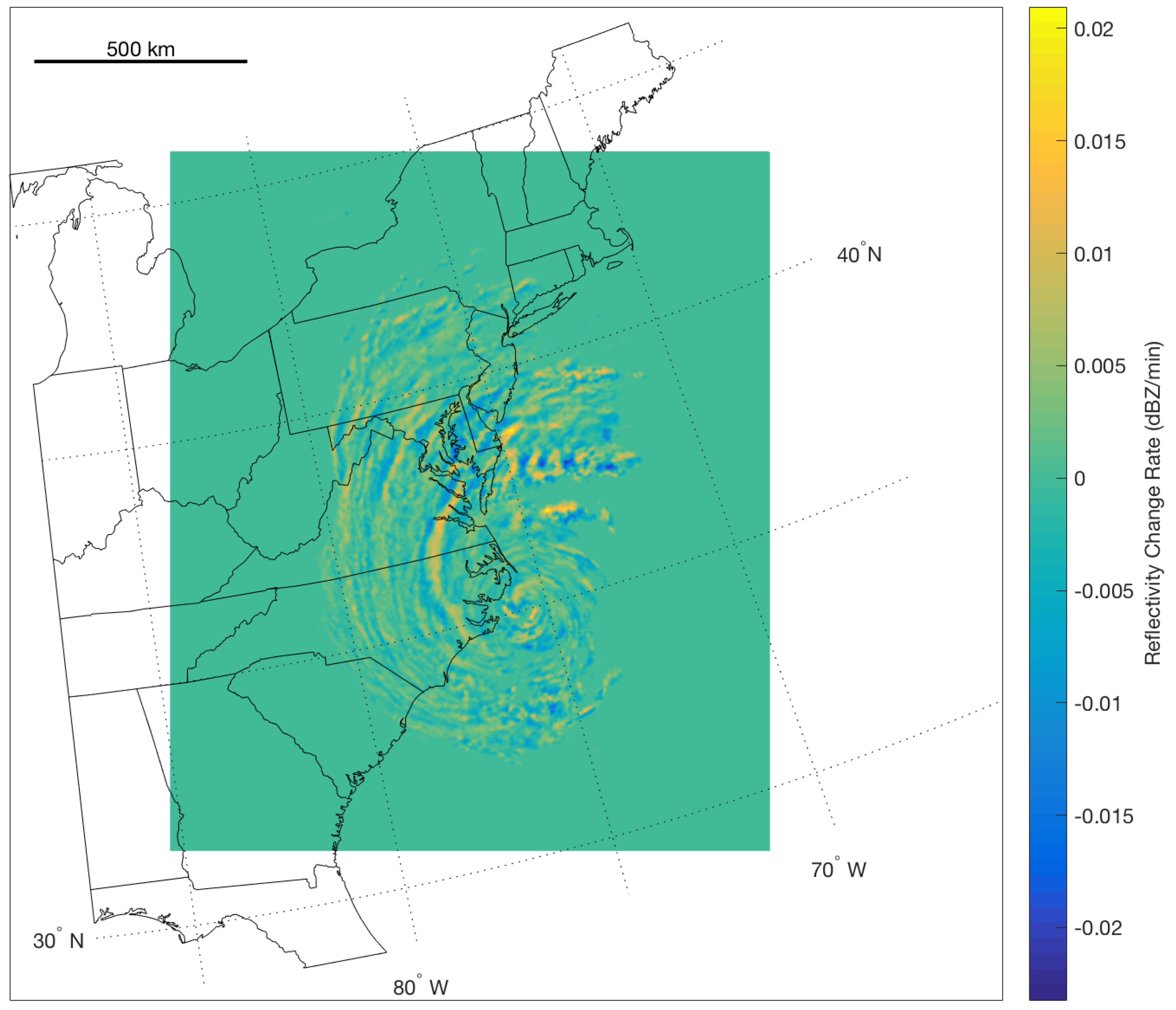
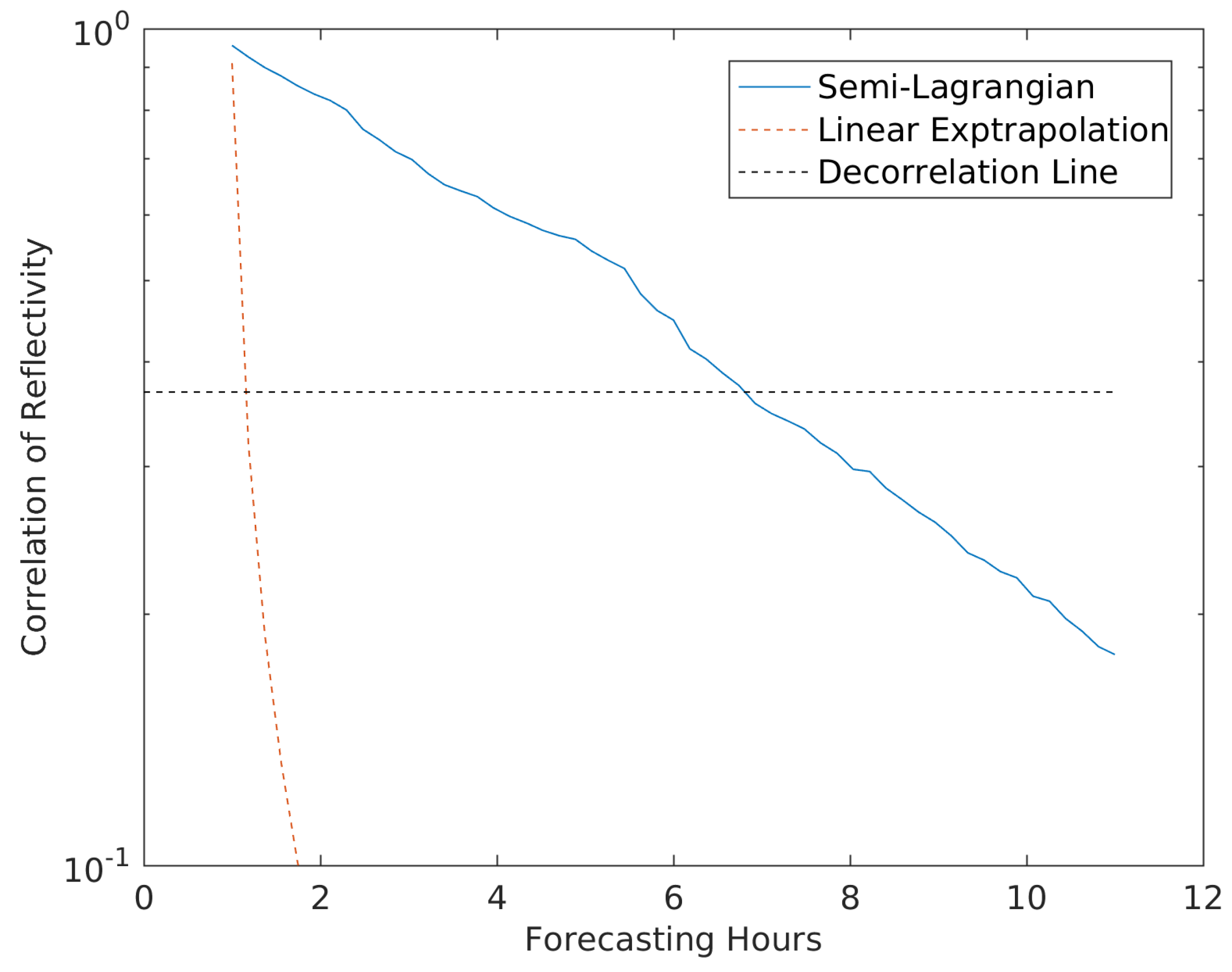
The case we present is Hurricane Isabel that made landfall over North Carolina in 2003 (Figure 5) [54]. We choose the Isabel case for the following reasons. First, the TC has a large and clearly-defined circulation center that allows convective clouds in the eye wall to be analyzed at 3-km resolution. Secondly, adequate radar reflectivity data are available for 36 h (from 18 September 2003 0900 UTC–19 September 2003 2100 UTC) while the storm was over land, leaving enough range to pick up one nowcasting event. Third, Isabel became restructured into a cold-cored low pressure system as it moved within radar range. Nearly half of Atlantic basin TCs experience this rapid change in structure [55], which causes rainfall regions to fragment and disperse from and dissipate behind the storm center [40,56]. Testing our model during Isabel’s restructuring process will allow us to evaluate the performance when a TC experiences changes in organization in both tangential and radial directions.

We create a time series of reflectivity mosaics from radar stations located within 600 km of the storm center. After removing non-meteorological echoes, data are gridded at a $3\times 3\times 0.5$ km spatial resolution and 10-min temporal resolution. In grid cells where multiple reflectivity values are available, we performed several experiments and determined that using the highest value from those available is the best solution, as we found that employing a weighted average algorithm leads to a low bias. This may be due to the fact that some stations have a slightly weaker signal [57]. Cells with missing values are filled using the Cressman interpolation [58]. Traditionally, quantitative precipitation estimation (QPE) is based on the composite reflectivity using a Z- R relationship [59]. However, recently, the work in [60] pointed out that using composite isothermal reflectivity below 0 °C instead of composite reflectivity in QPE improves the correlation in the Z-R relationship due to avoiding the overly high reflectivity values generated by melting hydrometeors around the freezing level [61]. Verification using the North American Regional Reanalysis (NARR) dataset, which has a reasonable representation of TC position and size over the U.S. [62], shows that the 0°C isotherm appears between the altitudes of 4.0 and 4.5 km over the entire analytical domain during the study period. Thus, a composite reflectivity is calculated using data below 4 km. Further, the composite reflectivity values are filtered with a low-pass filter with a 5 × 5 moving window. The filtered images are used for tracking, but we use original images to predict actual reflectivity values. The tracking stage is 0.5 h (e.g., 1730–1800 UTC), and the forecasting period is 8 h, with a 10-min resolution throughout the period. After that, we use the smoothing technique to obtain the final field. We set $\beta \left(\mathbf{x}\right)$ to I for the whole domain, which means that data quality is assumed to be the same over the domain. Because the Level-II data are quality controlled before mosaicking is performed, errors in data due to problems such as instrument errors are not a concern.

3.2. Results

Figure 6 shows the reflectivity change rate (source/sink term) Q determined during the tracking stage. Figure 7 shows a zoomed view near the inner core area from the final obtained motion field serving for forecasting. It is noticeable that the cloud rotation center is different from the eye, which is due to the velocity composition of Isabel’s movement and cloud rotation. When Isabel is moving toward northwest, the precipitation area on its left side (i.e., the southwest direction from the eye) will show the minimal velocity and rotation. In the outer area, it is clear that the field captured the rotation of Isabel. We also setup a base performance linear extrapolation experiment using traditional TREC and moving pixels linearly along motion vectors where pixels collocate.

Figure 8 shows the correlation between forecasting results and corresponding observed results. We find that the semi-Lagrangian advection scheme can produce reliable forecasts out to about 5 h before it falls to a decorrelation point defined as $R=\frac{1}{e}$ [63]. The reflectivity correlation drops linearly in the semi-logarithmic scale. This drop matches that in a previous study by [34], who stated that a good advection scheme should be able to maintain a consistent accuracy rate over the forecasting period. In other words, with a consistent accuracy rate, there should be an exponential drop over time, which shows a general linear relationship in a logarithmic scale. To evaluate the prediction success, we employ three standard scores used in operational radar-based nowcasting called contingency tables [64,65]. These scores are calculated by taking point by point comparisons at the prediction time between the value observed by the radar and the predicted value. If both the measured value and the predicted value are larger than a threshold, we consider the nowcast to be successful. If the measured value is larger than the threshold while the predicted value is smaller than the threshold, this is considered to be a failure. If the measured value is smaller than the threshold while the predicted value is larger than the threshold, this constitutes a false alarm. We chose to use 24 dBZ as the threshold as it roughly equals a 0.1-mm h${}^{-1}$ rain rate (about one inch daily) according to Rosenfeld’s Tropical Z-R relationship [66], while one inch over a day is generally considered a threshold with which to identify TC-related rainfall [67]. The contingency table contains three indices that are calculated based on three criteria, probability of detection (POD), false alarm ratio (FAR) and critical success index (CSI) [68]. Their equations are as follows:

$$POD=\frac{a}{a+b}$$

(9)

$$FAR=\frac{c}{a+c}$$

(10)

$$CSI=\frac{a}{a+b+c}$$

(11)

where a is the total pixels of successful nowcasting, b is failed nowcasting and c is false alarms. Figure 9 depicts the three skill scores over the prediction period. A roughly linear trend over time is observed for these CSI and POD scores, which also indicates a consistent hit rate for each step during the forecasting period. We also see FAR increase rapidly; this also matches patterns in previous research [23,34]. However, we can see that the semi-Lagrangian scheme outperforms linear extrapolation as the linear extrapolation can only produce a reliable prediction about 0.5–1 h.

4. Summary and Future Study

In this paper, a methodology is presented to forecast a TC’s rainfall distribution up to 8 h into the future using a high-resolution Doppler radar reflectivity mosaic in a large analytical domain. The method contains three steps to produce a reliable forecasting time series. First, a nested reflectivity motion vector retrieval method is designed. It uses the normalized 2D correlation between two reflectivity images to calculate motion vectors in a quad-tree pattern. Second, a numerical optimization technique creates a realistic motion field. This technique minimizes a cost function with three constraints: the residual of the reflectivity conservation equation, mass conservation over the entire domain and a smoothing penalty function. Finally a semi-Lagrangian scheme is designed to adopt three critical factors in nowcasting: mesoscale-sized circulations, momentum of air parcels and growth and dissipation of precipitation area. The results of the case study examining a landfalling hurricane with rapidly evolving rainfall regions shows that an acceptable prediction can be extended from the 1–2 h currently available in a single radar application to about 6 h in a multi-radar scenario.

Future research should extend this model from a deterministic model to a statistical model, which gives both the predicted value and uncertainty at the forecasting stage. This idea was reported in previous research [69] from a purely statistical aspect. It shows that a quantitative measurement of uncertainty improves accuracy in a small-scale storm, but a similar study on a large mesoscale system like a TC does not exist. Besides understanding uncertainty quantitatively for each forecasting time, measuring uncertainty and error spatially is also a potential topic to extend from this study. Furthermore, it is valuable to generate background covariance used in the optimization technique based on historical statistics on each station, rather than assigning a single value of one to all stations, in order to improve the accuracy of the smoothed motion field.

References

1. Rappaport, E.N. Loss of life in the United States associated with recent Atlantic tropical cyclones. Bull. Am. Meteorol. Soc. 2000, 81, 2065–2073. [Google Scholar] [CrossRef]
2. Rappaport, E.N. Fatalities in the United States from Atlantic tropical cyclones: New data and interpretation. Bull. Am. Meteorol. Soc. 2014, 95, 341–346. [Google Scholar] [CrossRef]
3. Wilson, J.W.; Crook, N.A.; Mueller, C.K.; Sun, J.; Dixon, M. Nowcasting thunderstorms: A status report. Bull. Am. Meteorol. Soc. 1998, 79, 2079–2099. [Google Scholar] [CrossRef]
4. World Meteorological Organization. Nowcast. Available online: http://www.wmo.int/pages/prog/amp/pwsp/Nowcasting.htm (accessed on 1 May 2018).
5. Cao, M.; Wei, J. Weather derivatives valuation and market price of weather risk. J. Futures Mark. 2004, 24, 1065–1089. [Google Scholar] [CrossRef]
6. Crum, T.D.; Alberty, R.L. The WSR-88D and the WSR-88D operational support facility. Bull. Am. Meteorol. Soc. 1993, 74, 1669–1687. [Google Scholar] [CrossRef]
7. Istok, M.J.; Fresch, M.; Smith, S.; Jing, Z.; Murnan, R.; Ryzhkov, A.; Krause, J.; Jain, M.; Ferree, J.; Schlatter, P.; et al. WSR-88D dual polarization initial operational capabilities. In Proceedings of the 25th Conference on Interactive Information and Processing Systems for Meteorology, Oceanography, and Hydrology, Phoenix, AZ, USA, 11–15 January 2009; American Meteorological Society: Boston, MA, USA, 2009; Volume 15. [Google Scholar]
8. Liang, Q.; Feng, Y.; Deng, W.; Hu, S.; Huang, Y.; Zeng, Q.; Chen, Z. A composite approach of radar echo extrapolation based on TREC vectors in combination with model-predicted winds. Adv. Atmos. Sci. 2010, 27, 1119–1130. [Google Scholar] [CrossRef]
9. Benjamin, S.G.; Weygandt, S.S.; Brown, J.M.; Hu, M.; Alexander, C.R.; Smirnova, T.G.; Olson, J.B.; James, E.P.; Dowell, D.C.; Grell, G.A.; et al. A North American hourly assimilation and model forecast cycle: The Rapid Refresh. Mon. Weather Rev. 2016, 144, 1669–1694. [Google Scholar] [CrossRef]
10. Sun, J. Convective-scale assimilation of radar data: progress and challenges. Q. J. R. Meteorol. Soc. 2005, 131, 3439–3463. [Google Scholar] [CrossRef]
11. Lakshmanan, V.; Humphrey, T.W. A MapReduce technique to mosaic continental-scale weather radar data in real-time. IEEE J. Sel. Top. Appl. Earth Obs. Remote Sens. 2014, 7, 721–732. [Google Scholar] [CrossRef]
12. Koch, S.E.; Ferrier, B.; Stoelinga, M.T.; Szoke, E.; Weiss, S.J.; Kain, J.S. The use of simulated radar reflectivity fields in the diagnosis of mesoscale phenomena from high-resolution WRF model forecasts. In Proceedings of the 11th Conference on Mesoscale Processes, Albuquerque, NM, USA, 24–29 October 2005; American Meteorological Society: Boston, MA, USA, 2005; Volume 7. [Google Scholar]
13. Ulbrich, C.W. Natural variations in the analytical form of the raindrop size distribution. J. Clim. Appl. Meteorol. 1983, 22, 1764–1775. [Google Scholar] [CrossRef]
14. Matyas, C.J.; Zick, S.E.; Tang, J. Using an object-based approach to quantify the spatial structure of reflectivity regions in Hurricane Isabel (2003): Part I: Comparisons between radar observations and model simulations. Mon. Weather Rev. 2018, 146, 1319–1340. [Google Scholar] [CrossRef]
15. Rinehart, R.; Garvey, E. Three-dimensional storm motion detection by conventional weather radar. Nature 1978, 273, 287–289. [Google Scholar] [CrossRef]
16. Tuttle, J.D.; Foote, G.B. Determination of the boundary layer airflow from a single Doppler radar. J. Atmos. Ocean. Technol. 1990, 7, 218–232. [Google Scholar] [CrossRef]
17. Li, L.; Schmid, W.; Joss, J. Nowcasting of motion and growth of precipitation with radar over a complex orography. J. Appl. Meteorol. 1995, 34, 1286–1300. [Google Scholar] [CrossRef]
18. Tuttle, J.; Gall, R. A single-radar technique for estimating the winds in tropical cyclones. Bull. Am. Meteorol. Soc. 1999, 80, 653–668. [Google Scholar] [CrossRef]
19. Mecklenburg, S.; Joss, J.; Schmid, W. Improving the nowcasting of precipitation in an Alpine region with an enhanced radar echo tracking algorithm. J. Hydrol. 2000, 239, 46–68. [Google Scholar] [CrossRef]
20. Gamba, P.; Dell Acqua, F.; Houshmand, B. SRTM data characterization in urban areas. Int. Arch. Photogramm. Remote Sens. Spat. Inf. Sci. 2002, 34, 55–58. [Google Scholar]
21. Zhang, Y.; Chen, M.; Xia, W.; Cui, Z.; Yang, H. Estimation of weather radar echo motion field and its application to precipitation nowcasting. Acta Meteorol. Sin. 2006, 64, 631–646. [Google Scholar]
22. Wang, G.; Wong, W.; Liu, L.; Wang, H. Application of multi-scale tracking radar echoes scheme in quantitative precipitation nowcasting. Adv. Atmos. Sci. 2013, 30, 448–460. [Google Scholar] [CrossRef]
23. Turner, B.; Zawadzki, I.; Germann, U. Predictability of precipitation from continental radar images. Part III: Operational nowcasting implementation (MAPLE). J. Appl. Meteorol. 2004, 43, 231–248. [Google Scholar] [CrossRef]
24. Harasti, P.R.; McAdie, C.J.; Dodge, P.P.; Lee, W.C.; Tuttle, J.; Murillo, S.T.; Marks, F.D., Jr. Real-time implementation of single-Doppler radar analysis methods for tropical cyclones: Algorithm improvements and use with WSR-88D display data. Wea. Forecast. 2004, 19, 219–239. [Google Scholar] [CrossRef]
25. Wang, M.; Zhao, K.; Wu, D. The T-TREC technique for retrieving the winds of landfalling typhoons in China. Acta Meteorol. Sin. 2011, 25, 91–103. [Google Scholar] [CrossRef]
26. Li, X.; Ming, J.; Wang, Y.; Zhao, K.; Xue, M. Assimilation of T-TREC-retrieved wind data with WRF 3DVAR for the short-term forecasting of typhoon Meranti (2010) near landfall. J. Geophys. Res. Atmos. 2013, 118. [Google Scholar] [CrossRef]
27. Wang, M.; Xue, M.; Zhao, K.; Dong, J. Assimilation of T-TREC-retrieved winds from single-Doppler radar with an ensemble Kalman filter for the forecast of Typhoon Jangmi (2008). Mon. Weather Rev. 2014, 142, 1892–1907. [Google Scholar] [CrossRef]
28. Wang, M.; Xue, M.; Zhao, K. The impact of T-TREC-retrieved wind and radial velocity data assimilation using EnKF and effects of assimilation window on the analysis and prediction of Typhoon Jangmi (2008). J. Geophys. Res. Atmos. 2016, 121, 259–277. [Google Scholar] [CrossRef]
29. Jorgensen, D.P. Mesoscale and convective-scale characteristics of mature hurricanes. Part II. Inner core structure of Hurricane Allen (1980). J. Atmos. Sci. 1984, 41, 1287–1311. [Google Scholar] [CrossRef]
30. Matyas, C.J. A geospatial analysis of convective rainfall regions within tropical cyclones after landfall. Int. J. Appl. Geospat. Res. 2010, 1, 71–91. [Google Scholar] [CrossRef]
31. Zhou, Y.; Matyas, C.J. Spatial characteristics of storm-total rainfall swaths associated with tropical cyclones over the Eastern United States. Int. J. Climatol. 2017, 37, 557–569. [Google Scholar] [CrossRef]
32. Jiang, H.; Liu, C.; Zipser, E.J. A TRMM-based tropical cyclone cloud and precipitation feature database. J. Appl. Meteorol. Climatol. 2011, 50, 1255–1274. [Google Scholar] [CrossRef]
33. Villarini, G.; Smith, J.A.; Baeck, M.L.; Marchok, T.; Vecchi, G.A. Characterization of rainfall distribution and flooding associated with U.S. landfalling tropical cyclones: Analyses of Hurricanes Frances, Ivan, and Jeanne (2004). J. Geophys. Res. 2011, 116. [Google Scholar] [CrossRef]
34. Germann, U.; Zawadzki, I. Scale-dependence of the predictability of precipitation from continental radar images. Part I: Description of the methodology. Mon. Weather Rev. 2002, 130, 2859–2873. [Google Scholar] [CrossRef]
35. Tang, J.; Matyas, C.J. Fast playback framework for analysis of ground-based Doppler radar observations using MapReduce technology. J. Atmos. Ocean. Technol. 2016, 33, 621–634. [Google Scholar] [CrossRef]
36. Pierce, C.; Ebert, E.; Seed, A.; Sleigh, M.; Collier, C.; Fox, N.; Donaldson, N.; Wilson, J.; Roberts, R.; Mueller, C. The nowcasting of precipitation during Sydney 2000: an appraisal of the QPF algorithms. Weather Forecast. 2004, 19, 7–21. [Google Scholar] [CrossRef]
37. Staniforth, A.; Côté, J. Semi-Lagrangian integration schemes for atmospheric models—A review. Mon. Weather Rev. 1991, 119, 2206–2223. [Google Scholar] [CrossRef]
38. Finkel, R.A.; Bentley, J.L. Quad trees a data structure for retrieval on composite keys. Acta Inform. 1974, 4, 1–9. [Google Scholar] [CrossRef]
39. Matyas, C. Shape measures of rain shields as indicators of changing environmental conditions in a landfalling tropical storm. Meteorol. Appl. 2008, 15, 259–271. [Google Scholar] [CrossRef]
40. Zick, S.E.; Matyas, C.J. A shape metric methodology for studying the evolving geometries of synoptic-scale precipitation patterns in Tropical Cyclones. Ann. Assoc. Am. Geogr. 2016, 106, 1217–1235. [Google Scholar] [CrossRef]
41. Wahba, G.; Wendelberger, J. Some new mathematical methods for variational objective analysis using splines and cross validation. Mon. Weather Rev. 1980, 108, 1122–1143. [Google Scholar] [CrossRef]
42. Bellon, A.; Zawadzki, I.; Kilambi, A.; Lee, H.C.; Lee, Y.H.; Lee, G. McGill algorithm for precipitation nowcasting by lagrangian extrapolation (MAPLE) applied to the South Korean radar network. Part I: Sensitivity studies of the Variational Echo Tracking (VET) technique. Asia-Pac. J. Atmos. Sci. 2010, 46, 369–381. [Google Scholar] [CrossRef]
43. Gao, J.; Nuttall, C.; Gilreath, C. Multiple Doppler wind analysis and assimilation via 3DVAR using simulated observations of the Planned Case Network and WSR-88D radars. In Proceedings of the 32nd Conference Radar Meteorology, Albuquerque, NM, USA, 23–29 October 2005; American Meteorological Society: Boston, MA, USA, 2005. [Google Scholar]
44. Wilson, J.W.; Mueller, C.K. Nowcasts of thunderstorm initiation and evolution. Weather Forecast. 1993, 8, 113–131. [Google Scholar] [CrossRef]
45. Berenguer, M.; Sempere-Torres, D.; Pegram, G.G. SBMcast–An ensemble nowcasting technique to assess the uncertainty in rainfall forecasts by Lagrangian extrapolation. J. Hydrol. 2011, 404, 226–240. [Google Scholar] [CrossRef]
46. Mandapaka, P.V.; Germann, U.; Panziera, L.; Hering, A. Can Lagrangian extrapolation of radar fields be used for precipitation nowcasting over complex Alpine orography? Weather Forecast. 2012, 27, 28–49. [Google Scholar] [CrossRef]
47. Zahraei, A.; Hsu, K.L.; Sorooshian, S.; Gourley, J.; Lakshmanan, V.; Hong, Y.; Bellerby, T. Quantitative precipitation nowcasting: A Lagrangian pixel-based approach. Atmos. Res. 2012, 118, 418–434. [Google Scholar] [CrossRef]
48. Sawyer, J. A semi-Lagrangian method of solving the vorticity advection equation. Tellus 1963, 15, 336–342. [Google Scholar] [CrossRef]
49. Robert, A. A stable numerical integration scheme for the primitive meteorological equations. Atmos. Ocean 1981, 19, 35–46. [Google Scholar] [CrossRef]
50. Stein, A.; Draxler, R.R.; Rolph, G.D.; Stunder, B.J.; Cohen, M.; Ngan, F. NOAA’s HYSPLIT atmospheric transport and dispersion modeling system. Bull. Am. Meteorol. Soc. 2015, 96, 2059–2077. [Google Scholar] [CrossRef]
51. Chavas, D.R.; Lin, N.; Emanuel, K. A model for the complete radial structure of the tropical cyclone wind field. Part I: Comparison with observed structure. J. Atmos. Sci. 2015, 72, 3647–3662. [Google Scholar] [CrossRef]
52. Stumpf, G.J.; Witt, A.; Mitchell, E.D.; Spencer, P.L.; Johnson, J.; Eilts, M.D.; Thomas, K.W.; Burgess, D.W. The National Severe Storms Laboratory mesocyclone detection algorithm for the WSR-88D. Weather Forecast. 1998, 13, 304–326. [Google Scholar] [CrossRef]
53. Browning, K.A. Nowcasting; Academic Press: London, UK, 1982. [Google Scholar]
54. Lawrence, M.B.; Avila, L.A.; Beven, J.L.; Franklin, J.L.; Pasch, R.J.; Stewart, S.R. Atlantic hurricane season of 2003. Mon. Weather Rev. 2005, 133, 1744–1773. [Google Scholar] [CrossRef]
55. Hart, R.E.; Evans, J.L. A climatology of the extratropical transition of Atlantic tropical cyclones. J. Clim. 2001, 14, 546–564. [Google Scholar] [CrossRef]
56. Atallah, E.; Bosart, L.F.; Aiyyer, A.R. Precipitation distribution associated with landfalling tropical cyclones over the eastern United States. Mon. Weather Rev. 2007, 135, 2185–2206. [Google Scholar] [CrossRef]
57. Matyas, C.J. Use of ground-based radar for climate-scale studies of weather and rainfall. Geogr. Compass 2010, 4, 1218–1237. [Google Scholar] [CrossRef]
58. Cressman, G.P. An operational objective analysis system. Mon. Weather Rev. 1959, 87, 367–374. [Google Scholar] [CrossRef]
59. Jorgensen, D.P.; Willis, P.T. A Z-R relationship for hurricanes. J. Appl. Meteorol. 1982, 21, 356–366. [Google Scholar] [CrossRef]
60. Ping-Wah, L.; Wai-Kin, W.; Ping, C.; Hon-Yin, Y. An overview of nowcasting development, applications, and services in the Hong Kong Observatory. J. Meteorol. Res. 2014, 28, 859–876. [Google Scholar]
61. Austin, P.M.; Bemis, A.C. A quantitative study of the “bright band” in radar precipitation echoes. J. Meteorol. 1950, 7, 145–151. [Google Scholar] [CrossRef]
62. Zick, S.E.; Matyas, C.J. Tropical cyclones in the North American Regional Reanalysis: An assessment of spatial biases in location, intensity, and structure. J. Geophys. Res. Atoms. 2015, 120, 1651–1669. [Google Scholar] [CrossRef]
63. Zawadzki, I. Statistical properties of precipitation patterns. J. Appl. Meteorol. 1973, 12, 459–472. [Google Scholar] [CrossRef]
64. Doswell, C.A., III; Davies-Jones, R.; Keller, D.L. On summary measures of skill in rare event forecasting based on contingency tables. Weather Forecast. 1990, 5, 576–585. [Google Scholar] [CrossRef]
65. Schaefer, J.T. The critical success index as an indicator of warning skill. Weather Forecast. 1990, 5, 570–575. [Google Scholar] [CrossRef]
66. Rosenfeld, D.; Wolff, D.B.; Atlas, D. General probability-matched relations between radar reflectivity and rain rate. J. Appl. Meteorol. 1993, 32, 50–72. [Google Scholar] [CrossRef]
67. Groisman, P.Y.; Knight, R.W.; Karl, T.R. Changes in intense precipitation over the central United States. J. Hydrometeorol. 2012, 13, 47–66. [Google Scholar] [CrossRef]
68. Polger, P.D.; Goldsmith, B.S.; Przywarty, R.C.; Bocchieri, J.R. National Weather Service warning performance based on the WSR-88D. Bull. Am. Meteorol. Soc. 1994, 75, 203–214. [Google Scholar] [CrossRef]
69. Xu, K.; Wikle, C.K.; Fox, N.I. A kernel-based spatio-temporal dynamical model for nowcasting weather radar reflectivities. J. Am. Stat. Assoc. 2005, 100, 1133–1144. [Google Scholar] [CrossRef]
Figure 1. The procedure of the tracking stage. It takes four consecutive reflectivity images over 30 min with a 10-min interval. The tracking radar echo by correlation (TREC) motion vector is based on a nested TREC calculation scheme.
Atmosphere 09 00200 g001
Figure 2. Workflow of the prediction stage, which this study sets to 8 h with a 10-min time step.
Atmosphere 09 00200 g002
Figure 3. The smoothing step corrects the interpolated field (green in the left pane) to a realistic and symmetric field (red in the right pane). The units of x-axis and y-axis are array indices.
Atmosphere 09 00200 g003
Figure 4. Simulated track of an air parcel as it moves in a spiral trajectory into the eye wall of an idealized stationary hurricane using the semi-Lagrangian scheme. The units of x-axis and y-axis are array indices.
Atmosphere 09 00200 g004
Figure 5. Radar reflectivity at Isabel’s landfall on 1700 UTC 18 September 2003. It is a composite reflectivity below a 4-km altitude (below the freezing layer). WSR-88D, Weather Surveillance Radar-1988 Doppler.
Atmosphere 09 00200 g005
Figure 6. The source/sink term Q for the prediction period.
Atmosphere 09 00200 g006
Figure 7. A zoomed view for motion vectors in the inner core area with background of reflectivity Z. For visibility, vectors are shown at 16 × 16 block-size (48 km × 48 km) scale.
Atmosphere 09 00200 g007
Figure 8. Correlation as defined in Equation (2) between forecast and observation during the prediction period.
Atmosphere 09 00200 g008
Figure 9. Skill scores during the prediction period. CSI, critical success index; POD, probability of detection.
Atmosphere 09 00200 g009