Article

Effects of Urban Greenspace Patterns on Particulate Matter Pollution in Metropolitan Zhengzhou in Henan, China

1
Forestry College, Henan Agricultural University, 95 Wenhua Road, Zhengzhou 450002, China
2
School of Environment and Natural Resources, The Ohio State University, 2021 Coffey Road, Columbus, OH 43210, USA
3
OSU South Centers, The Ohio State University, 1864 Shyville Road, Piketon, OH 45661, USA
4
Institute of Geographic, Space Information Engineer University, Zhengzhou 450001, China
*
Authors to whom correspondence should be addressed.
These authors contributed equally to this work.
Atmosphere 2018, 9(5), 199; https://doi.org/10.3390/atmos9050199
Submission received: 2 April 2018 / Revised: 13 May 2018 / Accepted: 17 May 2018 / Published: 21 May 2018
(This article belongs to the Special Issue Air Quality in China: Past, Present and Future)

Abstract

:
This case study was conducted to quantify the effects of urban greenspace patterns on particle matter (PM) concentration in Zhengzhou, China by using redundancy and variation partitioning analysis. Nine air-quality monitoring stations (AQMS) were selected as the central points. Six distances of 1 km, 2 km, 3 km, 4 km, 5 km, and 6 km were selected as the side lengths of the squares with each AQMS serving as the central point, respectively. We found: (1) the fine size of PM (PM2.5) and coarse size of PM (PM10) among four seasons showed significant differences; during winter, the concentration of PM2.5 and PM10 were both highest, and PM2.5 and PM10 concentration in summer were lowest. (2) To effectively reduce the PM2.5 pollution, the percentage of greenspace, the differences in areas among greenspace patches, and the edge complexity of greenspace patches should be increased at distances of 2 km and 3 km. To effectively reduce PM10, the percentage of greenspace at a distance of 4 km, the edge density at distances of 2 km and 4 km, and the average area of greenspace patches at a distance of 1 km should be increased. (3) Greenspace pattern significantly affected PM2.5 at a distance of 3 km, and PM10 at a distance of 4 km. From shorter distance to longer distance, the proportion of variance explained by greenspace showed a decline–increase–decline–increase trend for PM2.5, and a decline–increase–decline trend for PM10. At shorter distances, the composition of greenspace was more effective in reducing the PM pollution, and the configuration of greenspace played a more important role at longer distances. The results should lead to specific guidelines for more cost-effective and environmentally sound greenspace planning.

1. Introduction

During the last 30 years, air pollution in China has become a major environmental issue, especially particulate matter (PM) pollution [1] due to rapid urbanization and dramatic growth in energy consumption [2]. Particulate matter refers to a solid and liquid mixture consisting of organic and inorganic substances in air [3]. PM can be classified into several different types according to its origin, chemical composition, and size [4]. The size of PM is typically classified as coarse (2.5–10 µm, PM10), fine (0.1–2.5 µm, PM2.5), and ultra-fine (≤0.1 µm) [4,5]. In the last two decades there has been extensive and increasing use of PM10 and PM2.5 which are usually considered harmful to human health [6,7,8].
Studies on PM are not only important for scientific discoveries, but also can be important for developing environmental policies. Some studies focused on the relationship between PM pollution and human health, linking PM pollution to dramatic increases in cardiovascular and respiratory illnesses, problems in pregnancy and child development, and even mortality [9,10,11,12].
Spatial distribution of PM of different sizes and their contributing factors at regional or national scale have been investigated in several countries [13,14,15,16,17]. Source apportionment of particles is another important research area focusing on characterization of various sources of fine-particulate air pollution [18,19].
Several measures for reducing PM pollution, such as using cleaner energy, transforming the pattern of economic growth [20], restricting driving [21], and joint efforts at regional or national level [20] have been studied and suggested in heavily polluted provinces in northern China.
The effect of greenspace on air pollution has been investigated by a few researchers in China and other countries [1,22,23,24,25]. Some studies described the effect of the particle-capturing capacities or particle-removal capacity of different tree species in urban ecosystems in China [1,22,23]. It was found that forest structures, especially the canopy density and leaf area index, showed a significant correlation with the PM2.5 concentration index, while tree size measured by diameter at breast height (DBH) showed a weak correlation [24]. Ji et al. indicated that cypress trees reduced the outdoor PM concentration more than pine trees, and higher tree planting densities were more effective in reducing PM pollution concentration than lower planting densities [25]. In the street canyon environment, tree parameters as crown height, leaf density, tree height and spacing have been found to affect air pollution, and the combination of trees and other solid barriers has combined benefits on local air quality [26]. High-level tree canopies led to deterioration in air quality compared to the open space, while low-level green infrastructure (hedges) improved air quality [27]. The aerodynamic effects of trees were shown to be much more important in improving air quality than the direct effects of PM deposition [28,29,30]. In addition, biogenic volatile organic compounds and pollens from vegetation may be other sources of pollutants and pollutant precursors [31].
However, the relationship between greenspace spatial patterns and PM pollution at different scales and how much the greenspace spatial patterns affect PM pollution need further investigation, which will improve the understanding of potential greenspace distribution impact on air quality. Zhengzhou was selected as the site for our case study since it is a large city of 7749 square kilometers with almost 10 million people in Henna. Furthermore, its PM pollution often ranked among the top 10 worst cities in China, and may potentially get much worse since it is one of the most important transportation hubs in China [22].
This study took the air monitor stations as the central points of square plots ranging from 1 km × 1 km to 6 km × 6 km (scales), and its objectives were to reveal the exact relationship between the spatial pattern of greenspace and PM concentration at multiple scales using the redundancy analysis method. Based on the literature, the contributions of this study are: (1) it compares the effects of spatial pattern on particle matter distribution at different scales; (2) it explores the role of greenspace composition and configuration in indicating particle matter concentration variation for Zhengzhou; (3) it provides suggestion for the greenspace planning of urban renewal in fast-developing cities as Zhengzhou.

2. Experiments

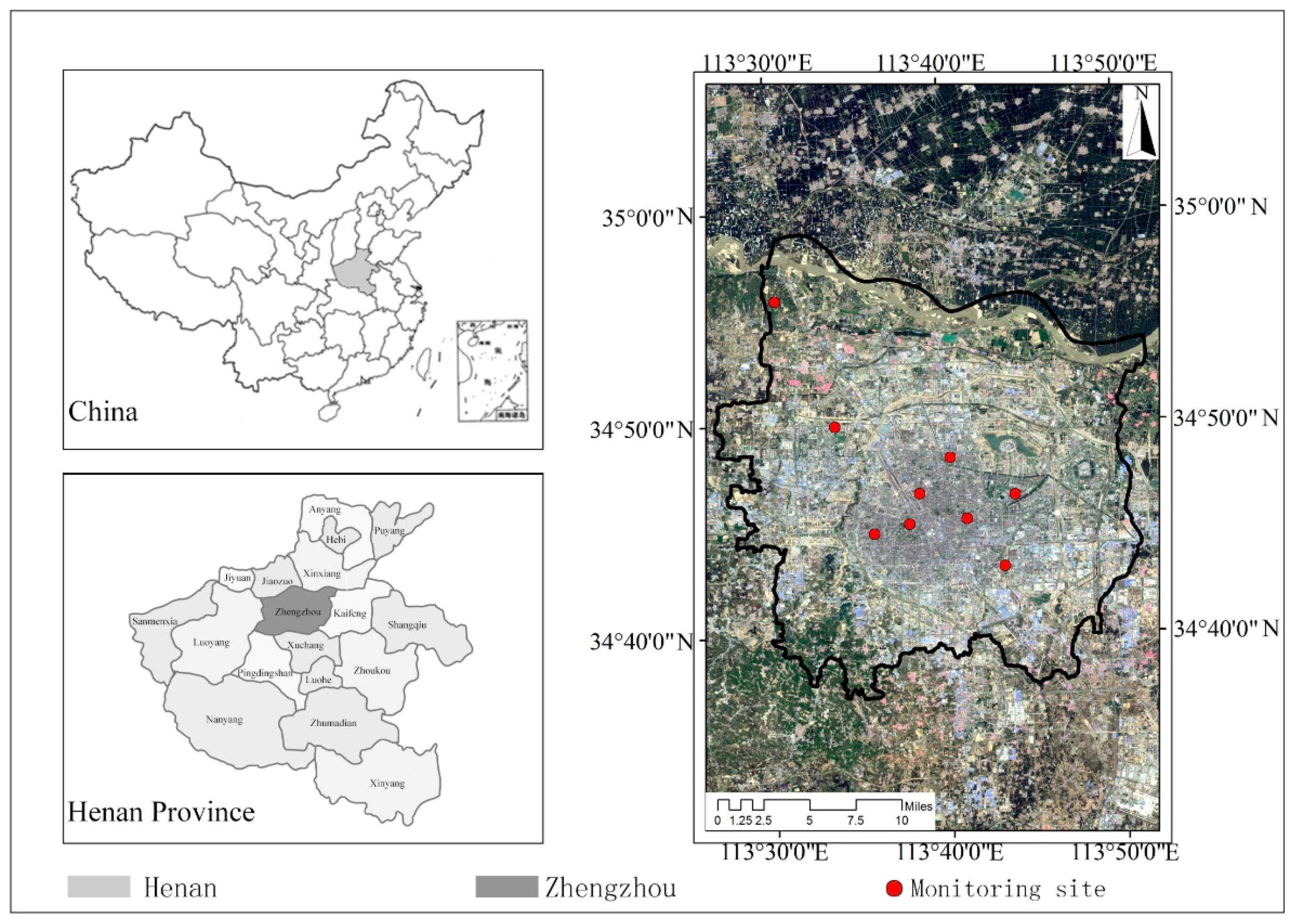
2.1. The Study Areas and Measurement Sites

Zhengzhou (34°16′ N–34°58′ N, 112°42′ E–114°14′ E) is the capital city of Henan Province in Central China and has four distinctive seasons. It is south of the North China Plain and the Yellow River (Figure 1). It is one of the largest transportation hubs in China. The population of the city was approximately 9.56 million according to the 2015 census (Henan Bureau of Statistics). The population density is the second highest in China. China lies mainly in the north-temperate zone, characterized by a mild climate and distinctive seasons, the nation can be sectored from south to north into equatorial, tropical, subtropical, warm-temperate, temperate, and cold-temperate zones according to temperature. Zhengzhou lies in the north warm-temperate zone, characterized by a warm climate and four distinctive seasons, with a dry spring (March–May), and a hot and rainy summer (June–September). The annual average temperature is 14–14.3 °C while the average annual precipitation is 640.9 mm. The total sunshine is 2400 h.

2.2. Data

2.2.1. PM2.5/10 Measurements

There are nine air-quality monitoring stations (AQMS) in Zhengzhou (Figure 1). These AQMS are located on rooftops. The building heights range from 3 to 15 m. The AQMS are located in similar areas with relatively few changes in land use. The sources of PM of the nine AQMS included dust particles from soil and roads, vehicle exhaust emission, fossil fuel combustion, and biomass burning. The AQMS are in Yanchang (YC) (34°45′0″ N, 113°40′48″ E) and Heyida (HYD) (34°45′0″ N, 113°38′24″ E) located in the business district, Zhengfangji (ZFJ) (34°46′12″ N, 113°38′24″ E) and Shijiancezhan (SJC) (34°45′0″ N, 113° 35′ 59.9994″ E) located in the residential area, Yinhangxuexiao (YHXX) (34°47′59.9994″ N, 113°40′12″ E), Gongshuigongsi (GSGS) (34°47′59.9994″ N, 113°33′36″ E), Jingkaiquguanwei (JKQ) (34°43′11.9994″ N, 113°43′48″ E) and Sishiqizhong (SSQ) (34°43′11.9994″ N, 113°43′38″ E) located in the cultural and educational area, while that at Ganglishuiku (GLSK) (34°55′12″ N, 113° 36′ 35.9994″ E) is in the suburban area.
Daily air-quality (PM2.5, PM10) data at nine AQMS from 1 January 2016 to 31 December 2016 were obtained from China National Environmental Monitoring Center (http://www.aqistudy.cn), and weather data were acquired from the Zhengzhou Bureau of Meteorology (http://www.zzqx.gov.cn). Air-quality data during rainy days were removed from the daily air-quality dataset. Based on the modified daily air-quality data, monthly averages were calculated. Twelve months in a year were divided into the four seasons, which are spring (March to May), summer (June to August), autumn (September to November), and winter (December to February). Average seasonal PM2.5 and PM10 concentrations of spring (PM2.5SP, PM10SP), summer (PM2.5SU, PM10SU) autumn (PM2.5AU, PM10AU) and winter (PM2.5WI, PM10WI) were calculated based on monthly averages, and the seasonal air-quality datasets were employed in the redundancy analysis (RDA).

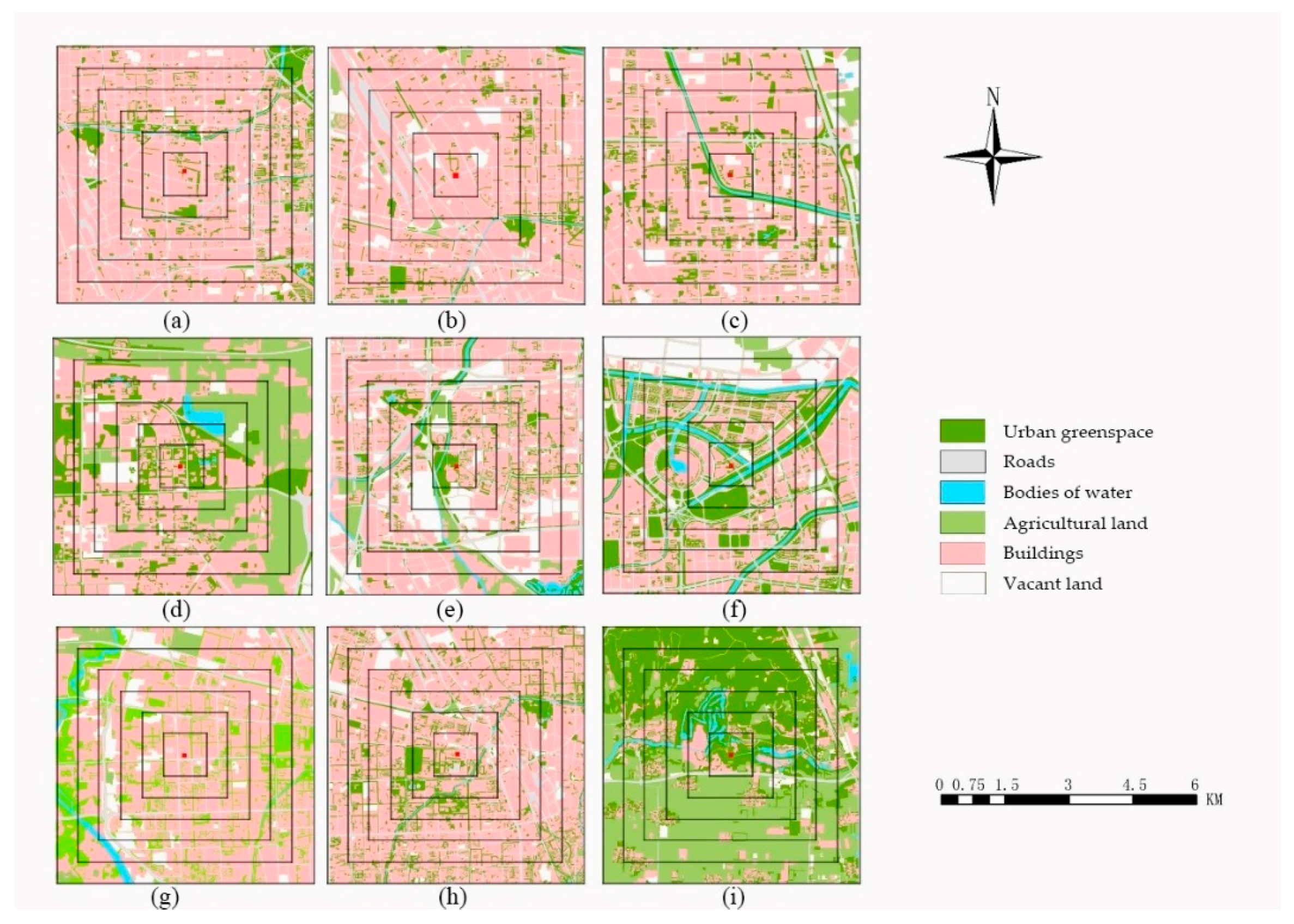
2.2.2. Greenspace Spatial Patterns

Remote-sensing images of high resolution were used to acquire the spatial patterns of urban greenspace as described in two previously published reports [32,33]; three types of greenspace maps with different spatial resolutions (2.44 m, 10 m, and 30 m) were used and were referred to as the Quickbird, SPOT, and TM images, respectively [32], the composition and configuration of land-cover features were measured by a series of landscape metrics based on a high-resolution land-cover map from aerial imagery [33]. In this study, we used the nine AQMS as the central points to create six square plots per site ranging in scale from 1 km × 1 km to 6 km × 6 km for each monitoring site (Figure 2). The smallest scale of our sample plots is 1 km × 1 km since this scale was shown to be highly suitable for the micro-scale research of urban forestry [34,35]. Quickbird images of the 6 km square buffers of all the monitoring sites were obtained in June 2016; the Quickbird images had one panchromatic band and four multispectral bands, with spatial resolution of 0.6 m and 2.4 m. To take advantage of both high resolutions and multispectral features, the multispectral bands were pan-sharpened using the panchromatic band from nine 6 km × 6 km scale images, with the principal components algorithm. Consequently, multispectral images were obtained with 0.6 m spatial resolution, and then geometric correction was performed with imagery from GoogleTM as the reference map [32,36]. The final images were used to map land cover in Zhengzhou, and then greenspace information was extracted from the land-cover data. A patch-based layer of different land cover types in vector format was created using object-based image analysis as used in several similar studies [33,36,37,38]. In this study, land-cover types included: (1) urban greenspace; (2) roads; (3) bodies of water; (4) agricultural land; (5) buildings; and (6) vacant land. The classification accuracies were checked based on 200 randomly selected points using reference data that were visually interpreted from the Google images. The verified classification accuracies were 91.5%.
Landscape metrics were widely used to describe greenspace patterns [39]. In this study, six class-level metrics were used to measure spatial patterns of urban greenspace. The spatial patterns (Table 1) included one composition metric and five configuration metrics: Percentage of landscape (PLAND) which quantified the proportional abundance of urban greenspace in multi-scale plots, and five metrics: mean patch size (AREA_MN) which equaled the sum of area across all patches in the greenspace divided by the total number of patches; mean patch shape index (SHAPE_MN) which was a measure of shape complexity; edge density (ED) which was a measure of edge length of greenspace divided by total greenspace area; largest patch index (LPI) which quantifies the percentage of total landscape area comprised by the largest patch, and it is a simple measure of greenspace dominance; and mean Euclidian nearest neighbor distance (ENN_MN) which is perhaps the simplest measure of patch context and has been used extensively to quantify patch isolation.
These metrics have been used in several papers published on the relationship between landscape patterns and ecological processes [32,34,40,41]. These metrics were chosen according to the following principles: (1) theoretically and practically important [33,38,42]; (2) easily calculated and explained; (3) little redundancy [33,37,40], the landscape metrics were obtained from the greenspace maps using the landscape structure analysis program FRAGSTATS for all of the plots [32].

2.3. Data Analysis

Three statistical methods were used in this study. First, we performed one-way analysis of variance (ANOVA) to examine whether there were significant differences among the PM2.5 and PM10 concentrations among the four seasons. We compared the PM2.5 and PM10 concentrations at the nine monitoring sites using the least significant difference (LSD) test, with significance level at p < 0.05. All values were reported as mean ± standard error (SE). the analyses were conducted using version 22.0 of SPSS software [43].
Second, we used the redundancy analysis (RDA) to investigate the relationship between the PM2.5/10 concentration and spatial patterns of the greenspace from scale 1 km × 1 km to scale 6 km × 6 km. RDA is a constrained ordination method that preserves the Euclidean distances among sites in the full dimensional space [44]. RDA has been the method of choice in determining the relationship between plant community and environment [45,46,47,48]. In this study, centralized and standardized transformation was conducted for the PM2.5 and PM10 data matrixes to maintain the integrity of PM data. In order to estimate the approximate significance of the relationship between the PM2.5 and PM10 data set and the spatial variables, we applied a Monte Carlo test with 1000 random permutations, assuming H0 as a non-linear relationship between the metrics [44]. There were eight datasets in total for the RDA and these included two response variables (PM2.5, PM10) datasets, and 6 explanatory variables (spatial pattern metrics from scale 1 km × 1 km to scale 6 km × 6 km) datasets. RDA was performed 12 times; 6 times employing the PM2.5 seasonal dataset as the response variables and metrics of 6 scales as explanatory variables, and another 6 times employing the PM10 dataset as the response variables and metrics of 6 scales as explanatory variables. These analyses were performed using the “Vegan Package” [49] in the R statistical language and environment.
Third, variance partitioning based on partial RDA was performed to assess the relative variance in PM2.5/10 of three groups of explanatory variables: (1) percentage of greenspace; (2) configuration of greenspace; (3) joint effects of composition and configuration metrics. Variance partitioning was performed by using “Spdep package” in R (version 2.4-4) [50].

3. Results

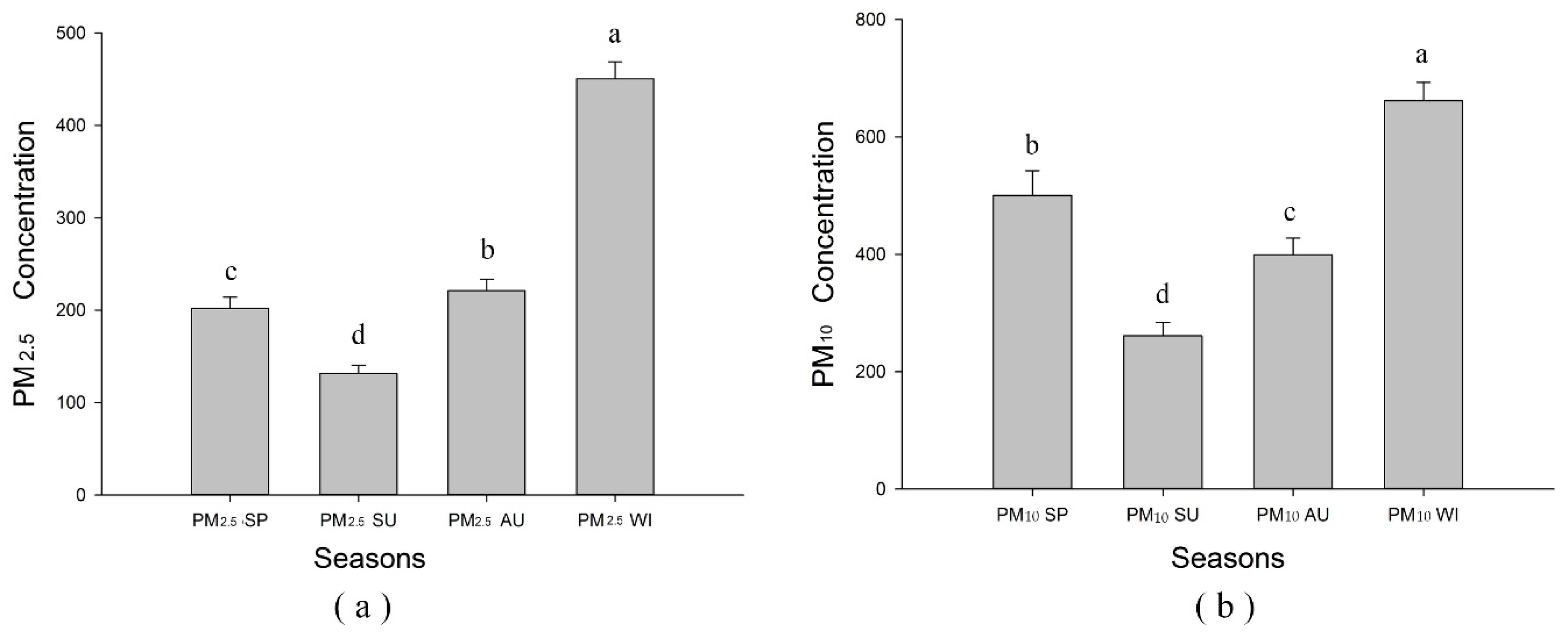
3.1. Seasonal Differences in Particulate Matter (PM) Pollution

The ANOVA analysis revealed significant differences (p < 0.05) among PM concentrations during four seasons (Figure 3). During winter, both PM2.5 and PM10 concentrations were highest while both PM2.5 and PM10 were lowest in summer. PM2.5 concentration in autumn was higher than that in spring while PM10 concentration in autumn was lower than that in spring (Figure 3).
Variations in air temperatures, humidity, wind direction and speed, presence and absence of leaves on vegetation, and fossil energy consumption patterns could all be possible reasons for the PM2.5 and PM10 concentrations fluctuating significantly during the four seasons. In winter, there is much more fossil energy consumption in northern China for keeping buildings warm, and most plant leaves fall off. These two factors lead to more primary and secondary PM pollutants. In summer, there is the highest vegetation coverage and much less consumption of fossil energy, thus very likely leading to less primary and secondary PM pollutants.

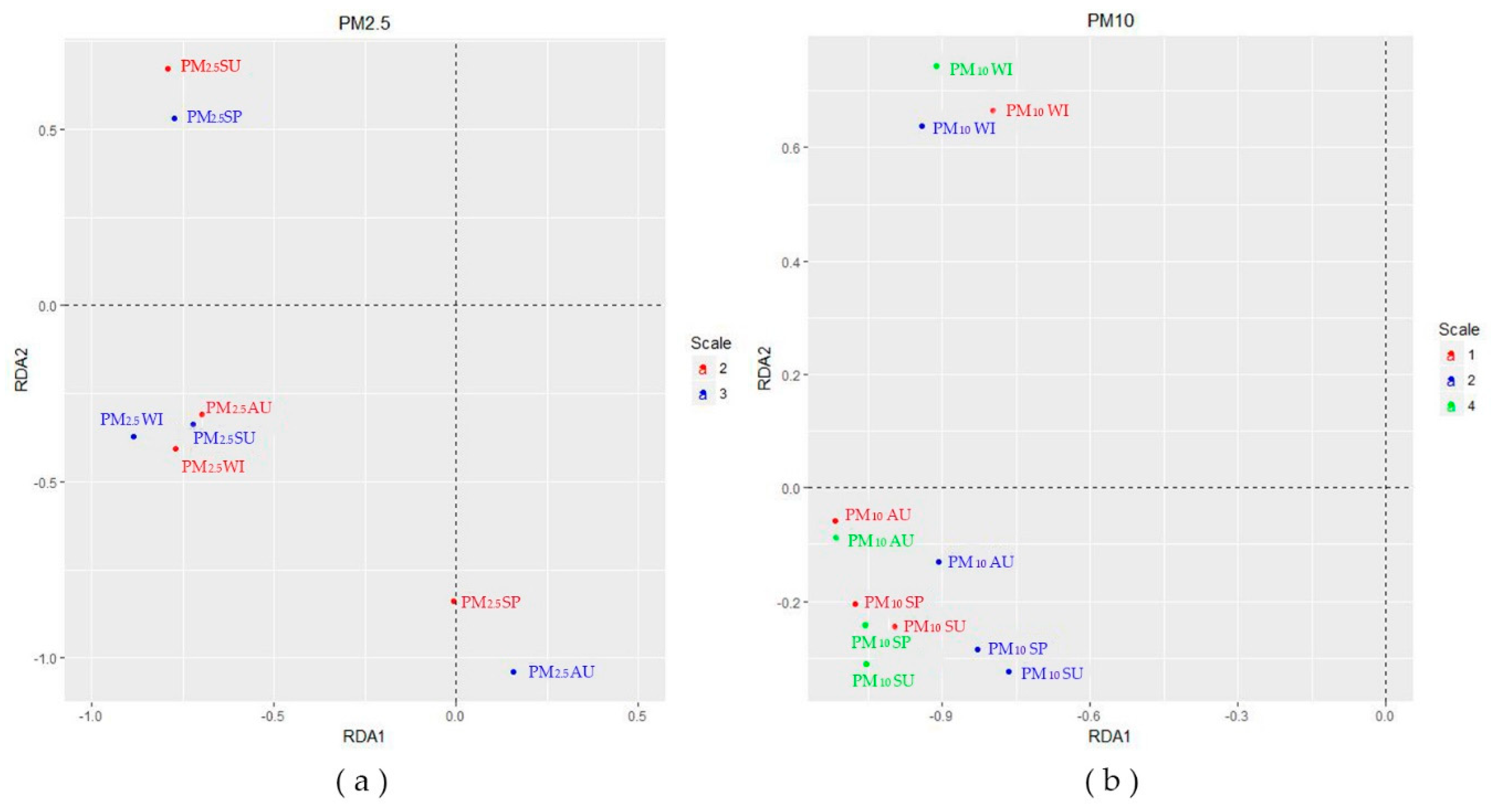
3.2. Redundancy Analysis (RDA)

Based on RDA, the cumulative proportions of total variance of the first two axes (PM2.5) from scale 1 to scale 6 were 0.5918, 0.5526, 0.6266, 0.5514, 0.5756 and 0.5843, respectively, and those of PM10 were 0.8004, 0.6345, 0.8165, 0.8862, 0.8418, 0.7506, respectively (Table 2). The proportion explained of variance means how much variance of PM pollution is explained by greenspace patterns at the first two RDA axes, and the cumulative proportion of variance is the sum of the first two RDA axes’ proportions of variance.
In Table 3, F-Ratio and p-value were used to test whether the multiscale greenspace patterns affected the PM pollution significantly, and R2 represented the variance of PM pollution explained by greenspace patterns in RDA model, and the R2adj was the adjusted or real value of the explained proportion. R2 of PM2.5 from scale 1 to scale 6 were 0.8342, 0.7407, 0.8848, 0.7679, 0.814, 0.8324, respectively, and R2 of PM10 from scale 1 km × 1 km to scale 6 km × 6 km were 0.89, 0.7155, 0.8922, 0.95445, 0.91193, 0.8219, respectively (Table 3). The Monte Carlo permutation tests indicated that the landscape metrics of greenspace of scale 3 and scale 4 significantly explained the total variance of PM2.5 and PM10 datasets, respectively. (Table 3). From scale 1 km × 1 km to 6 km × 6 km, the proportion of variance explained by the greenspace pattern (R2) showed a decline–increase–decline–increase trend with PM2.5, and a decline–increase–decline trend with PM10.
Each scale included six metrics: PLAND, LPI, ED, AREA_MN, SHAPE_MN and ENN_MN. With PM2.5, PLAND (negative), LPI (positive) and ED (positive) significantly related to the second axis of scale 2 km × 2 km and the first axis of scale 3 km × 3 km; PLAND, LPI and ED and the second axis of scale 3 km × 3 km (Table 4). With PM10, PLAND (negative) and AREA_MN (positive) significantly related to the first axis of scale 1 km × 1 km; ED (positive) significantly related to the first axis of scale 2 km × 2 km; PLAND (positive) and ED (negative) significantly related to the second axis of scale 4 km × 4 km.
The values in Table 4 showed the correlation between the greenspace patterns and the first two RDA axes of both PM2.5 and PM10 from scale 1 km × 1 km to 6 km × 6 km. Based on the correlation between landscape metrics and RDA axes above, we chose the scales, at which relationships between axis and PM concentration were significant in order to draw Figure 4. At scale1, PM10 of the four seasons negatively related to the first axis (Figure 4). At scale 2 km × 2 km, PM2.5SU had a positive relationship with the second axis, while PM2.5SP, PM2.5AU and PM2.5WI had negative relationships with the second axis; PM10 in the four seasons negatively related to the first axis (Figure 4). At scale 3 km × 3 km, PM2.5SP, PM2.5SU and PM2.5WI had negative relationships with the first axis apart from PM2.5AU, and PM2.5 of the whole year had negative relationships with the second axis except summer (Figure 4). At scale 4 km × 4 km, PM10 of the four seasons negatively related to the second axis except winter (Figure 4).
The relationship between greenspace patterns and PM concentrations was extrapolated based on the information in Table 4 and Figure 4. The PLAND of greenspace had positive relationship with PM2.5 except summer at scale 2 km × 2 km; PLAND had a positive relationship with part of the variance of PM2.5 except autumn, and negative relationship with part of the variance of PM2.5 in four seasons except spring at scale 3 km × 3 km; PLAND was positively related to PM10 at scale 1 km × 1 km; PLAND was positively related to PM10WI and negatively related to PM10 in other seasons at scale 4 km × 4 km.
LPI and ED of greenspace had a positive relationship with PM2.5SU, and a negative relationship with part of the variance of PM2.5 in the other seasons at scale 2 km × 2 km; LPI and ED had a negative relationship with part of the variance of PM2.5 except autumn and a positive relationship with the other part of the variance of PM2.5 except spring scale 3 km × 3 km. ED was negatively related to PM10 at scale 2 km × 2 km; ED was negatively related to part of the variance of PM10, and positively related to the other part of the variance of PM10 except winter at scale 4 km × 4 km. AREA_MN had a negative relationship with PM10 except in winter at scale 1 km × 1 km.

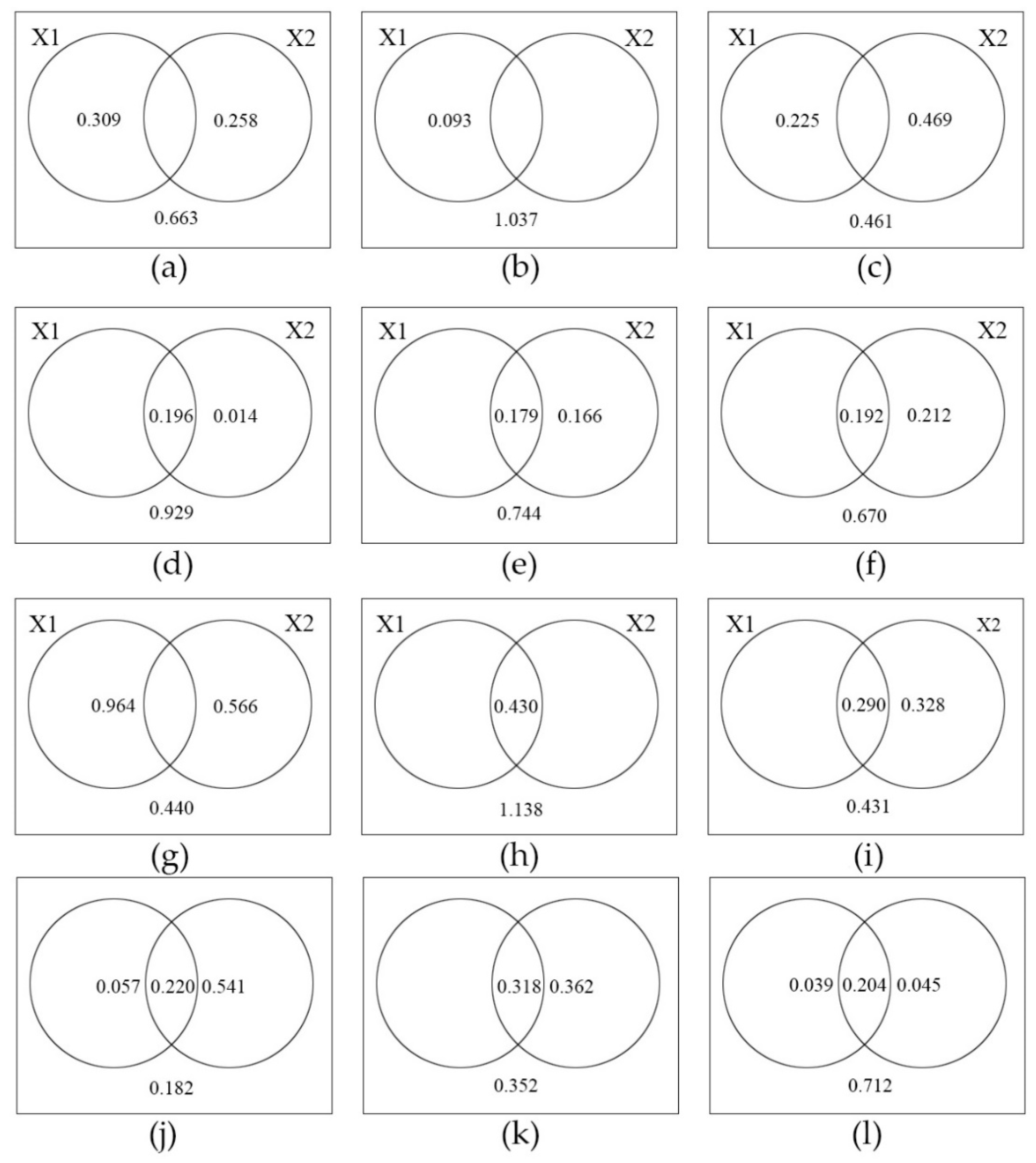
3.3. Variation Partitioning Analysis

Among the six scales, the Monte Carlo permutation test at scale 3 km × 3 km was significant (p < 0.05) and had the biggest explained variance to the PM2.5 dataset, and at scale 3 km ×3 km, 22.5% of the PM2.5 matrix is explained by a pure effect of the composition metric, 46.9% by a pure configuration metric, and about 46.1% of the variation remains unexplained. There is no common explained variance between composition and configuration metrics at small scale such as scale 1 km × 1 km, 2 km × 2 km and 3 km × 3 km, while common explained variance between both types of variables show up at large scale such as scale 4 km × 4 km,5 km × 5 km and 6 km × 6 km. Results from the variation partitioning also indicated that the configuration of greenspace played a more important role than that of percent cover of greenspace except scale 1 km × 1 km and 2 km × 2 km (Figure 5).
The Monte Carlo permutation test at scale 4 km × 4 km was significant (p < 0.01) and had the biggest explained variance to the PM10 dataset; 5.7% of the PM10 matrix is explained by a pure effect of the composition metric, 54.1% by a pure configuration metric, and 22% by composition and configuration metrics together. About 18.2% of the variation remains unexplained. There is common explained variance between composition and configuration metrics at all scales except scale 1 km × 1 km. As with the PM2.5 data, results from the variation partitioning also indicated that the configuration of greenspace played a more important role than that of percent cover of greenspace except at the scales 1 km × 1 km and 2 km × 2 km (Figure 5).

4. Discussion

4.1. Scale-Dependent Effects of Greenspace Pattern on PM Pollution

PM2.5/10 concentrations were significantly different among the four seasons in this study, and this finding was consistent with that in published papers on PM pollution in northern China [51,52]. Annual and seasonal average concentrations of PM had been used to investigate the effects of landscape pattern in another study [40], but the differences among seasons were quite significant. The multivariate statistical analysis method RDA helped in studying the effects of greenspace patterns on the PM pollution in much greater detail during the entire year, and the results should lead to better urban planning policies.
Based on our results, the landscape metrics (PLAND, LPI, ED and AREA_MN) showed significant effects on the first two RDA axes. The PLAND of greenspace reduced the PM2.5 concentration in summer at scale 2 km × 2 km, and reduced the PM10 concentration in spring, summer and autumn at scale 4 km × 4 km; the LPI and ED of greenspace reduced the PM2.5 concentration except summer at scale 2 km × 2 km, and reduced PM2.5 concentration in summer and winter at scale 3 km × 3 km, and the ED also reduced PM10 concentration in scale 2 km × 2 km and PM10WI at scale 4 km × 4 km; the AREA_MN reduced PM10 concentration except winter at scale 1 km × 1 km. However, the four metrics increased the PM concentrations during certain seasons at several scales.
Previous studies suggested that greenspace reduced PM2.5 concentration as a sink landscape [53], and outdoor PM2.5 concentrations can be reduced by dry and wet deposition on leaves; it was revealed that vegetation had the strong impact on PM2.5 mitigation [40], and a combination of trees and other solid barriers, such as building and parked cars, could reduce local air pollution [26], so higher PLAND of greenspace reduced more PM pollution. Higher LPI and ED may increase the interactions between greenspace and other elements in urban areas to mitigate PM pollution more efficiently, because LPI increased the energy gradient between greenspace and other elements and their interaction, and as an indicator of the complexity of the green space edges, ED reflects the degree of interactions between greenspace and other elements [40]. On the other hand, during some seasons in Zhengzhou, such as winter and early spring, there were no plants covering the soil surface, and the strong wind may lead to more dust particles in the air. During dry seasons such as autumn, increasing interaction between greenspace and other elements in urban areas by higher ED and LPI would lead to faster near-ground wind speed and increases in air humidity, and the strong wind may lead to higher PM concentration under higher humidity [54,55]. In addition, the aerodynamic effects of greenspace are stronger than the positive effects of deposition [28,29], and more trees in a street canyon may lead to a reduction of ventilation and an average increase of air pollution [28], and it was reported that high-level vegetation canopies (trees) led to a deterioration in air quality, while low-level green infrastructure (hedges) improved air-quality conditions [27]. The relationship between spatial patterns and PM concentration varied in different seasons and scales, and the landscape metrics of greenspace influenced PM concentration in both positive and negative manners, thus, the usefulness of greenspace in reducing PM concentration hinges on the balance between these pros and cons. To reduce the PM2.5 pollution, both scales and greenspace patterns should be considered during the urban planning and design process, and the percentage of greenspace should be increased at 2 km × 2 km and 3 km × 3 km scales. Increasing the area difference and edge complexity of greenspace patches at 2 km × 2 km and 3 km × 3 km scales should be an effective approach. To reduce PM10, we should increase the percentage of greenspace at the 4 km × 4 km scale, the edge densities at the 2 km × 2 km and 4 km × 4 km scales, and the average area of greenspace patches at the 1 km × 1 km scale. In addition, during winter and early spring, mitigation measures are still needed to keep dust particles contained within the greenspace; for example, landscape mulch, plant groundcovers and evergreen shrubs should be considered.

4.2. Scale-Dependent Variation Partitioning

Air PM pollution could be caused by many factors. It is well known that greenspace or vegetation reduces the PM pollution by increasing the deposition of PM, but there were no reports to identify the exact extent of greenspace patterns in explaining the variances of PM concentration. This study has improved the understanding of the scale-dependent correlation between PM pollution and greenspace patterns. Based on the results of our variation partitioning analysis, variance of PM2.5 and PM10 concentration explained by greenspace spatial patterns varied at different scales. Hence, the scale should be an important factor in determining the relationship between spatial pattern and ecological process. Most scales used in this study explained little variance according to the Monte Carlo permutation test, except scale 3 km × 3 km for PM2.5, and scale 4 km × 4 km for PM10. From scales 1 km × 1 km to 6 km × 6 km, the proportion of variance explained by greenspace spatial patterns showed a decrease–increase–decrease-increase trend for PM2.5, and a decrease–increase–decline trend for PM10. These trends had hierarchy characteristics, and this might be because of the spatial distribution of the greenspace of urban settings. The scales 3 km × 3 km and 4 km × 4 km were the most important scales for greenspace planning to reduce PM2.5 and PM10 pollution, respectively. At small scales, the composition of greenspace was more useful to reduce PM, and the configuration of greenspaces may play a more significant role at larger scales.

4.3. Limitation

There were several limitations in this study, although it improves understanding of the correlation between PM pollution and spatial patterns of greenspace in urban areas. In this study, only nine sample plots were used to monitor the concentration of particle matter. In future studies, more sample plots should be used. In addition, PM concentration data should be collected in multiple points within each scale to reduce sampling error. In future studies, it will be important to investigate whether the distribution of urban greenspaces has hierarchy characteristics since this may better explain the relationship between PM pollution and greenspace patterns; and it is also important to study how wind speed and direction affect the relationship between PM pollution and greenspace patterns.

5. Conclusions

PM pollution has become a serious environmental problem in many rapidly developing countries. It is critical to identify effective measures to reduce PM pollution for the benefit of human health and the environment. A number of reports indicated that vegetation or urban greenspace could reduce PM pollution, but the relationship between PM pollution and the greenspace pattern was not as straightforward as anticipated. In this study, we used Zhengzhou, one of the most polluted cities in China, as an example, to quantitatively investigate the effects of the urban greenspace pattern on PM concentration using canonical redundancy and variation partitioning analysis.
We found: the PM2.5 and PM10 among four seasons showed significant differences (p < 0.05); during winter, PM2.5 and PM10 were both highest, and the PM2.5 and PM10 of summer were lowest; the PM2.5 of autumn was higher than spring while PM10 of autumn was lower than spring.
According to the results from this study, we should take the scale and greenspace patterns into consideration during the urban planning and design process. If the planning area is as large as 2 km × 2 km and 3 km × 3 km, we should plan a bigger continuous greenspace and design the boundary of greenspace as irregularly as possible in order to effectively reduce the PM2.5 pollution. To reduce PM10, we should increase the percentage of greenspace if the planning area is approximately as large as 4 km × 4 km, and it is better to design the boundaries of greenspace as irregularly as possible at the scales of 2 km × 2 km and 4 km × 4 km, and increase the mean area of greenspace at the scale of 1 km × 1 km.
Little variance was explained by most of the scales according to the Monte Carlo permutation test, except scale 3 km × 3 km for PM2.5 and scale 4 km × 4 km for PM10. From scale 1 km × 1 km to 6 km × 6 km, the proportion explained by greenspace showed a decline–increase–decline–increase trend for PM2.5, and a decline–increase–decline trend for PM10. At small scales, the composition of greenspace was more useful to reduce the particle matter pollution, and the configuration of greenspace played a more important role at larger scales.
In summary, the results in our case study should lead to specific guidelines for more cost-effective and environmentally-sound greenspace planning.

Author Contributions

The analysis was performed by Y.L. and Y.D.; Y.L., Y.D., D.H., X.Z., L.C., Y.L., Y.G.G., G.T. and J.Z. contributed with ideas, writing and discussions.

Funding

This research was funded by the National Natural Science Foundation of China (31600579), Key Technology Program of Henan Province (162102310093) and China Scholarship Council.

Conflicts of Interest

The authors declare no conflict of interest.

References

  1. Zhang, W.K.; Wang, B.; Niu, X. Relationship between leaf surface characteristics and particle capturing capacities of different tree species in Beijing. Forests 2017, 8, 92. [Google Scholar] [CrossRef]
  2. Peng, Z.R.; Wang, D.S.; Wang, Z.Y.; Gao, Y.; Lu, S.J. A study of vertical distribution patterns of PM2.5 concentrations based on ambient monitoring with unmanned aerial vehicles: A case in Hangzhou, China. Atmos. Environ. 2015, 123, 357–369. [Google Scholar] [CrossRef]
  3. Jang, M.; Kamens, R.M.; Leach, K.B.; Strommen, M.R. A thermodynamic approach using group contribution methods to model the partitioning of semivolatile organic compounds on atmospheric particulate matter. Environ. Sci. Technol. 1997, 31, 2805–2811. [Google Scholar] [CrossRef]
  4. Gao, G.; Sun, F.; Thao, N.T.T.; Lun, X.; Yu, X. Different Concentrations of TSP, PM10, PM2.5, and PM1 of Several Urban Forest Types in Different Seasons. Pol. J. Environ. Stud. 2015, 24, 2387–2395. [Google Scholar] [CrossRef]
  5. Freer-Smith, P.; Beckett, K.; Taylor, G. Deposition velocities to Sorbus aria, Acer campestre, Populus deltoids × trichocarpa ‘Beaupré’, Pinus nigra and × Cupressocyparis leylandii for coarse, fine and ultra-fine particles in the urban environment. Environ. Pollut. 2005, 133, 157–167. [Google Scholar] [CrossRef] [PubMed]
  6. Lelieveld, J.; Evans, J.S.; Fnais, M.; Giannadaki, D.; Pozzer, A. The contribution of outdoor air pollution sources to premature mortality on a global scale. Nature 2015, 525, 367–371. [Google Scholar] [CrossRef] [PubMed]
  7. Hoek, G.; Krishnan, R.M.; Beelen, R.; Peters, A.; Ostro, B.; Brunekreef, B.; Kaufman, J.D. Long-term air pollution exposure and cardio-respiratory mortality: A review. Environ. Health Glob. 2013, 12, 43. [Google Scholar] [CrossRef] [PubMed]
  8. Bo, M.; Salizzoni, P.; Clerico, M.; Buccolieri, R. Assessment of indoor-outdoor particulate matter air pollution: A review. Atmosphere 2017, 8, 136. [Google Scholar] [CrossRef]
  9. Morelli, X.; Rieux, C.; Cyrys, J.; Forsberg, B.; Slama, R. Air pollution, health and social deprivation: A fine-scale risk assessment. Environ. Res. 2016, 147, 59–70. [Google Scholar] [CrossRef] [PubMed]
  10. Peters, A. Ambient particulate matter and the risk for cardiovascular disease. Prog. Cardiovasc. Dis. 2011, 53, 327–333. [Google Scholar] [CrossRef] [PubMed]
  11. Lavigne, E.; Yasseen, A.S.; Stieb, D.M.; Hystad, P.; van Donkelaar, A.; Martin, R.V.; Brook, J.R.; Crouse, D.L.; Burnett, R.T.; Chen, H. Ambient air pollution and adverse birth outcomes: Differences by maternal comorbidities. Environ. Res. 2016, 148, 457–466. [Google Scholar] [CrossRef] [PubMed]
  12. Gehring, U.; Tamburic, L.; Sbihi, H.; Davies, H.W.; Brauer, M. Impact of noise and air pollution on pregnancy outcomes. Epidemiology 2014, 25, 351–358. [Google Scholar] [CrossRef] [PubMed]
  13. Luo, J.Q.; Du, P.J.; Samat, A.; Xia, J.S.; Che, M.Q.; Xue, Z.H. Spatiotemporal pattern of PM2.5 concentrations in mainland China and analysis of its influencing factors using geographically weighted regression. Sci. Rep. 2017, 7, 40607. [Google Scholar] [CrossRef] [PubMed]
  14. Krasnov, H.; Kloog, I.; Friger, M.; Katra, I. The spatio-temporal distribution of particulate matter during natural dust episodes at an urban scale. PLoS ONE 2016, 11, e0160800. [Google Scholar] [CrossRef] [PubMed]
  15. Hand, J.L.; Schichtel, B.A.; Malm, W.C.; Pitchford, M.; Frank, N.H. Spatial and seasonal patterns in urban influence on regional concentrations of speciated aerosols across the United States. J. Geophys. Res. Atmos. 2014, 119, 12832–12849. [Google Scholar] [CrossRef]
  16. Zhou, T.C.; Sun, J.; Yu, H. Temporal and spatial patterns of China’s main air pollutants: Years 2014 and 2015. Atmosphere 2017, 8, 137. [Google Scholar] [CrossRef]
  17. Liu, J.Z.; Li, J.; Li, W.F. Temporal patterns in fine particulate matter time series in Beijing: A calendar view. Sci. Rep. 2016, 6, 32221. [Google Scholar] [CrossRef] [PubMed]
  18. Xiao, Y.H.; Liu, S.R.; Tong, F.C.; Kuang, Y.W.; Chen, B.F.; Guo, Y.D. Characteristics and sources of metals in TSP and PM2.5 in an urban forest park at Guangzhou. Atmosphere 2014, 5, 775–787. [Google Scholar] [CrossRef]
  19. Nayebare, S.R.; Aburizaiza, O.S.; Khwaja, H.A.; Siddique, A.; Hussain, M.M.; Zeb, J.; Khatib, F.; Carpenter, D.O.; Blake, D.R. Chemical characterization and source apportionment of PM2.5 in Rabigh, Saudi Arabia. Aerosol Air. Qual. Res. 2017, 16, 3114–3129. [Google Scholar] [CrossRef]
  20. Wu, X.H.; Chen, Y.F.; Guo, J.; Wang, G.Z.; Gong, Y.M. Spatial concentration, impact factors and prevention-control measures of PM2.5 pollution in China. Nat. Hazards 2017, 86, 393–410. [Google Scholar] [CrossRef]
  21. Sun, C.; Zheng, S.; Wang, R. Restricting driving for better traffic and clearer skies: Did it work in Beijing? Transp. Policy 2014, 32, 34–41. [Google Scholar] [CrossRef]
  22. Wang, S.; Yu, S.C.; Li, P.F.; Wang, L.Q.; Mehmood, K.; Liu, W.P.; Yan, R.C.; Zheng, X.J. A Study of characteristics and origins of haze pollution in Zhengzhou, China, based on observations and hybrid receptor models. Aerosol Air. Qual. Res. 2017, 17, 513–528. [Google Scholar] [CrossRef]
  23. Song, Y.S.; Maher, B.A.; Li, F.; Wang, X.K.; Sun, X.; Zhang, H.X. Particulate matter deposited on leaf of five evergreen species in Beijing, China: Source identification and size distribution. Atmos. Environ. 2015, 105, 53–60. [Google Scholar] [CrossRef]
  24. Liu, X.H.; Yu, X.X.; Zhang, Z.M. PM2.5 concentration differences between various forest types and its correlation with forest structure. Atmosphere 2015, 6, 1801–1815. [Google Scholar] [CrossRef]
  25. Ji, W.J.; Zhao, B. Numerical study of the effects of trees on outdoor particle concentration distributions. Build. Simul. China 2014, 7, 417–427. [Google Scholar] [CrossRef]
  26. Gallagher, J.; Baldauf, R.; Fuller, C.H.; Kumar, P.; Gill, L.W.; McNabola, A. Passive methods for improving air quality in the built environment: A review of porous and solid barriers. Atmos. Environ. 2015, 120, 61–70. [Google Scholar] [CrossRef]
  27. Abhijith, K.V.; Kumar, P.; Gallagher, J.; McNabola, A.; Baldauf, R.; Pilla, F.; Broderick, B.; di Sabatino, S.; Pulvirenti, B. Air pollution abatement performances of green infrastructure in open road and built-up street canyon environments—A review. Atmos. Environ. 2017, 162, 71–86. [Google Scholar] [CrossRef]
  28. Buccolieri, R.; Santiago, J.-L.; Rivas, E.; Sanchez, B. Review on urban tree modelling in CFD simulations: Aerodynamic, deposition and thermal effects. Urban For. Urban Green. 2018, 31, 212–220. [Google Scholar] [CrossRef]
  29. Salmond, J.A.; Tadaki, M.; Vardoulakis, S.; Arbuthnott, K.; Coutts, A.; Demuzere, M.; Dirks, K.N.; Heaviside, C.; Lim, S.; Macintyre, H.; et al. Health and climate related ecosystem services provided by street trees in the urban environment. Environ. Health Glob. 2016, 15, 36. [Google Scholar] [CrossRef] [PubMed] [Green Version]
  30. Nowak, D.J.; Hirabayashi, S.; Doyle, M.; McGovern, M.; Pasher, J. Air pollution removal by urban forests in Canada and its effect on air quality and human health. Urban For. Urban Green. 2018, 29, 40–48. [Google Scholar] [CrossRef]
  31. Janhäll, S. Review on urban vegetation and particle air pollution—Deposition and dispersion. Atmos. Environ. 2015, 105, 130–137. [Google Scholar] [CrossRef]
  32. Li, X.; Zhou, W.; Ouyang, Z. Relationship between land surface temperature and spatial pattern of greenspace: What are the effects of spatial resolution? Landsc. Urban Plan. 2013, 114, 1–8. [Google Scholar] [CrossRef]
  33. Zhou, W.; Huang, G.; Cadenasso, M.L. Does spatial configuration matter? Understanding the effects of land cover pattern on land surface temperature in urban landscapes. Landsc. Urban Plan. 2011, 102, 54–63. [Google Scholar] [CrossRef]
  34. Chen, A.L.; Yao, L.; Sun, R.H.; Chen, L.D. How many metrics are required to identify the effects of the landscape pattern on land surface temperature? Ecol. Indic. 2014, 45, 424–433. [Google Scholar] [CrossRef]
  35. Connors, J.P.; Galletti, C.S.; Chow, W.T. Landscape configuration and urban heat island effects: Assessing the relationship between landscape characteristics and land surface temperature in Phoenix, Arizona. Landsc. Ecol. 2013, 28, 271–283. [Google Scholar] [CrossRef]
  36. Song, J.; Du, S.; Feng, X.; Guo, L. The relationships between landscape compositions and land surface temperature: Quantifying their resolution sensitivity with spatial regression models. Landsc. Urban Plan. 2014, 123, 145–157. [Google Scholar] [CrossRef]
  37. Zhou, W.Q.; Wang, J.; Cadenasso, M.L. Effects of the spatial configuration of trees on urban heat mitigation: A comparative study. Remote Sens. Environ. 2017, 195, 1–12. [Google Scholar] [CrossRef]
  38. MacFaden, S.W.; O’Neil-Dunne, J.P.; Royar, A.R.; Lu, J.W.; Rundle, A.G. High-resolution tree canopy mapping for New York City using LIDAR and object-based image analysis. J. Appl. Remote Sens. 2012, 6, 063567. [Google Scholar] [CrossRef]
  39. McCarthy, H.R.; Pataki, D.E.; Jenerette, G.D. Plant water-use efficiency as a metric of urban ecosystem services. Ecol. Appl. 2011, 21, 3115–3127. [Google Scholar] [CrossRef]
  40. Wu, J.S.; Xie, W.D.; Li, W.F.; Li, J.C. Effects of urban landscape pattern on PM2.5 Pollution—A Beijing case study. PLoS ONE 2015, 10, e0142449. [Google Scholar] [CrossRef] [PubMed] [Green Version]
  41. Li, J.X.; Song, C.H.; Cao, L.; Zhu, F.G.; Meng, X.L.; Wu, J.G. Impacts of landscape structure on surface urban heat islands: A case study of Shanghai, China. Remote Sens. Environ. 2011, 115, 3249–3263. [Google Scholar] [CrossRef]
  42. Peng, J.; Wang, Y.; Zhang, Y.; Wu, J.; Li, W.; Li, Y. Evaluating the effectiveness of landscape metrics in quantifying spatial patterns. Ecol. Indic. 2010, 10, 217–223. [Google Scholar] [CrossRef]
  43. IBM Corp. IBM SPSS Statistics for Windows, version 22.0; IBM Corp.: Armonk, NY, USA, 2013. [Google Scholar]
  44. Vieira, L.T.A.; Polisel, R.T.; Ivanauskas, N.M.; Shepherd, G.J.; Waechter, J.L.; Yamamoto, K.; Martins, F.R. Geographical patterns of terrestrial herbs: A new component in planning the conservation of the Brazilian Atlantic Forest. Biodivers. Conserv. 2015, 24, 2181–2198. [Google Scholar] [CrossRef]
  45. Zhang, S.Y.; Ban, Y.H.; Xu, Z.Y.; Cheng, J.; Li, M. Comparative evaluation of influencing factors on aquaculture wastewater treatment by various constructed wetlands. Ecol. Eng. 2016, 93, 221–225. [Google Scholar] [CrossRef]
  46. Yang, H.J.; Wu, M.Y.; Liu, W.X.; Zhang, Z.; Zhang, N.L.; Wan, S.Q. Community structure and composition in response to climate change in a temperate steppe. Glob. Chang. Biol. 2011, 17, 452–465. [Google Scholar] [CrossRef]
  47. Ou, Y.; Rousseau, A.N.; Wang, L.X.; Yan, B.X. Spatio-temporal patterns of soil organic carbon and pH in relation to environmental factors—A case study of the black soil region of northeastern China. Agric. Ecosyst. Environ. 2017, 245, 22–31. [Google Scholar] [CrossRef]
  48. Andrew, S.M.; Moe, S.R.; Totland, O.; Munishi, P.K.T. Species composition and functional structure of herbaceous vegetation in a tropical wetland system. Biodivers. Conserv. 2012, 21, 2865–2885. [Google Scholar] [CrossRef]
  49. Vegan: Community Ecology Package. R Package Version 2.4-4. 2017. Available online: https://CRAN.R-project.org/package=vegan (accessed on 13 May 2018).
  50. Bivand, R.S.; Hauke, J.; Kossowski, T. Computing the Jacobian in Gaussian spatial autoregressive models: An illustrated comparison of available methods. Geogr. Anal. 2013, 45, 150–179. [Google Scholar] [CrossRef]
  51. Liu, Z.R.; Hu, B.; Wang, L.L.; Wu, F.K.; Gao, W.K.; Wang, Y.S. Seasonal and diurnal variation in particulate matter (PM10 and PM2.5) at an urban site of Beijing: Analyses from a 9-year study. Environ. Sci. Pollut. Res. 2015, 22, 627–642. [Google Scholar] [CrossRef] [PubMed]
  52. Li, R.K.; Li, Z.P.; Gao, W.J.; Ding, W.J.; Xu, Q.; Song, X.F. Diurnal, seasonal, and spatial variation of PM2.5 in Beijing. Sci. Bull. 2015, 60, 387–395. [Google Scholar] [CrossRef]
  53. Liang, D.; Ma, C.; Wang, Y.Q.; Wang, Y.J.; Zhao, C.X. Quantifying PM2.5 capture capability of greening trees based on leaf factors analyzing. Environ. Sci. Pollut. Res. 2016, 23, 21176–21186. [Google Scholar] [CrossRef] [PubMed]
  54. Lou, C.R.; Liu, H.Y.; Li, Y.F.; Peng, Y.; Wang, J.; Dai, L.J. Relationships of relative humidity with PM2.5 and PM10 in the Yangtze River Delta, China. Environ. Monit. Assess. 2017, 189, 582. [Google Scholar] [CrossRef] [PubMed]
  55. Cheng, Y.; He, K.B.; Du, Z.Y.; Zheng, M.; Duan, F.K.; Ma, Y.L. Humidity plays an important role in the PM2.5 pollution in Beijing. Environ. Pollut. 2015, 197, 68–75. [Google Scholar] [CrossRef] [PubMed]
Figure 1. Map of nine air-quality monitoring stations (AQMS) in Zhengzhou, Henan, China.
Atmosphere 09 00199 g001
Figure 2. Spatial distribution of different land cover types and multiscale buffers. (a) landscape cover types of Yanchang (YC) plot; (b) landscape cover types of Heyida (HYD) plot; l (c) landscape cover types of Zhengfangji (ZFJ) plot; (d) landscape cover types of Shijiancezhan (SJC); (e) landscape cover types of Yinhangxuexiao (YHXX) plot; (f) landscape cover types of Gongshuigongsi (GSGS) plot; (g) landscape cover types of Ganglishuiku (GLSK) plot; (h) landscape cover types of Jingkaiquguanwei (JKQ) plot; and (i) landscape cover types of Sishiqizhong (SSQ) plot. The red pots in the graph are the locations of monitoring stations.
Atmosphere 09 00199 g002
Figure 3. Analysis of variance (ANONA) analysis of PM2.5 and PM10 concentrations in four seasons. (a) seasonal ANOVA of PM2.5 concentration; (b) seasonal ANOVA of PM10 concentration.
Atmosphere 09 00199 g003
Figure 4. Scores of seasonal PM2.5 and PM10 concentration at the first two RDA axes. (a) Seasonal PM2.5 concentration scores at the first two RDA axes; (b) seasonal PM10 concentration scores at the first two RDA axes.
Atmosphere 09 00199 g004
Figure 5. Percentage contributions of explanatory variables to the variation of PM2.5 and PM10 (X1 represents composition metrics of greenspace, and X2 represents configuration metrics of greenspace. From (af), showing the Venn diagram from scale 1 km × 1 km to scale 6 km × 6 km for PM2.5; from (gl), showing the Venn diagram from scale 1 km × 1 km to scale 6 km × 6 km for PM10).
Atmosphere 09 00199 g005
Table 1. Landscape metrics used in this study.
CategoriesLandscape Metrics (Abbreviation)DescriptionEquation (Unit)
CompositionPercentage of landscape (PLAND)Proportional abundance of green space in the landscape. 100 A × i = 1 n a i
(%)
ConfigurationMean patch size (AREA_MN)The average area of tree canopy patches within an analysis unit. i = 1 n a i N
( m 2 )
Mean patch shape index (SHAPE_MN)The average shape index of tree canopy patches within an analysis unit. i = 1 n 0.25 × p i A N
Edge density (ED)The total perimeter of tree canopy patches per km² within an analysis unit. i = 1 n p i A × 10000
(m/ha)
Largest patch index (LPI)The proportion of largest tree canopy patch within an analysis unit. m a x   a i A × 100
( % )
Mean Euclidian nearest neighbor distance (ENN_MN)d = the average distance between any two nearest neighboring urban patches.ENN_MN = d
(km)
ai, area of patch i; max ai, maximum area of patch i; pi, length of edge (or perimeter) of patch i; A, landscape area; n, number of patches.
Table 2. Redundancy analysis of PM2.5 and PM10 concentration on multiscale plots.
ScaleParameterRDA1 PM2.5RDA2 PM2.5RDA1 PM10RDA2 PM10
Scale 1Eigenvalue1.32661.04072.84960.3882
(1 km)Proportion explained of variance0.33160.26020.71240.0971
Cumulative proportion of variance0.33160.59180.71240.8095
Scale 2Eigenvalue1.20841.00212.10660.4313
(2 km)Proportion explained of variance0.30210.25050.52660.1078
Cumulative proportion of variance0.30210.55260.52660.6345
Scale 3Eigenvalue1.36381.14252.75930.5066
(3 km)Proportion explained of variance0.34090.28560.68980.1267
Cumulative proportion of variance0.34090.62660.68980.8165
Scale 4Eigenvalue1.19431.01153.0390.5059
(4 km)Proportion explained of variance0.29860.25290.75980.1265
Cumulative proportion of variance0.29860.55140.75980.8862
Scale 5Eigenvalue1.19241.10982.87270.4947
(5 km)Proportion explained of variance0.29810.27740.71820.1237
Cumulative proportion of variance0.29810.57560.71820.8418
Scale 6Eigenvalue1.18051.15672.51380.4886
(6 km)Proportion explained of variance0.29510.28920.62840.1222
Cumulative proportion of variance0.29510.58430.62840.7506
Table 3. Results of the Monte Carlo permutation test.
Test of Significance of all Canonical AxesF-Ratiop-ValueR2R2adj
PM2.5 (1 km)1.67730.1990.83420.3369
PM2.5 (2 km)0.95240.5620.7407−0.037
PM2.5 (3 km)2.5590.048 *0.88480.539
PM2.5 (4 km)1.10260.4290.76790.0714
PM2.5 (5 km)1.45870.2630.8140.256
PM2.5 (6 km)1.65590.1880.83240.3297
PM10 (1 km)2.69680.1770.890.56
PM10 (2 km)0.83820.6640.7155−0.138
PM10 (3 km)2.75840.150.89220.5687
PM10 (4 km)6.9840.003 **0.954450.8178
PM10 (5 km)3.45140.0510.911930.6477
PM10 (6 km)1.53810.4020.82190.2875
(* p < 0.05; ** p < 0.01).
Table 4. Correlation between landscape metrics and redundancy analysis (RDA) axes.
AxesPLANDLPIEDAREA_MNSHAPE_MNENN_MN
RDA1-PM2.5-10.5510.702−0.592−0.8700.175−0.321
RDA2-PM2.5-1−0.8820.6180.6020.219−0.1750.167
RDA1-PM2.5-2−0.1100.1470.809−0.068−0.4540.761
RDA2-PM2.5-2−1.826 **2.144 **1.723 **−0.446−0.6340.804
RDA1-PM2.5-3−1.511 **1.224 **1.650 **0.157−0.6520.460
RDA2-PM2.5-31.276 **−1.254 **−0.998 *0.0570.6600.381
RDA1-PM2.5-40.065−0.0030.322−0.077−0.1250.463
RDA2-PM2.5-40.252−0.091−0.492−0.0720.4550.204
RDA1-PM2.5-5−0.054−0.1770.4710.192−0.2610.346
RDA2-PM2.5-50.372−0.075−0.740−0.4210.5830.179
RDA1-PM2.5-6−0.290−0.0010.4490.378−0.418−0.373
RDA2-PM2.5-60.063−0.2460.4360.101−0.3490.138
RDA1-PM10-1−1.103 **−0.9380.7741.677 **0.0730.037
RDA2-PM10-10.4670.267−0.508−0.3330.173−0.279
RDA1-PM10-20.048−0.7041.138 **0.945−0.4730.813
RDA2-PM10-20.662−0.295−0.904−0.0150.311−0.545
RDA1-PM10-30.486−0.6090.5050.655−0.0860.618
RDA2-PM10-30.6600.529−0.668−0.816−0.309−0.559
RDA1-PM10-4−0.3780.2101.146 **0.616−0.4720.568
RDA2-PM10-41.042 **−0.085−0.965*−0.6220.019−0.499
RDA1-PM10-50.140−0.1920.7740.578−0.4310.394
RDA2-PM10-50.6800.033−0.606−0.468−0.079−0.431
RDA1-PM10-60.580−0.2420.4900.164−0.3290.327
RDA2-PM10-60.2050.071−0.437−0.1960.003−0.449
(* p < 0.05; ** p < 0.01).

