The Global Precipitation Climatology Project (GPCP) Monthly Analysis (New Version 2.3) and a Review of 2017 Global Precipitation

Abstract

The new Version 2.3 of the Global Precipitation Climatology Project (GPCP) Monthly analysis is described in terms of changes made to improve the homogeneity of the product, especially after 2002. These changes include corrections to cross-calibration of satellite data inputs and updates to the gauge analysis. Over-ocean changes starting in 2003 resulted in an overall precipitation increase of 1.8% after 2009. Updating the gauge analysis to its final, high-quality version increases the global land total by 1.8% for the post-2002 period. These changes correct a small, incorrect dip in the estimated global precipitation over the last decade given by the earlier Version 2.2. The GPCP analysis is also used to describe global precipitation in 2017. The general La Niña pattern for 2017 is noted and the evolution from the early 2016 El Niño pattern is described. The 2017 global value is one of the highest for the 1979–2017 period, exceeded only by 2016 and 1998 (both El Niño years), and reinforces the small positive trend. Results for 2017 also reinforce significant trends in precipitation intensity (on a monthly scale) in the tropics. These results for 2017 indicate the value of the GPCP analysis, in addition to research, for climate monitoring.

1. Introduction

The Global Precipitation Climatology Project (GPCP) has been in existence for over twenty years as part of the Global Energy and Water Cycle Exchanges (GEWEX) activity under the World Climate Research Program (WCRP). The GPCP is made up of an international consortium of researchers and operational scientists from both government and universities who provide data sets, products, and techniques that are used to provide an observation-based, merged analysis of precipitation. The GPCP Monthly product provides a consistent analysis of global precipitation from the integration of various satellite data sets of lands and oceans and a gauge analysis over land and was initially described by [1]. Improvements to that original version have been made at intervals over the past years [2,3] with Version 2.2 being available since 2012. The GPCP Monthly product (1979–present) is the primary or base analysis in the GPCP and is used as a constraint on GPCP analysis products at finer time resolutions [4,5]. The GPCP Monthly product is widely used in the scientific community for analysis of regional and global precipitation climatologies and climate-scale variations and trends during the satellite era. It has been utilized in many studies and referenced in thousands of journal papers.

During the last few years, the GPCP group has been working with NOAA through the University of Maryland to streamline the multi-organization data streams, processing procedures, and associated computer codes to make the current GPCP Version 2 a part of NOAA’s Climate Data Record (CDR) [now Reference Environmental Data Record (REDR)] Program. In addition, during the last several years, small changes or shifts (decreases) in mean precipitation that did not appear to be natural were noted over the oceans for the post-2003 period. After extensive analysis, these changes have been related to subtle shifts in the input satellite precipitation estimates due to the transitioning from one satellite to the next using inadequate overlap and cross-calibration procedures.

New cross-calibration procedures have been developed, tested, and applied for correcting the problems and these procedures have been incorporated into the new Version 2.3, the version that is part of the NOAA program. The objective of this paper is to describe the improvements that have been made in the new Version 2.3 of the GPCP Monthly product and the impact of these changes compared to the previous version (Version 2.2). In addition, the new, updated product is used to highlight global precipitation for the year 2017, and how the last year compares with the annual means since 1979, as an example of the utilization of the GPCP analysis for climate monitoring.

2. Changes in the GPCP Monthly Analysis from V2.2 to V2.3

The GPCP Monthly analysis is a merger of various satellite-based estimates over both ocean and land, combined with the precipitation gauge analyses over land from the Global Precipitation Climatology Centre (GPCC) in Germany [6,7]. The satellite-based estimates are a combination of passive microwave estimates over ocean [8,9], passive microwave estimates over land [10,11], and estimates from IR/microwave sounders [12], contributing at higher latitudes (above 40° latitude). More detail on the input algorithms and data and the merging process can be found in the GPCP papers referenced in the Introduction. A significant effort is made to make the input data sets and the resulting merged analysis homogeneous during the span of the analysis (1979–present). Individual satellite instruments do not exist forever. Satellite instruments used to produce rainfall estimates have useful lifespans ranging from 5 to 15 years and instruments with different calibrations and even different channel combinations must be combined to produce a long-term data set. The GPCP analysis technique ensures homogeneity of the record over these transitions by using an overlap time period to adjust for data and/or algorithm differences and remove data source artifacts.

After the year 2000, two significant changes between satellite systems were made that affected the GPCP. First, the last SSMI (Special Sensor Microwave Imager) of the Defense Meteorological Satellite Program (DMSP) was replaced by a similar but different instrument, the SSMIS (Special Sensor Microwave Imager/Sounder) in 2009. The SSMI and SSMIS instruments are fundamental to the GPCP analysis, providing the key input data for low latitudes over both ocean and land for the period 1987–present. The microwave input is limited to one SSMI or SSMIS (~6 am orbit) to provide the best quality (over ocean) and the longest, homogeneous record available. In addition, during this period, the TIROS Operational Vertical Sounder (TOVS) flying on NOAA satellites was replaced in 2003 by the Atmospheric Infrared Sounder (AIRS)/Advanced Microwave Sounding Unit (AMSU) flying on NASA’s Aqua satellite. The data from the TOVS and from the AIRS/AMSU are used for high-latitude precipitation estimates based on empirical algorithms.

For the older Version 2.2 of GPCP (first released in 2012), overlap periods between the sensors were used to adjust the estimates from the newer sensors to those of the older sensors, which had a long (over 20 years) period of use. However, after a few years of routinely updating the GPCP Monthly analysis, a small, negative anomaly in the mean global ocean precipitation became evident, leading to an incipient downward trend.

As the length of the feature increased and the shift became more pronounced, a re-evaluation of the homogeneity of the input precipitation estimates was made. After considerable effort, subtle but significant unaccounted-for shifts were found in both the SSMI-to-SSMIS and the TOVS-to-AIRS transitions. The shift to SSMIS occurred in January 2009 and a re-examination of the overlap period with SSMI indicated that the changes in the METH (microwave emission temperature histograms) algorithm [8,9] applied to the SSMIS data needed to be improved in order to fully take into account the changes in the SSMIS instrument compared to the earlier SSMI. From 1987 to 2008, the METH algorithm used SSM/I calibrated data from remote sensing systems (RSS) and then from 2009 switched to the RSS SSMIS data. A possible discontinuity in the microwave record created by the switch to SSMIS was found that led to a shift of about −0.04 mm day⁻¹ in METH tropical rainfall and roughly a corresponding amount for the GPCP final estimate. The cause of the approximate 0.04 mm day⁻¹ shift from SSMI to SSMIS was identified as an error in the way the freezing level was calculated for the SSMIS data in the METH algorithm. In addition to this, a change to a statistical convergence threshold used in the METH algorithm was necessitated by the increased sampling of SSMIS over that of the SSMI. Over land areas, the SSMI/SSMIS transition is managed as part of the land microwave algorithm [10] with the SSMIS brightness temperatures adjusted to an overlap period to those from the SSMI instrument using a histogram matching technique [11].

The other sensor shift that affected ocean precipitation was from TOVS to AIRS. The old GPCP V2.2 used TOVS rainfall data in the mid and high latitudes up to 2005; thereafter, different versions of AIRS data were used for different periods due to sensor/data availability. TOVS or AIRS estimates are used over both ocean and land but changes over land are greatly reduced or eliminated when the satellite estimates are merged with the gauge analysis. The detailed examination of the GPCP V2.2 time series showed that toward the end of the TOVS period, sensor degradation likely compromised the TOVS precipitation estimates, which had been used to cross-calibrate with the AIRS-based estimates in V2.2. To avoid this issue, V2.3 uses TOVS estimates up to the end of 2002 with AIRS V6 estimates used thereafter. However, since AIRS was only brought on-line in September 2002, there was an insufficient overlap period between TOVS and AIRS data deemed to be acceptable for cross-calibration of the estimates. Therefore, the cross-calibration was achieved by using the METH microwave estimates as a calibration standard for comparison of the TOVS and AIRS information to achieve a viable cross-calibration.

In computing GPCP, the METH data is used exclusively for the latitude band 40° N–40° S over oceans and used to adjust the geosynchronous IR estimates in that latitude band. The driver for the mean monthly values, therefore, comes from the microwave data but the frequent (3-h time resolution) IR data provides a diurnal cycle and a large sampling to provide the best estimate of the monthly precipitation for each grid. Between 40° and 50° latitude, a weighted transition is made between the microwave-based estimates and the TOVS/AIRS-based estimates. Poleward of 50° over oceans, TOVS/AIRS is applied. Over land, the satellite estimates are merged with the gauge analysis, with the gauge analysis dominating in areas with sufficient gauge sampling.

In addition to changes in satellite inputs, a new set of gauge analyses were released by GPCC, and these were also integrated into the analysis record. The GPCC V7 Full analysis [13] is used for 1979–2013 and the GPCC Monitoring analysis V5 [14] is used for 2014 and beyond. The replacement of the GPCC Monitoring product in V2.2 with the GPCC Full analysis in V2.3 for a set of recent years increases the land values by up to 0.04 mm day⁻¹. The impact of the continuing use of the GPCC Monitoring product for the years after 2013 is under investigation.

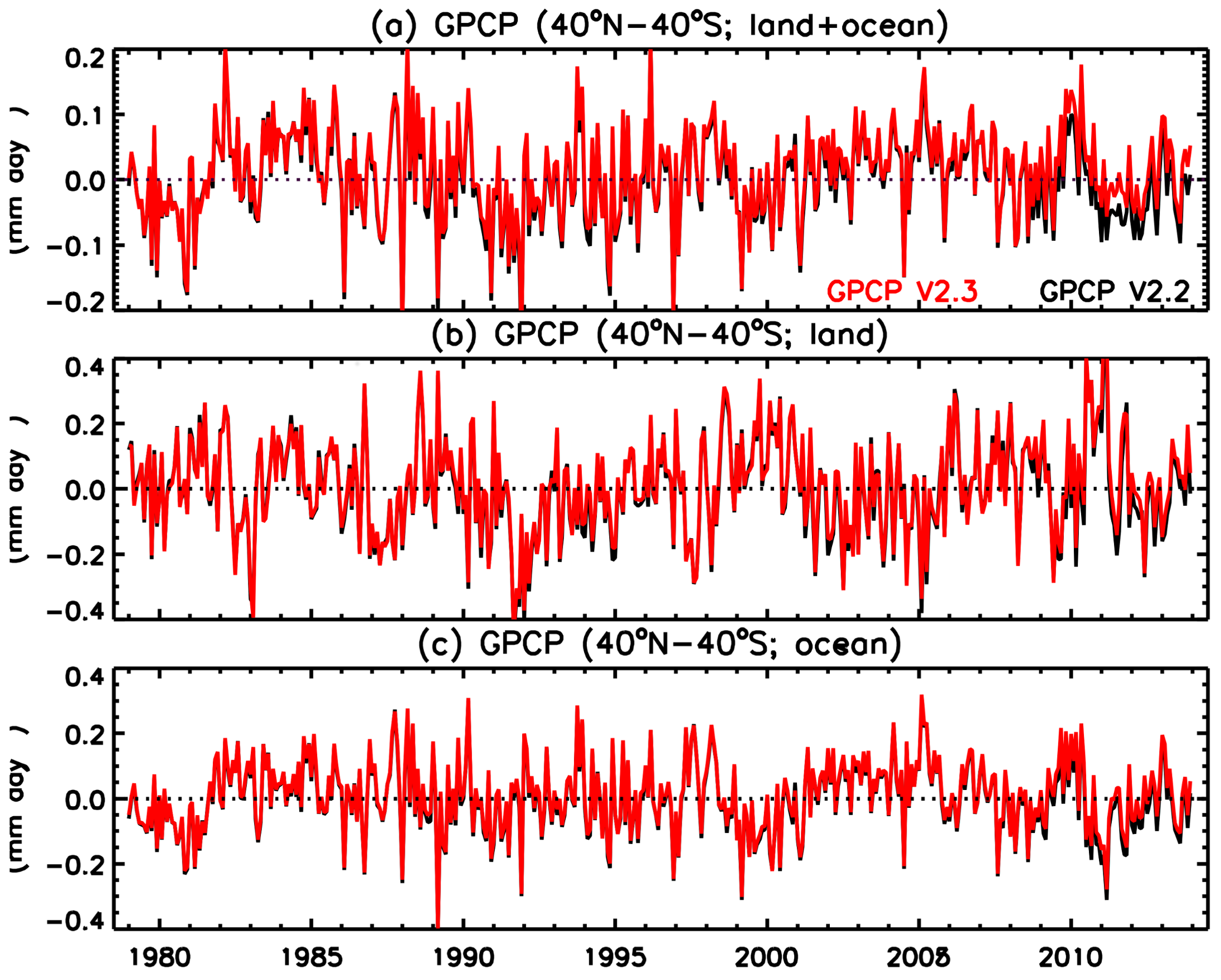
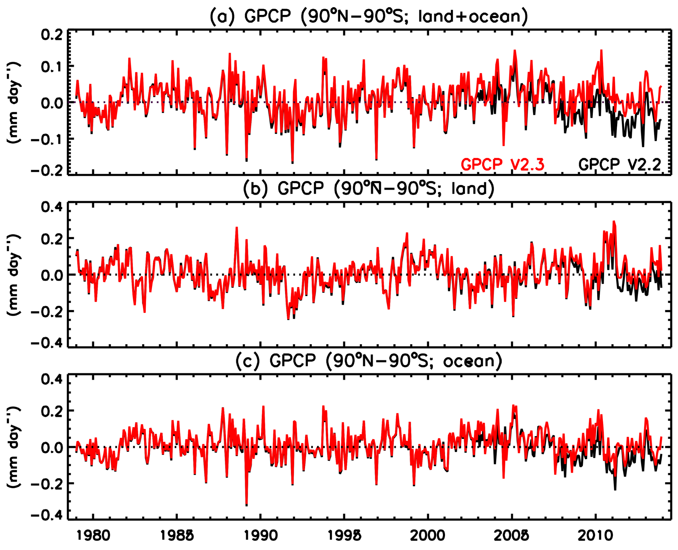
The changes described above make subtle but important corrections to the GPCP estimates, especially for 2003 and beyond. Figure 1 and Figure 2 respectively show the time histories of the global and tropical precipitation totals during the GPCP era for the two versions.

Table 1. Global mean precipitation (P, mm day⁻¹) from the Global Precipitation Climatology Project (GPCP) V2.3 and V2.2 and their differences from 1979–2013.

	Land + Ocean	Land	Ocean
V2.3	2.69	2.25	2.89
V2.2	2.68	2.23	2.88
V2.3–V2.2	0.01	0.02	0.01
Relative difference	+0.37%	+0.90%	+0.35%

,

Table 2. Global mean precipitation (P, mm day⁻¹) from GPCP V2.3 and V2.2 and their differences from 2003–2008 (TIROS Operational Vertical Sounder (TOVS) to Atmospheric Infrared Sounder (AIRS) transition is evident).

	Land + Ocean	Land	Ocean
V2.3	2.71	2.25	2.92
V2.2	2.69	2.24	2.90
V2.3-V2.2	0.02	0.01	0.02
Relative difference	+0.74%	+0.45%	+0.69%

,

Table 3. Global mean precipitation (P, mm day⁻¹) from GPCP V2.3 and V2.2 and their differences from 2009–2013 (both Special Sensor Microwave Imager (SSMI) to Special Sensor Microwave Imager/Sounder (SSMIS) and TOVS to AIRS transitions are evident).

	Land + Ocean	Land	Ocean
V2.3	2.70	2.27	2.89
V2.2	2.65	2.23	2.84
V2.3-V2.2	0.05	0.04	0.05
Relative difference	+1.89%	+1.79%	+1.76%

,

Table 4. Mean precipitation (P, mm day⁻¹) between 40° N and 40° S from GPCP V2.3 and V2.2 and their differences from 1979–2013.

	Land + Ocean	Land	Ocean
V2.3	2.95	2.81	3.00
V2.2	2.93	2.80	2.99
V2.3-V2.2	0.02	0.01	0.01
Relative difference	+0.68%	+0.36%	+0.33%

,

Table 5. Mean precipitation (P, mm day⁻¹) between 40° N and 40° S from GPCP V2.3 and V2.2 and their differences from 2003–2008.

	Land + Ocean	Land	Ocean
V2.3	2.97	2.81	3.03
V2.2	2.96	2.80	3.02
V2.3-V2.2	0.01	0.01	0.01
Relative difference	+0.34%	+0.36%	+0.33%

and

Table 6. Mean precipitation (P, mm day⁻¹) between 40° N and 40° S from GPCP V2.3 and V2.2 and their differences from 2009–2013.

	Land + Ocean	Land	Ocean
V2.3	2.96	2.84	3.00
V2.2	2.92	2.81	2.97
V2.3-V2.2	0.04	0.03	0.03
Relative difference	+1.37%	+1.07%	+1.01%

display the differences for the different intervals related to the changing satellite systems and for global means (Table 1, Table 2 and Table 3) and tropical means (40° N–40° S; Table 4, Table 5 and Table 6) for total, land, and ocean areas. Figure 1c and Figure 2c show the subtle shift upward over the last portion of the ocean data record (after 2003) from V2.2 to the new V2.3 due solely to the correction of the satellite inter-calibrations. The corrections in V2.3 affect ocean precipitation in two ways. From January 2009 onward, tropical ocean (40° N–40° S) precipitation increases in V2.3 by ~0.03 mm day⁻¹ (Table 6) due to the improved cross-calibration of estimates from SSMIS to those of the earlier SSMI estimates. From January 2003 onward, ocean precipitation estimates poleward of 40° N and 40° S increase slightly in V2.3, varying with latitude, up to ~0.04 mm day⁻¹ in the latitude band 40°–60° N due to the improved cross-calibration of precipitation estimates from TOVS to AIRS. This produces a slight change over global oceans (~0.01 mm day⁻¹) from 2003–2008 (Table 2) but a larger global ocean change (~0.05 mm day⁻¹) starting in 2009 (Table 3). Over land, the corrections are primarily due to the change from GPCC Monitoring to Full products for 2009 and later and a secondary increase due to the improved Full V7 GPCC product for the full period.

The corrections applied to obtain the GPCP V2.3 are all “small changes” (all less than 2%) but such changes are important when tracking trends on global and regional scales. Figure 1 and Figure 2 show the global and tropical totals as a function of time for the GPCP record and the effect of the corrections in V2.3 in the later years. The false decrease in global precipitation in V2.2 noted after ~2005 (Figure 1a) essentially disappears in V2.3 after the improvements and new data sets are incorporated. All these changes in magnitude are well within the bias error estimates for the GPCP climatology [15].

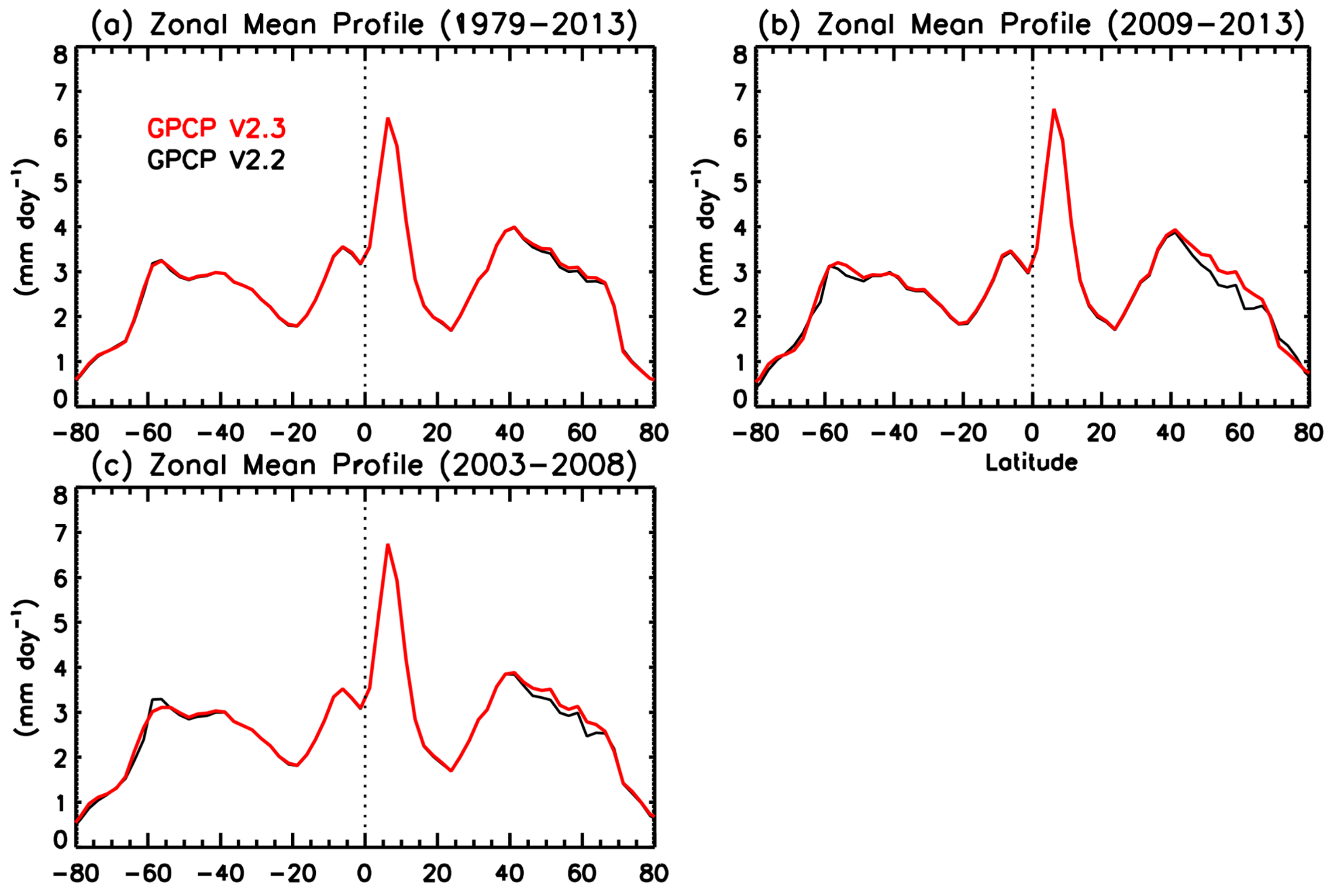
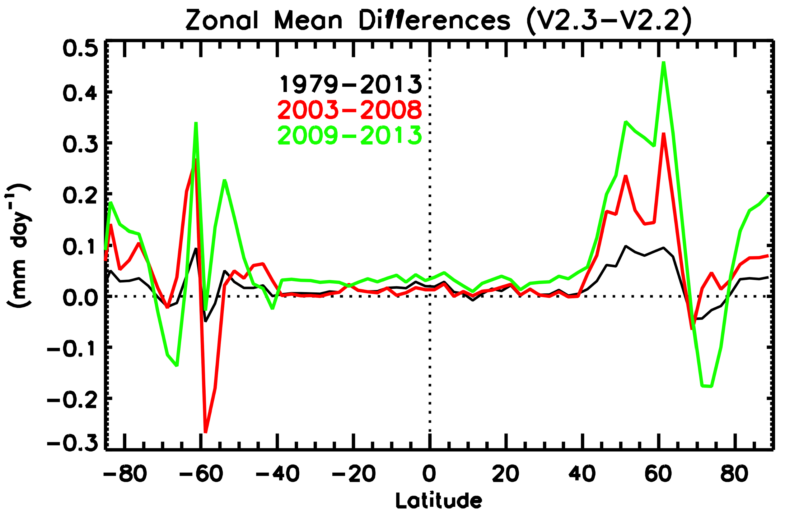
Figure 3 and Figure 4 focus on the zonal mean changes over the ocean. In Figure 3, the changes are only noticeable in the higher latitudes. Figure 4 shows the differences over oceans as a function of latitude; here one can see the small but noticeable increase in the tropics after 2009, and the latitudinal profile varying both positively and negatively, but overall positively, above 40° latitude. These variations are related to changes made in the weighting in the transition from SSMI/SSMIS-based estimates to AIRS-based estimates as a function of latitude above 40° latitude. Figure 5 shows difference maps for the same periods to further illustrate the regional differences. Over land, most of the changes are due primarily to the change to the GPCC V7 Full gauge analysis.

A detailed summary of climatological values, inter-annual variations, and trends using the GPCP V2.3 is given in [16], along with a summary of the comparisons with the recent precipitation estimates from the Tropical Rainfall Measuring Mission (TRMM) and CloudSat.

3. Monitoring Global Precipitation—A Quick Look at 2017

The GPCP Monthly data set (current Version 2.3) is typically produced approximately two-plus months after the month in question. An interim or preliminary GPCP analysis, called the Interim Climate Data Record (ICDR), is completed within ten days of the end of the month and allows for use in climate monitoring. The main differences are the use of the GPCC First Guess gauge precipitation analysis and less quality control than the GPCC Monitoring analysis. This quick availability of a monthly, globally complete precipitation analysis allows for nearly immediate (after 10 days) monitoring of precipitation for global and regional variations as compared to the long-term GPCP record and its climatology. When the final product is available two months later (under nominal availability of the input data sets), results can be updated. As an example of this “real-time” climate monitoring, a quick look at the just-completed year (2017) is described in this section.

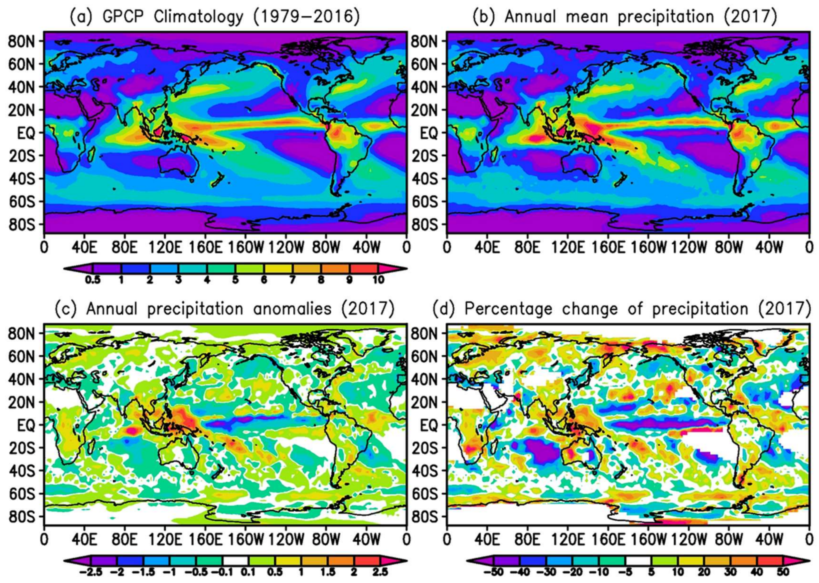
Figure 6 shows the GPCP climatology map (1979–2016), the annual mean map for 2017, and anomaly maps for 2017, for both rain rate magnitudes and percentages. The climatology map shows the usual maxima of the tropics and mid-latitudes with similar features, of course, for 2017 but with an obviously greater magnitude of mean rainfall over the Maritime Continent and surrounding areas. 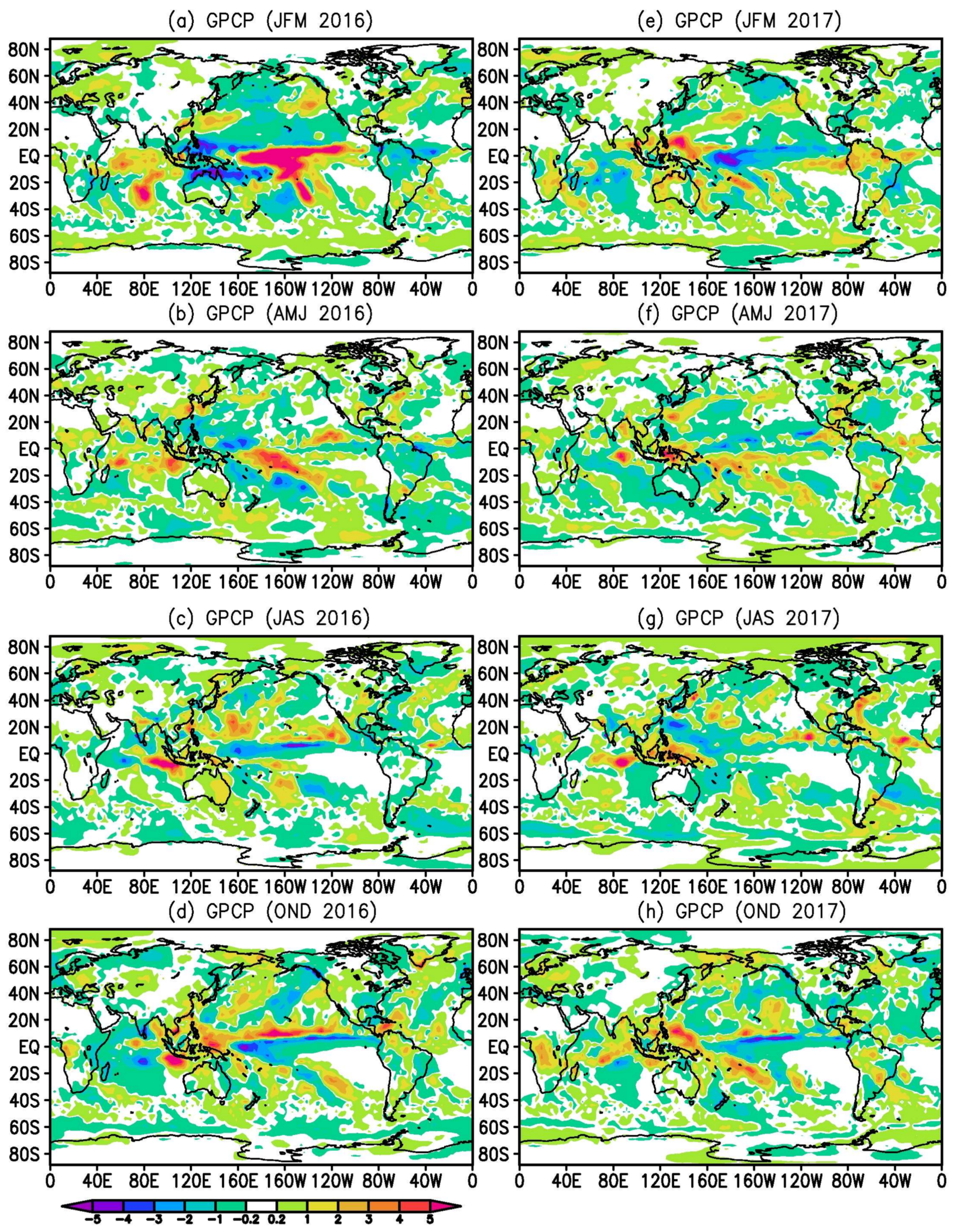The annual anomaly maps (Figure 6c,d) emphasize those features, showing a definite La Niña pattern with the strong positive anomaly over the western Pacific and a rainfall deficit over the central and eastern Pacific near the Equator. Indeed, the seasonal anomaly patterns during 2016 and 2017 (Figure 7) show a very strong El Niño pattern [17] in the tropics at the beginning of 2016 (Figure 7a) with a large positive maximum in the central Pacific Ocean and a rainfall deficit over the Maritime Continent. The ENSO pattern then evolves quickly to become a typical La Niña pattern by the end of 2016. The seasonal evolution during 2017 (Figure 7e–h) indicates that the La Niña features in the Pacific Ocean/Maritime Continent area existed in varying strengths during the entirety of 2017, resulting in the La Niña pattern across the Pacific for the year (seen in Figure 6c,d). Typical La Niña anomaly features can also be seen in some other locations, such as the positive feature in the tropical Atlantic, the negative anomaly off Baja, Mexico, extending into the southwest corner of the U.S., and a typical La Niña pattern along the east coast of Africa. A negative anomaly feature across the very southern tip of the African continent can be seen where Cape Town, South Africa, experienced its driest year since 1933 [18], possibly due in part to the La Niña. In Figure 6d, the Cape Town area is shown to have a spatially small but very strong negative percentage feature, emphasizing the connection between large-scale features and local impacts. Northern California, Oregon, and Washington in the northwestern corner of the U.S. (about 40° N, 120° W) show the strong positive anomaly related to heavy rain in the early part of the year. At higher latitudes, for example, across northern Eurasia and Alaska, positive anomalies dominate the inter-annual changes but also may be related to an estimated positive trend over the GPCP period in these areas.

Table 7. Global mean GPCP precipitation (mm day⁻¹) from 1979–2016 and in 2017. Also estimated are the annual anomalies in 2017 and corresponding percentage changes.

	Mean Rain Rate During 1979–2016 (mm day−1)	Mean Rain Rate in 2017 (mm day−1)	Annual Anomaly in 2017 (mm day−1)	Percentage Change in 2017 (%)
Land + Ocean	2.69	2.72	0.03	1.12
Land	2.24	2.34	0.10	4.46
Ocean	2.90	2.89	−0.01	−0.34

gives the estimated global mean rainfall rate for 2017 (2.72 mm/d) and the sub-totals for land and ocean. The global number is slightly (1%) higher than the 1979–2016 climatology with land areas contributing a value about 4% higher than the land climatology, related mainly to the year being dominated by the La Niña. For this exercise, the land precipitation values for years 2014–2017 from Version 2.3 have been adjusted upward by 2%. This adjustment is based on a difference in the version of gauge analysis that is used for the recent period (GPCC Monitoring) as compared to the pre-2014 era (GPCC Full Data Monthly). This is a small but significant adjustment and is based on an inter-comparison of the gauge analyses for an overlapping period. However, the results could change slightly when updated and, therefore, should be treated with caution.

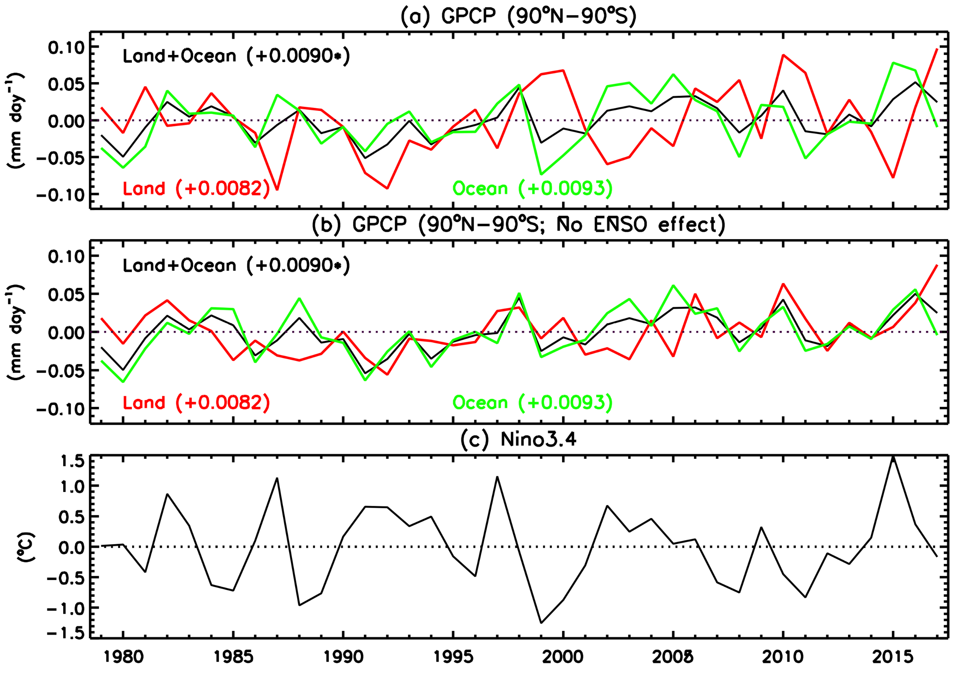
To put the global numbers for 2017 in context, Figure 8a shows plots of the annual anomaly of the global total (and ocean and land totals) from 1979 to 2017, with Figure 8c showing annual mean values for Niño 3.4 as a measure of ENSO for comparison with the annual anomaly values. The ocean and land values in Figure 8a “flip-flop” between El Niño and La Niña years, with the global total value having smaller year-to-year variations, although being larger during El Niño years (e.g., 1998, 2010, 2015–2016) [16]. The year 2017, a weak La Niña year, has an estimated record-setting high GPCP land value, compensated by a relatively low ocean value. The global value for 2017 is not a record high value, although the combination of 2016 and 2017 has an estimated mean that is higher than any other sequential two-year mean. The estimated trend is calculated for the three curves in Figure 8a and is slightly positive for all three, with a value of 0.009 mm day⁻¹ decade⁻¹ (0.33% per decade) for the global trend (significant at the 5% level). The trend values for both land and ocean are similar but are not significant due to the larger inter-annual variations. The second panel (Figure 8b) removes the ENSO effect on the annual anomalies using a regression technique and the Nino 3.4 index [19]. This results in reduced variations but the trend values stay the same and the significant results are also unchanged relative to the 5% threshold. The small, calculated global precipitation trend compared to the global surface temperature trend (0.16 K decade⁻¹) for the same period gives a 1.3% K⁻¹ for the rate of increase in global precipitation in relation to global warming. This value is close to the value often quoted coming from climate models but the GPCP-based value is very sensitive to the length (and homogeneity) of the record. As the length of the record for analyses such as GPCP increases, it is obvious that their value to the community will increase dramatically.

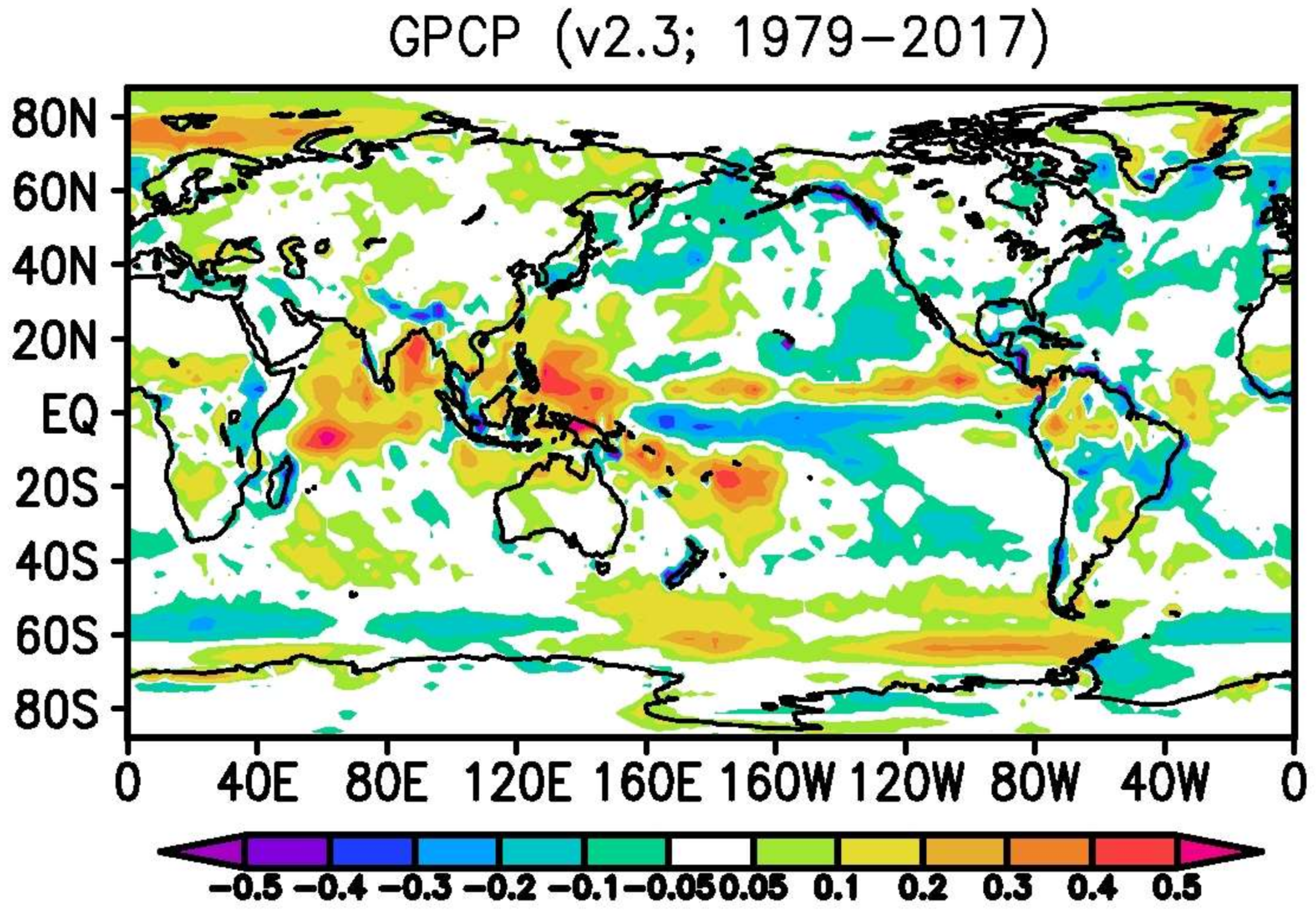
Although the global trends in Figure 8 are very small, the regional trends are larger and variable in the spatial domain (Figure 9) with the pattern showing an area of positive trend along most of the Inter-Tropical Convergence Zone (ITCZ), especially across the Pacific and Indian Oceans (see also [16]). Oceanic decreases north and south of the Pacific ITCZ are adjacent and weakly connected to decreases over land, including the southwestern U.S. A general scenario of “wet areas getting wetter, dry areas getting drier” is evident. At high northern latitudes, the positive trends noted across Eurasia and the Arctic Ocean to Alaska are similar to the positive anomaly features seen in Figure 6 for 2017. Adding one year (2017) to the data set does not significantly change the pattern in Figure 9, but also serves as a starting point for examining regional trends in relation to ENSO, inter-decadal variations, and global warming (see [16,20]).

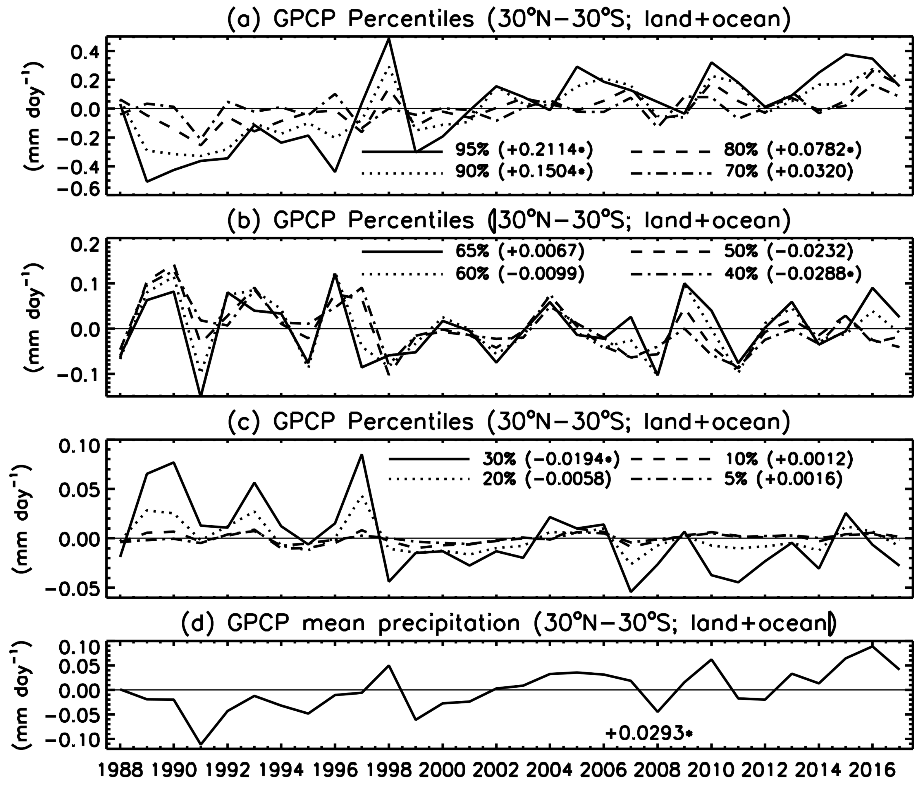
Data from 2017 have also been incorporated into the investigation of trends in rainfall intensity using the monthly GPCP analyses [21]. Focusing on the tropics and the post-1987 period (the satellite microwave era), percentiles (and other parameters related to intensity) at each grid box were computed and aggregated in the tropical latitude band (30° N–30° S) (see Figure 10). The mean tropical rainfall has a positive trend over the period (Figure 10d) but it is also evident that there are even stronger positive trends in the higher percentiles (increases in intense rainfall) with significant trends at percentiles greater than 70% (Figure 10a). At intermediate percentiles (30–40%), a downward trend is noted (Figure 10c). At low percentiles (not shown), trends were indeterminate but defined “dry areas” showed increases during the period. The year 2017 results helped solidify the trend results but an ENSO component is easily recognizable in the 95th percentile results with the El Niños of 1998, 2010, and 2016 (Figure 10b). There is also a decadal shift evident around 1998 related to the shift in the Pacific Decadal Oscillation (PDO).

4. Discussion and Conclusions

The GPCP Monthly analysis of global precipitation has been a widely used product in the scientific community for decades. The new version (Version 2.3) described in this paper has some small but significant changes, especially corrections and improvements for the years after 2002. Adjustments in the cross-calibration of rainfall estimates going from one satellite sensor type to another for two different sensor systems eliminated a slight, incorrect decrease in ocean precipitation in the earlier Version 2.2. The impact was small but perceptible in changes and trends of oceanic precipitation, especially when applied to large areas or the entire ocean, when the larger regional inter-annual variations often average out. The over-ocean change in magnitude from Version 2.2 to 2.3 is largest (1.8%) for the years after 2002 when the effects from the two different problems were present in V2.2. Over land areas, the new version of the GPCC gauge analysis also improved the merged analysis, leading to a small increase (1%) in climatological land precipitation. This is primarily due to the increased gauge sampling over the entire record and the update from the GPCC Monitoring product to the GPCC Full Data Monthly product for 2009–2013 (1.8% increase).

Although these corrections and adjustments are small, they are significant in accurately determining small variations (e.g., global inter-annual changes due to ENSO) or trends over large areas. The exercise in updating V2.2 to V2.3 is a good example of the necessary, continual effort to carefully homogenize and update input data sets and cross-calibrate over changes in satellite instruments or systems, and even conventional data analyses. This is especially true when dealing not just with a single instrument data set but also with a merged analysis of precipitation where a merger of various sources of information over both space and time is necessary to provide a globally complete analysis. The GPCP effort will continue to evolve with major improvements to the data set to include finer time and space resolutions, the use of modern algorithms, and the inclusion of information from recent satellite missions such as the Tropical Rainfall Measuring Mission (TRMM), the Global Precipitation Measurement (GPM) Mission, and CloudSat. Attention will also be focused on high latitude areas where current techniques and data need to be carefully evaluated and improved.

While some of the many research uses of the GPCP Monthly analysis have been described recently [16], routine monthly monitoring of global precipitation can now be accomplished with the GPCP ICDR product. The review of the 2017 global precipitation in this paper is an example of how to use the GPCP data to understand how it fits in with the GPCP history and climatology. The general La Niña pattern for 2017 and the evolution from the early 2016 El Niño pattern is clearly indicated in the tropics and the analysis allows for monitoring of teleconnections across the globe. The past year (2017) has the typical positive global land anomaly for a La Niña year and fits into the ocean–land ENSO flip-flop seen for most of the GPCP period. The 2017 global total (land plus ocean) is one of the highest for the 1979–2017 period, outdone by only 2016 and 1998 (both El Niño years). The upward trend in global precipitation is significant at the 5% level with a calculated 1.3%/K trend when compared to the surface temperature trend over the period. One year does not significantly affect trends but since the precipitation trend map is certainly non-uniform, the annual anomaly map does contain some anomalies due to trends, although these are still relatively small. However, the examination of precipitation intensity shows significant trends in the tropics using the Monthly data, with increases of more intense rainfall (in terms of percentile) and a decrease of intermediate intensity values. The year 2017 results fit into those scenarios with the intense rain having a positive anomaly and the intermediate intensity rain having a negative anomaly, as compared to the climatological values.

The routine calculation of the Interim product shortly after the month in question allows for the use of this research data set for examination and monitoring of inter-annual variations and even trends in means and intensities in real time (in a climate sense). This routine monitoring with GPCP appears to be worthwhile and will likely be continued and expanded by the GPCP group and others.