Statistical Analysis of Spatiotemporal Heterogeneity of the Distribution of Air Quality and Dominant Air Pollutants and the Effect Factors in Qingdao Urban Zones

 ,
, 
Abstract
:1. Introduction
2. Study Area, Materials, and Methodology
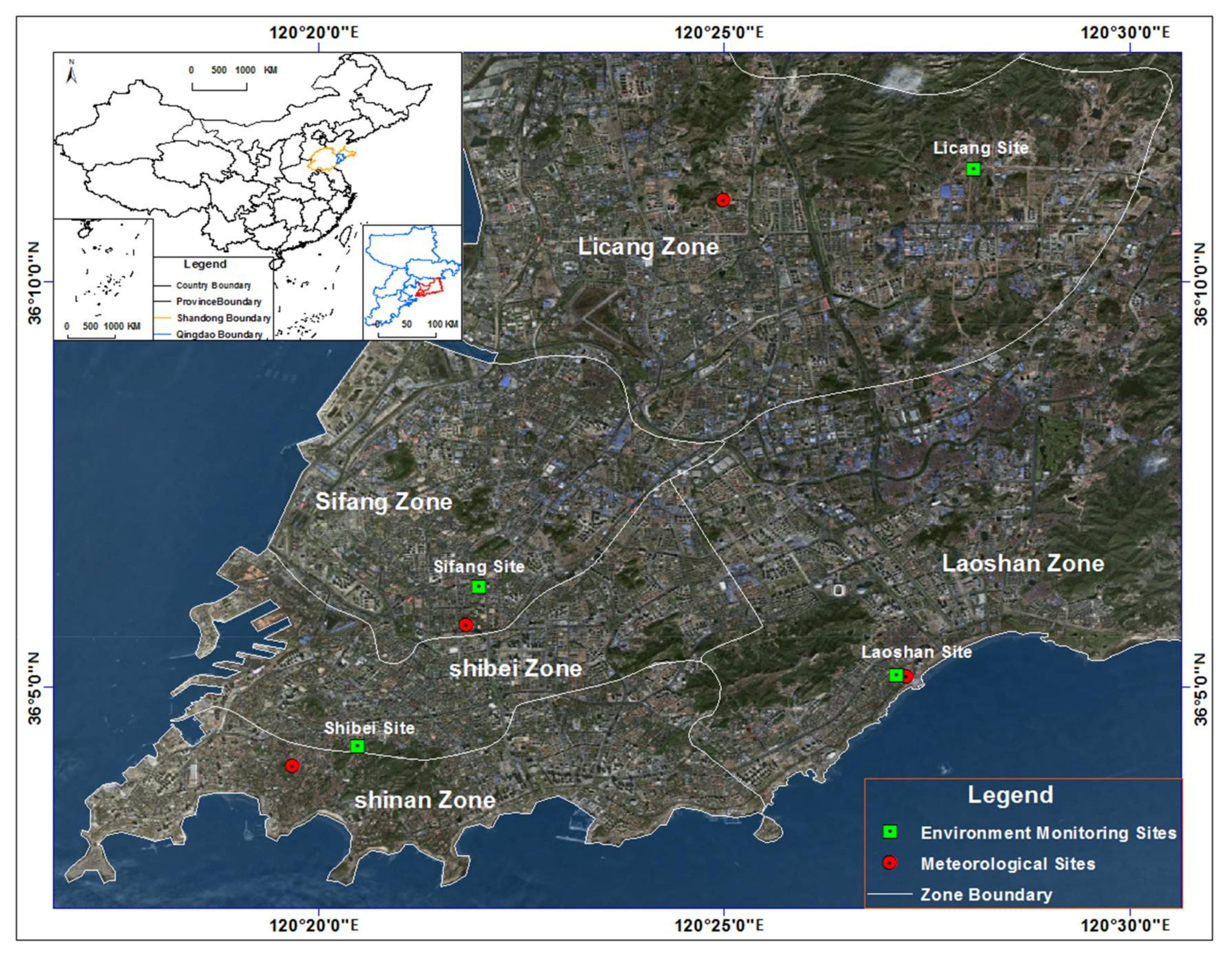
2.1. Study Area
2.2. Materials
2.3. Methodology
2.3.1. Spatiotemporal Heterogeneity Analysis Methods
2.3.2. Effect Factors Analysis Methods
3. Results
3.1. Spatiotemporal Heterogeneity of AQ Distribution
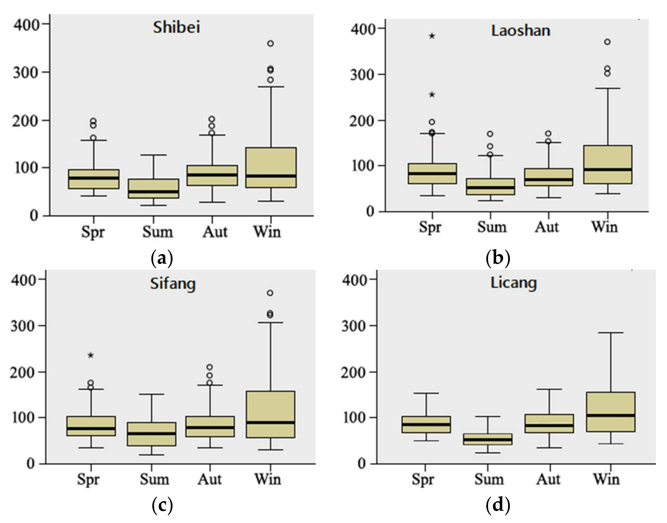
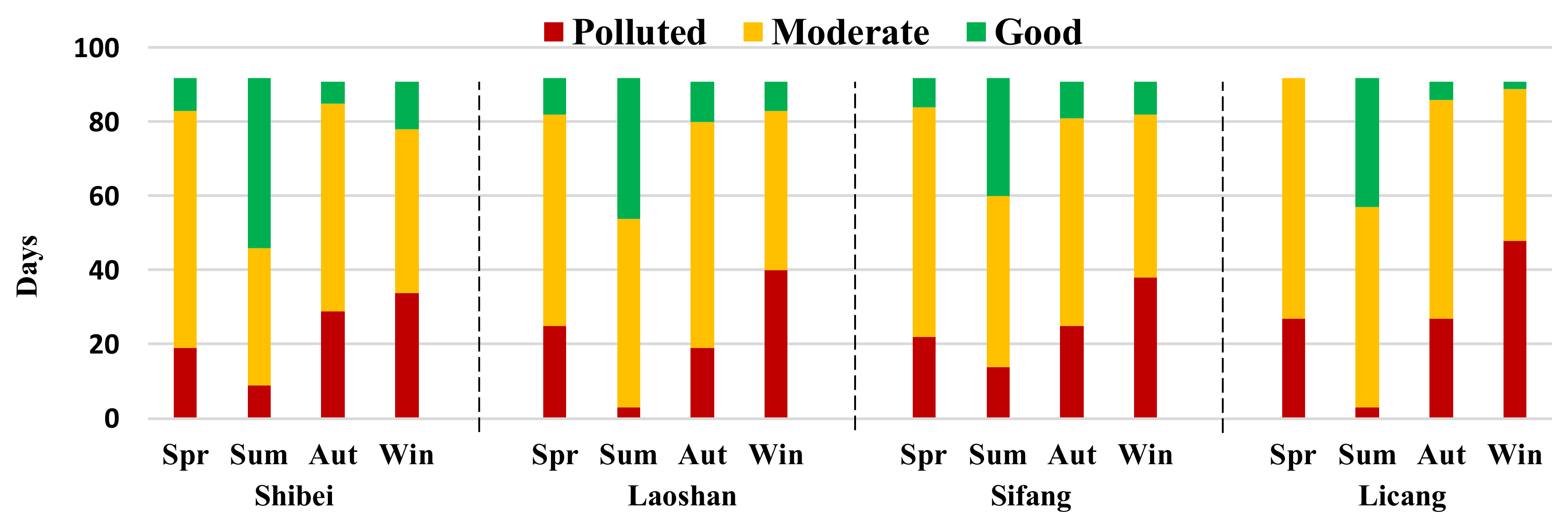
3.1.1. Temporal Heterogeneity of AQ Distribution
3.1.2. Spatial Heterogeneity of AQ Distribution
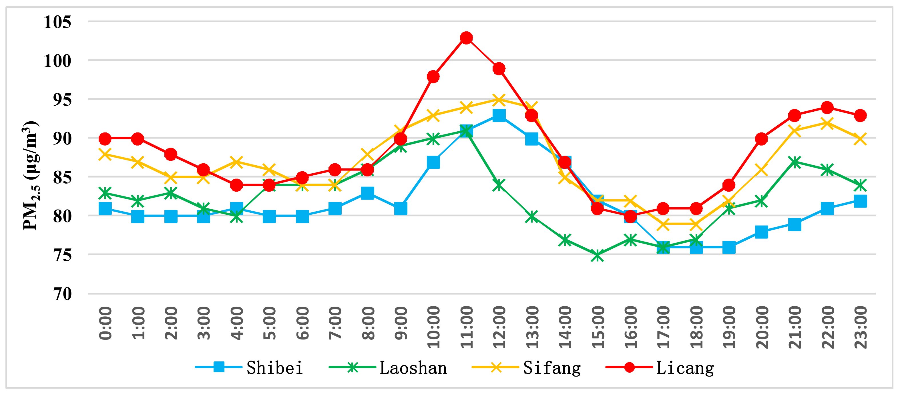
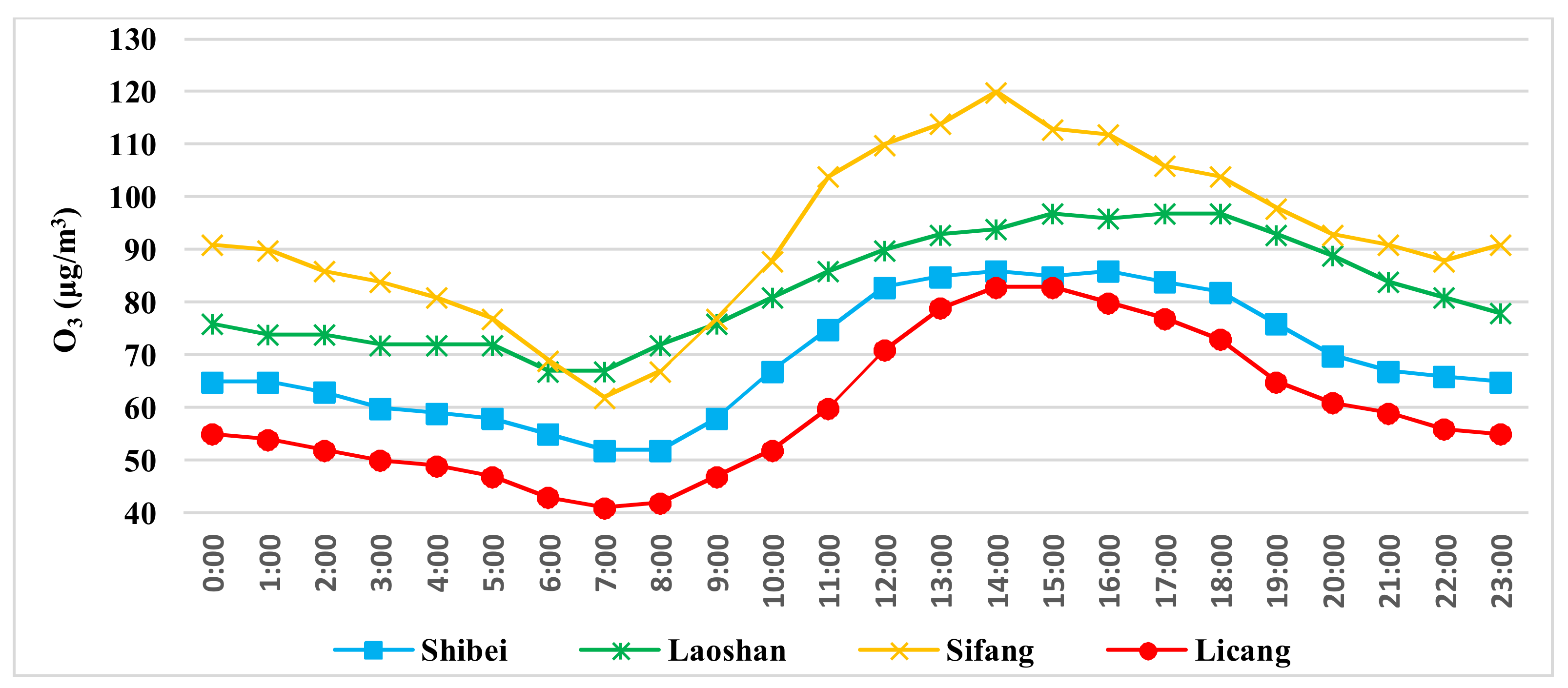
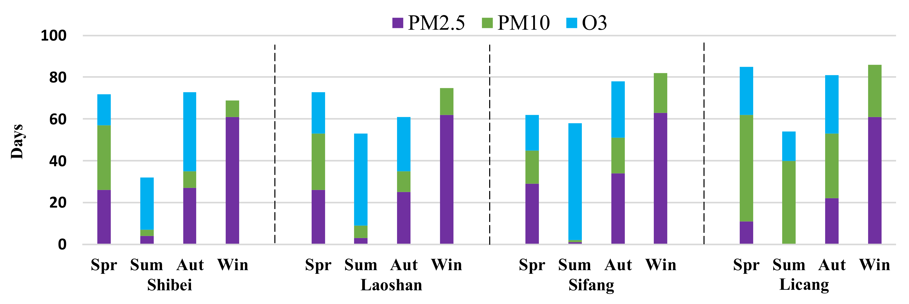
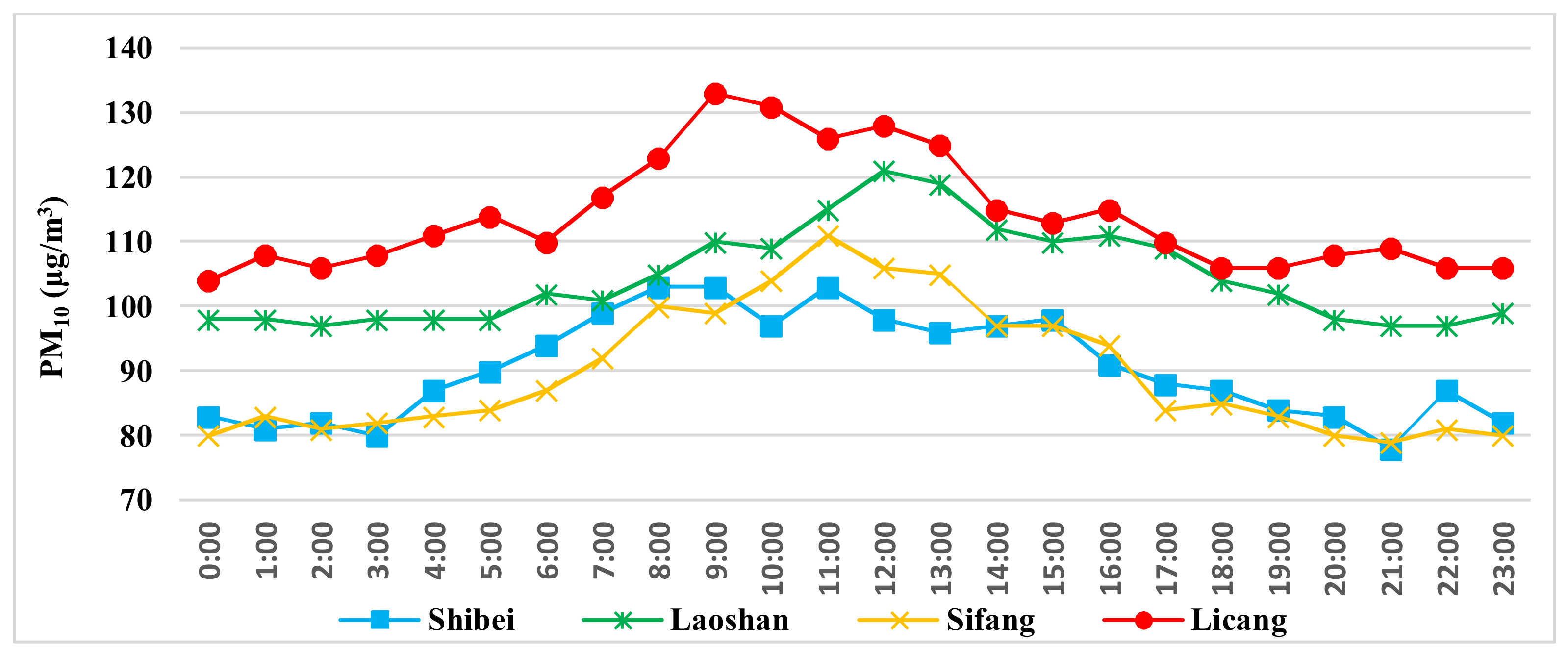
3.2. Spatiotemporal Heterogeneity of Dominant Air Pollutants Distribution
3.3. The Effect of the Relevant Factors on the Dominant Air Pollutants
4. Discussion
4.1. Temporal Heterogeneity of AQ and Dominant Air Pollutants
4.2. Spatial Heterogeneity of AQ and Dominant Air Pollutants
5. Conclusions
Acknowledgments
Author Contributions
Conflicts of Interest
References
- Unal, Y.S.; Toros, H.; Deniz, A.; Incecik, S. Influence of meteorological factors and emission sources on spatial and temporal variations of PM10 concentrations in Istanbul metropolitan area. Atmos. Environ. 2011, 45, 5504–5513. [Google Scholar] [CrossRef]
- Watson, L.; Lacressonnière, G.; Gauss, M.; Engardt, M.; Andersson, C.; Josse, B.; Marécal, V.; Nyiri, A.; Sobolowski, S.; Siour, G.; et al. The impact of meteorological forcings on gas phase air pollutants over Europe. Atmos. Environ. 2015, 119, 240–257. [Google Scholar] [CrossRef]
- Gualtieri, G.; Toscano, P.; Crisci, A.; Di Lonardo, S.; Tartaglia, M.; Vagnoli, C.; Zaldei, A.; Gioli, B. Influence of road traffic, residential heating and meteorological conditions on PM10 concentrations during air pollution critical episodes. Environ. Sci. Pollut. Res. Int. 2015, 22, 19027–19038. [Google Scholar] [CrossRef] [PubMed]
- Zhang, H.N.; Wang, Y.H.; Park, T.W.; Deng, Y. Quantifying the relationship between extreme air pollution events and extreme weather events. Atmos. Res. 2017, 188, 64–79. [Google Scholar] [CrossRef]
- Wang, G.L.; Xue, J.J.; Zhang, J.Z. Analysis of Spatial-temporal Distribution Characteristics and Main Cause of Air Pollution in Beijing-Tianjin-Hebei Region in 2014. Meteorol. Environ. Sci. 2016, 39, 34–42, (In Chinese with English Abstract). [Google Scholar]
- Bao, C.Z.; Chai, P.F.; Lin, H.B.; Zhang, Z.Y.; Ye, Z.H.; Gu, M.J.; Lu, H.C.; Shen, P.; Jin, M.J.; Wang, J.B.; et al. Association of PM2.5 pollution with the pattern of human activity: A case study of a developed city in Eastern China. Atmos. Environ. 2016, 66, 1202–1213. [Google Scholar] [CrossRef] [PubMed]
- Ma, X.Y.; Jia, H.L. Particulate matter and gaseous pollution in three megacities over China: Situation and implication. Atmos. Environ. 2016, 140, 476–494. [Google Scholar] [CrossRef]
- Wei, Y.G.; Gu, J.; Wang, H.W.; Yao, T.; Wu, Z.Z. Uncovering the culprits of air pollution: Evidence from China’s economic sectors and regional heterogeneities. J. Clean. Prod. 2018, 171, 1481–1493. [Google Scholar] [CrossRef]
- Kahn, J.; Yardley, J. As China Roars, Pollution Reaches Deadly Extremes. The New York Times, 26 August 2007. [Google Scholar]
- Lopez, R.; Galinato, G.I.; Fiscal, A.I. spending and the environment: Theory and empirics. J. Environ. Econ. Manag. 2011, 62, 180–198. [Google Scholar] [CrossRef]
- Dong, Q.L.; Wang, Y.; Li, P.Z. Multifractal behavior of an air pollutant time series and the relevance to the predictability. Environ. Pollut. 2017, 222, 444–457. [Google Scholar] [CrossRef] [PubMed]
- Xie, Y.Y.; Zhao, B.; Zhang, L.; Luo, R. Spatiotemporal variations of PM2.5 and PM10 concentrations between 31 Chinese cities and their relationships with SO2, NO2, CO and O3. Particuology 2015, 20, 141–149. [Google Scholar] [CrossRef]
- Wang, H.J.; Chen, H.P. Understanding the recent trend of haze pollution in eastern China: Roles of climate change. Atmos. Chem. Phys. 2016, 16, 4205–4211. [Google Scholar] [CrossRef]
- Wang, Z.B.; Fang, C.L. Spatial-temporal characteristics and determinants of PM2.5 in the Bohai Rim Urban Agglomeration. Chemosphere 2016, 148, 148–162. [Google Scholar] [CrossRef] [PubMed]
- Li, L.Y.; Yan, D.Y.; Xu, S.H.; Huang, M.L.; Wang, X.X.; Xie, S.D. Characteristics and source distribution of air pollution in winter in Qingdao, eastern China. Environ. Pollut. 2017, 224, 44–53. [Google Scholar] [CrossRef] [PubMed]
- Li, Q.; Wang, E.R.; Zhang, T.T.; Hu, H. Spatial and Temporal Patterns of Air Pollution in Chinese Cities. Water Air Soil Pollut. 2017, 228, 92. [Google Scholar] [CrossRef]
- Chen, Y.; Xie, S.; Luo, B.; Zhai, C. Characteristics and origins of carbon aceousaerosol in the Sichuan Basin, China. Atmos. Environ. 2014, 94, 215–223. [Google Scholar] [CrossRef]
- Zhang, C.; Ni, Z.W.; Ni, L.P. Multifractal detrended cross-correlation analysis between PM2.5 and meteorological factors. Physica A 2015, 438, 114–123. [Google Scholar] [CrossRef]
- Cheng, J.H.; Dai, S.; Ye, X.Y. Spatiotemporal heterogeneity of industrial pollution in China. China Econ. Rev. 2016, 40, 179–191. [Google Scholar] [CrossRef]
- Li, L.; Qian, J.; Ou, C.Q.; Zhou, Y.X.; Guo, C.; Guo, Y. Spatial and temporal analysis of Air Pollution Index and its timescale-dependent relationship with meteorological factors in Guangzhou, China, 2001–2011. Environ. Pollut. 2014, 190, 75–81. [Google Scholar] [CrossRef] [PubMed]
- Pan, L.; Yao, E.J.; Yang, Y. Impact analysis of traffic-related air pollution based on real-time traffic and basic meteorological information. J. Environ. Manag. 2015, 183, 510–520. [Google Scholar] [CrossRef] [PubMed]
- Yan, S.J.; Cao, H.; Chen, Y.; Wu, C.Z.; Hong, T.; Fan, H.L. Spatial and temporal characteristics of air quality and air pollutants in 2013 in Beijing. J. Environ. Manag. 2016, 23, 13996–14007. [Google Scholar] [CrossRef] [PubMed]
- Zhang, Z.Y.; Zhang, X.L.; Gong, D.Y.; Quan, W.J.; Zhao, X.J.; Ma, Z.Q.; Kim, S.J. Evolution of surface O3 and PM2.5 concentrations and their relationships with meteorological conditions over the last decade in Beijing. Atmos. Environ. 2015, 108, 67–75. [Google Scholar] [CrossRef]
- Shen, C.H.; Li, C.L.; Si, Y.L. A detrended cross-correlation analysis of meteorological and API data in Nanjing, China. Physica A 2015, 419, 417–428. [Google Scholar] [CrossRef]
- Huang, F.F.; Li, X.; Wang, C. PM2.5 Spatiotemporal Variations and the Relationship with Meteorological Factors during 2013–2014 in Beijing, China. PLoS ONE 2015, 10, e0141642. [Google Scholar] [CrossRef] [PubMed]
- Escobedo, F.J.; Nowak, D.J. Spatial heterogeneity and air pollution removal by an urban forest. Landsc. Urban Plan. 2009, 90, 102–110. [Google Scholar] [CrossRef]
- He, C.F.; Huang, Z.J.; Ye, X.Y. Spatial heterogeneity of economic development and industrial pollution in urban China. Stoch. Environ. Res. Risk Assess. 2014, 28, 767–781. [Google Scholar] [CrossRef]
- Nami, P.; Jahanbakhsh, P.; Fathalipour, A. The Role and Heterogeneity of Visual Pollution on the Quality of Urban Landscape Using GIS; Case Study: Historical Garden in City of Maraqeh. Open J. Geol. 2016, 6, 20–29. [Google Scholar] [CrossRef]
- Wen, W.; Cheng, S.Y.; Chen, X.F.; Wang, G.; Li, S.; Wang, X.; Liu, X.Y. Impact of emission control on PM2.5 and the chemical composition change in Beijing-Tianjin-Hebei during the APEC summit 2014, China. Environ. Sci. Pollut. Res. 2016, 23, 4509–4521. [Google Scholar] [CrossRef] [PubMed]
- Li, Y.; Chen, Q.L.; Zhao, H.J.; Wang, L.; Tao, R. Variations in PM10, PM2.5 and PM1.0 in an Urban Area of the Sichuan Basin and Their Relation to Meteorological Factors. Atmosphere 2015, 6, 150–163. [Google Scholar] [CrossRef]
- Hu, J.L.; Wang, Y.G.; Ying, Q.; Zhang, H.L. Spatial and temporal variability of PM2.5 and PM10 over the North China Plain and the Yangtze River Delta, China. Atmos. Environ. 2014, 95, 598–609. [Google Scholar] [CrossRef]
- Wang, Y.G.; Ying, Q.; Hu, J.L.; Zhang, H.L. Spatial and temporal variations of six criteria air pollutants in 31 provincial capital cities in China during 2013–2014. Environ. Int. 2014, 73, 413–422. [Google Scholar] [CrossRef] [PubMed]
- Li, R.; Cui, L.L.; Li, J.L.; Zhao, A.; Fu, H.B.; Wu, Y.; Zhang, L.W.; Kong, L.D.; Chen, J.M. Spatial and temporal variation of particulate matter and gaseous pollutants in China during 2014–2016. Atmos. Environ. 2017, 161, 235–246. [Google Scholar] [CrossRef]
- Tian, G.J.; Qiao, Z.; Xu, X.L. Characteristics of particulate matter (PM10) and its relationship with meteorological factors during 2001-2012 in Beijing. Environ. Pollut. 2014, 192, 266–274. [Google Scholar] [CrossRef] [PubMed]
- Batterman, S.; Xu, L.Z.; Chen, F.; Chen, F.; Zhong, X.F. Characteristics of PM2.5 concentrations across Beijing during 2013–2015. Atmos. Environ. 2016, 145, 104–114. [Google Scholar] [CrossRef] [PubMed]
- Lu, H.; Wang, S.S.; Li, Y.; Gong, H.; Han, J.Y.; Wu, Z.L.; Yao, S.L.; Zhang, X.M.; Tang, X.J.; Jiang, B.Q. Seasonal variations and source apportionment of atmospheric PM2.5-bound polycyclic aromatic hydrocarbons in a mixed multi-function area of Hangzhou, China. Environ. Sci. Pollut. Res. 2017, 24, 16195–16205. [Google Scholar] [CrossRef] [PubMed]
- Zheng, S.; Zhou, X.Y.; Singh, R.P.; Wu, Y.Z.; Ye, Y.M.; Wu, C.F. The Spatiotemporal Distribution of Air Pollutants and Their Relationship with Land-Use Patterns in Hangzhou City, China. Atmosphere 2017, 8, 110. [Google Scholar] [CrossRef]
- Cui, H.Y.; Chen, W.H.; Dai, W.; Liu, H.; Wang, X.M.; He, K.B. Source apportionment of PM2.5 in Guangzhou combining observation data analysis and chemical transport model simulation. Atmos. Environ. 2015, 116, 262–271. [Google Scholar] [CrossRef]
- Yang, Y.; Christakos, G. Spatiotemporal Characterization of Ambient PM2.5 Concentrations in Shandong Province (China). Environ. Sci. Technol. 2015, 49, 13431–13438. [Google Scholar] [CrossRef] [PubMed]
- Xu, W.Y.; Zhao, C.S.; Ran, L.; Deng, Z.Z.; Liu, P.F.; Ma, N.; Lin, W.L.; Xu, X.B.; Yan, P.; He, X.; et al. Characteristics of pollutants and their correlation to meteorological conditions at a suburban site in the North China Plain. Atmos. Chem. Phys. 2011, 11, 4353–4369. [Google Scholar] [CrossRef]
- Ge, B.Z.; Wang, Z.F.; Lin, W.L.; Xu, X.B.; Li, J.; Ji, D.S.; Ma, Z.Q. Air pollution over the North China Plain and its implication of regional transport: A new sight from the observed evidences. Environ. Pollut. 2018, 234, 29–38. [Google Scholar] [CrossRef] [PubMed]
- Wu, R.D.; Zhou, X.H.; Wang, L.P.; Wang, Z.; Zhou, Y.; Zhang, J.Z.; Wang, W.X. PM2.5 Characteristics in Qingdao and across Coastal Cities in China. Atmosphere 2016, 8, 77. [Google Scholar] [CrossRef]
- Chen, D.S.; Wang, X.T.; Nelson, P.; Li, Y.; Zhao, N.; Zhao, Y.H.; Lang, J.L.; Zhou, Y.; Guo, X.R. Ship emission inventory and its impact on the PM2.5 air pollution in Qingdao Port, North China. Atmos. Environ. 2017, 166, 351–361. [Google Scholar] [CrossRef]
- Cong, X.C.; Qu, J.H.; Yang, G.S. On-road measurements of pollutant concentration profiles inside Yangkou tunnel, Qingdao, China. Environ. Geochem. Health 2016, 39, 1179–1190. [Google Scholar] [CrossRef] [PubMed]
- Chinese Ministry of Environmental Protection. Technical Regulation on Ambient Air Quality Index; HJ633-2102; Chinese Ministry of Environmental Protection: Beijing, China, February 2012.
- Vargha, A.; Delaney, H.D. The Kruskal-Wallis test and stochastic homogeneity. J. Educ. Behav. Stat. 1998, 23, 170–192. [Google Scholar] [CrossRef]
- Ruxton, G.D.; Beauchamp, G. Some suggestions about appropriate use of the Kruskal–Wallis test. Anim. Behav. 2008, 76, 1083–1087. [Google Scholar] [CrossRef]
- Ostertagova, E.; Ostertag, O.; Kovac, J. Methodology and Application of the Kruskal-Wallis Test. Appl. Mech. Mater. 2014, 611, 115–120. [Google Scholar] [CrossRef]
- Zimmerman, D.W. An efficient alternative to the Wilcoxon signed-ranks test for paired nonnormal data. J. Gen. Psychol. 1996, 123, 29. [Google Scholar] [CrossRef]
- Taheri, S.M.; Hesamian, G. A generalization of the Wilcoxon signed-rank test and its applications. Stat. Pap. 2013, 54, 457–470. [Google Scholar] [CrossRef]
- Yeo, I.K. An algorithm for computing the exact distribution of the Wilcoxon signed-rank statistic. J. Korean Stat. Soc. 2017, 46, 328–338. [Google Scholar] [CrossRef]
- Fredricks, G.A.; Nelsen, R.B. On the relationship between Spearman’s rho and Kendall’s tau for pairs of continuous random variables. J. Stat. Plan. Inference 2007, 137, 2143–2150. [Google Scholar] [CrossRef]
- Genest, C.; Rémillard, B.; Beaudoin, D. Goodness-of-fit tests for copulas: A review and a power study. Insurance 2009, 44, 199–213. [Google Scholar] [CrossRef]
- Staudt, A. Tail risk, systemic risk and Copulas. Casualty Actuar. Soc. Forum 2010, 2, 1–20. [Google Scholar]
- Pourkhanali, A.; Kim, J.M.; Tafakori, L. Measuring systemic risk using vine–copula. Econ. Model. 2016, 53, 63–74. [Google Scholar] [CrossRef]
- Zhao, X.W.; Gao, Q.; Yue, Y.J.; Duan, L.; Pan, S. A System Analysis on Steppe Sustainability and Its Driving Forces—A Case Study in China. Sustainability 2018, 10, 233. [Google Scholar] [CrossRef]
- Forbes, K.J.; Rigobon, R. No contagion, only interdependence: Measuring stock market comovements. J. Financ. 2002, 57, 2223–2261. [Google Scholar] [CrossRef]
- Salvadori, G.; Michele, C.D. On the Use of Copulas in Hydrology: Theory and Practice. J. Hydrol. Eng. 2007, 12, 369–380. [Google Scholar] [CrossRef]
- Kouchak, A.; Bardossy, A.; Habib, E. Conditional simulation of remotely sensed rainfall data using a non–Gaussian v–transformed copula. Adv. Water Resour. 2010, 33, 624–634. [Google Scholar] [CrossRef]
- Musafer, G.N.; Thompson, M.H.; Kozan, E. Copula–based spatial modelling of geometallurgical variables. In Proceedings of the Second AUSIMM International Geometallurgy Conference, Brisbane, Australia, 30 September–2 October 2013; pp. 239–246. [Google Scholar]
- Klein, B.; Meissner, D.; Lisniak, D. Predictive Uncertainty Estimation of Hydrological Multi–Model Ensembles Using Pair–Copula Construction. Water 2016, 8, 125. [Google Scholar] [CrossRef]
- Atalay, F.; Tercan, A.E. Coal resource estimation using Gaussian copula. Int. J. Coal Geol. 2017, 175, 1–9. [Google Scholar] [CrossRef]
- Kumar, A.; Goyal, P. Forecasting of air quality in Delhi using principal component regression technique. Atmos. Pollut. Res. 2011, 2, 436–444. [Google Scholar] [CrossRef]
- Huang, R.; Guo, L.N.; Ma, Y.; Yu, S.B. Relationship between air quality and meteorological conditions from 2006 to 2012 in Qingdao. J. Meteorol. Environ. 2015, 31, 37–43, (In Chinese with English Abstract). [Google Scholar]
- Tang, G.; Wang, Y.; Li, X.; Ji, D.; Hsu, S.; Gao, X. Spatial-temporal variations in surface ozone in Northern China as observed during 2009–2010 and possible implications for future air quality control strategies. Atmos. Chem. Phys. 2012, 12, 2757–2776. [Google Scholar] [CrossRef]
- Liu, J.; Zhang, X.L.; Xu, X.F.; Xu, H.H. Comparison analysis of variation characteristics of SO2, NOx, O3 and PM2.5 between rural and urban areas, Beijing. Environmentalscienc 2008, 29, 1059–1065. [Google Scholar] [CrossRef]
- Chen, Y.C.; Zang, L.; Chen, J.Y.; Xu, D.; Yao, D.F.; Zhao, M.R. Characteristics of ambient ozone (O3) pollution and health risks in Zhejiang Province. Environ. Sci Pollut. Res. 2017, 24, 27436–27444. [Google Scholar] [CrossRef] [PubMed]
- Cheng, H.R.; Guo, H.; Wang, X.M.; Saunders, S.M.; Lam, S.H.M.; Jiang, F.; Wang, T.J.; Ding, A.J.; Lee, S.C.; Ho, K.F. On the relationship between ozone and its precursors in the Pearl River Delta: application of an observation-based model (OBM). Environ. Sci. Pollut. Res. 2010, 17, 547–560. [Google Scholar] [CrossRef] [PubMed]
- Wu, Y.S.; Zhang, F.Y.; Shi, Y.; Pilot, E.; Lin, L.Y.; Fu, Y.B.; Krafft, T.; Wang, W.Y. Spatiotemporal characteristics and health effects of air pollutants in Shenzhen. Atmos. Pollut. Res. 2015, 7, 58–65. [Google Scholar] [CrossRef]
- Shen, Z.X.; Cao, J.J.; Zhang, L.M.; Liu, L.; Zhang, Q.; Li, J.J.; Han, Y.M.; Zhu, C.S.; Zhao, Z.Z.; Liu, S.X. Day-night differences and seasonal variations of chemical species in PM10 over Xi’an, northwest China. Environ. Sci. Pollut. Res. 2014, 21, 3697–3705. [Google Scholar] [CrossRef] [PubMed]
- Xu, L.L.; Chen, X.Q.; Chen, J.S.; Zhang, F.W.; He, C.; Du, K.; Wang, Y. Characterization of PM10 atmospheric aerosol at urban and urban background sites in Fuzhou city, China. Environ. Sci. Pollut. Res. 2012, 19, 1443–1453. [Google Scholar] [CrossRef] [PubMed]
- Liu, Z.R.; Hu, B.; Wang, L.L.; Wu, F.K.; Gao, W.K.; Wang, Y.S. Seasonal and diel variation in particulate matter (PM10 and PM2.5) at an urban site of Beijing: Analyses from a 9-year study. Environ. Sci. Pollut. Res. 2015, 22, 627–642. [Google Scholar] [CrossRef] [PubMed]


| Zones | Population (million) | Residential Area (km2) | Greening Rate | Key Enterprises | Prevailing Wind Direction | |||
|---|---|---|---|---|---|---|---|---|
| Spring | Summer | Autumn | Winter | |||||
| Shibei | 0.5846 | 10.0647 | 28.50% | 1 | S | S | N-W | N-W |
| Laoshan | 0.4844 | - | 49.13% | 0 | S-E/E-S | E-S | N-W | N-E |
| Sifang | 0.4275 | 8.5226 | 27.89% | 1 | S-E | S-E | N-W/W-N | W-N |
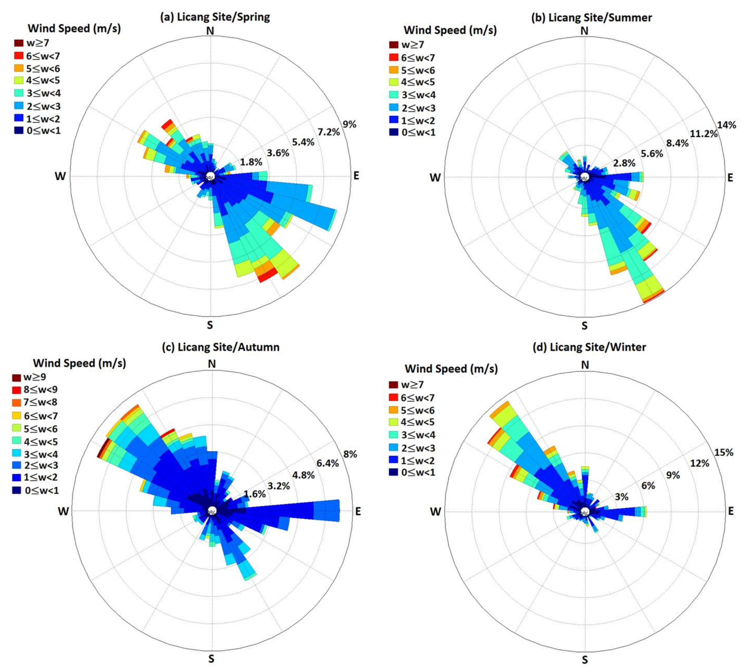
| Licang | 0.5414 | 15.7445 | 41.71% | 2 | S-E | S-E | W-N/N-W | N-W/W-N |
| Statistical Variable | Environment Monitoring Sites | ||||
|---|---|---|---|---|---|
| Shibei | Laoshan | Sifang | Licang | ||
| Mean of AQI | 85 | 85 | 89 | 90 | |
| Standard Deviation of AQI | 48.13 | 49.49 | 50.16 | 50.63 | |
| Days of AQ levels | Good | 74 | 67 | 59 | 42 |
| Moderate | 201 | 212 | 208 | 219 | |
| Polluted | 91 | 87 | 99 | 105 | |
| Pairs of Sites | p Value | H0 |
|---|---|---|
| Laoshan ↔ Licang | <0.001 | Reject |
| Laoshan ↔ Shibei | 0.238 | Accept |
| Laoshan ↔ Sifang | 0.001 | Reject |
| Licang ↔ Sifang | <0.001 | Reject |
| Licang ↔ Shibei | <0.001 | Reject |
| Shibei ↔ Sifang | <0.001 | Reject |
| Statistical Variable | Environment Monitoring Sites | ||||
|---|---|---|---|---|---|
| Shibei | Laoshan | Sifang | Licang | ||
| Days of dominant pollutants | PM10 | 50 | 56 | 53 | 148 |
| PM2.5 | 118 | 116 | 127 | 94 | |
| O3 | 78 | 90 | 100 | 65 | |
| Pairs of Sites | PM10 in Spring | O3 in Summer | PM2.5 in Winter | |||
|---|---|---|---|---|---|---|
| p Value | H0 | p Value | H0 | p Value | H0 | |
| Laoshan ↔ Licang | <0.001 | Reject | <0.001 | Reject | <0.001 | Reject |
| Laoshan ↔ Shibei | <0.001 | Reject | <0.001 | Reject | 0.248 | Accept |
| Laoshan ↔ Sifang | <0.001 | Reject | <0.001 | Reject | <0.001 | Reject |
| Licang ↔ Sifang | <0.001 | Reject | <0.001 | Reject | 0.01 | Reject |
| Licang ↔ Shibei | <0.001 | Reject | <0.001 | Reject | <0.001 | Reject |
| Shibei ↔ Sifang | 0.410 | Accept | <0.001 | Reject | <0.001 | Reject |
| Shibei | Laoshan | Sifang | Licang | |||||||||
|---|---|---|---|---|---|---|---|---|---|---|---|---|
| PM10 | O3 | PM2.5 | PM10 | O3 | PM2.5 | PM10 | O3 | PM2.5 | PM10 | O3 | PM2.5 | |
| SO2 | 0.538 | −0.209 | 0.844 | 0.458 | 0.286 | 0.554 | 0.340 | 0.350 | 0.796 | 0.420 | 0.700 | 0.588 |
| NO2 | 0.439 | −0.334 | 0.758 | 0.062 | −0.039 | 0.719 | −0.295 | 0.388 | 0.480 | 0.103 | −0.284 | 0.645 |
| CO | 0.556 | 0.206 | 0.854 | 0.392 | 0.397 | 0.761 | 0.471 | 0.589 | 0.738 | 0.376 | 0.354 | 0.657 |
| Temp 1 | 0.232 | 0.641 | −0.331 | 0.496 | 0.298 | −0.339 | 0.262 | 0.630 | −0.247 | 0.388 | 0.496 | −0.290 |
| Press 2 | −0.345 | −0.525 | 0.239 | - 5 | - | - | −0.260 | −0.126 | 0.179 | −0.221 | −0.394 | 0.186 |
| WindS 3 | 0.07 | −0.100 | −0.094 | 0.524 | 0.196 | 0.077 | 0.029 | 0.009 | 0.078 | 0.333 | 0.415 | −0.050 |
| Humid 4 | −0.282 | −0.658 | −0.081 | - | - | - | −0.230 | −0.552 | 0.102 | −0.445 | −0.307 | −0.094 |
© 2018 by the authors. Licensee MDPI, Basel, Switzerland. This article is an open access article distributed under the terms and conditions of the Creative Commons Attribution (CC BY) license (http://creativecommons.org/licenses/by/4.0/).
Share and Cite
Zhao, X.; Gao, Q.; Sun, M.; Xue, Y.; Ma, R.; Xiao, X.; Ai, B. Statistical Analysis of Spatiotemporal Heterogeneity of the Distribution of Air Quality and Dominant Air Pollutants and the Effect Factors in Qingdao Urban Zones. Atmosphere 2018, 9, 135. https://doi.org/10.3390/atmos9040135
Zhao X, Gao Q, Sun M, Xue Y, Ma R, Xiao X, Ai B. Statistical Analysis of Spatiotemporal Heterogeneity of the Distribution of Air Quality and Dominant Air Pollutants and the Effect Factors in Qingdao Urban Zones. Atmosphere. 2018; 9(4):135. https://doi.org/10.3390/atmos9040135
Chicago/Turabian StyleZhao, Xiangwei, Qian Gao, Meng Sun, Yunchuan Xue, RuiJin Ma, Xingyuan Xiao, and Bo Ai. 2018. "Statistical Analysis of Spatiotemporal Heterogeneity of the Distribution of Air Quality and Dominant Air Pollutants and the Effect Factors in Qingdao Urban Zones" Atmosphere 9, no. 4: 135. https://doi.org/10.3390/atmos9040135
APA StyleZhao, X., Gao, Q., Sun, M., Xue, Y., Ma, R., Xiao, X., & Ai, B. (2018). Statistical Analysis of Spatiotemporal Heterogeneity of the Distribution of Air Quality and Dominant Air Pollutants and the Effect Factors in Qingdao Urban Zones. Atmosphere, 9(4), 135. https://doi.org/10.3390/atmos9040135