Land-Use Regression Modelling of Intra-Urban Air Pollution Variation in China: Current Status and Future Needs

Abstract

Rapid urbanization in China is leading to substantial adverse air quality issues, particularly for NO₂ and particulate matter (PM). Land-use regression (LUR) models are now being applied to simulate pollutant concentrations with high spatial resolution in Chinese urban areas. However, Chinese urban areas differ from those in Europe and North America, for example in respect of population density, urban morphology and pollutant emissions densities, so it is timely to assess current LUR studies in China to highlight current challenges and identify future needs. Details of twenty-four recent LUR models for NO₂ and PM_2.5/PM₁₀ (particles with aerodynamic diameters <2.5 µm and <10 µm) are tabulated and reviewed as the basis for discussion in this paper. We highlight that LUR modelling in China is currently constrained by a scarcity of input data, especially air pollution monitoring data. There is an urgent need for accessible archives of quality-assured measurement data and for higher spatial resolution proxy data for urban emissions, particularly in respect of traffic-related variables. The rapidly evolving nature of the Chinese urban landscape makes maintaining up-to-date land-use and urban morphology datasets a challenge. We also highlight the importance for Chinese LUR models to be subject to appropriate validation statistics. Integration of LUR with portable monitor data, remote sensing, and dispersion modelling has the potential to enhance derivation of urban pollution maps.

1. Introduction

Air quality in China has suffered as a consequence of rapid economic growth and urbanization. In 2016, 81%, 62%, 46%, 38%, 4.1% and 1.4% of 74 main cities in China (including provincial capitals and prefectural and municipality-level cities) failed the Chinese air quality standards that are listed in

Table 1. Chinese air quality standards for concentrations of SO₂, NO₂, CO, O₃, PM₁₀, and PM_2.5 [10]. Also shown for comparison are the World Health Organization (WHO) air quality guidelines, where they exist [11].

Pollutant	Grade a	Annual Mean (µg/m3)	24-h Mean (µg/m3)	1-h Mean (µg/m3)
SO2	I	20	50	150
	II	60	150	500
	WHO		20	500 b
NO2	I	40	80	200
	II	40	80	200
	WHO	40		200
CO c	I		4	10
	II		4	10
O3	I		100 d	160
	II		160 d	200
	WHO		100 d
PM10	I	40	50
	II	70	150
	WHO	20	50
PM2.5	I	15	35
	II	35	75
	WHO	10	25

^a Grade I applies to special regions such as national parks; Grade II applies to all other areas, including urban and industrial areas. ^b 10-min mean. ^c The units for CO concentration are mg/m³. ^d Daily maximum 8-h mean.

for PM_2.5, PM₁₀, NO₂, O₃, CO and SO₂, respectively [1]. (PM_2.5 and PM₁₀ refer to the mass concentration of particulate matter with aerodynamic diameters less than 2.5 µm and less than 10 µm, respectively.) Furthermore, while the Chinese air quality standard for NO₂ is the same as the World Health Organization (WHO) air quality guideline, those for PM_2.5, PM₁₀, and O₃ are currently less stringent than the WHO equivalents (Table 1). The air quality problem is particularly serious in regions of rapid population growth such as Beijing, Shanghai, the Pearl River Delta (PRD) (Pearl River Delta refers to cities that cover nine prefectures of Guangdong province (Guangzhou, Shenzhen, Zhuhai, Dongguan, Zhongshan, Foshan, Huizhou, Jiangmen, and Zhaoqing), Hong Kong, and Macau), and their surrounding areas [2]. Ample evidence that air pollution leads to adverse health effects and economic losses, including recent studies in China [3,4,5,6,7,8,9], underscores the need to quantify human exposure to air pollution in China in order to determine health impacts and monitor the effectiveness of mitigation policies.

Since 2013, the China National Environmental Monitoring Center (CNEMC) has been implementing a nationwide monitoring network for the routine measurement of ambient air pollutant concentrations. However, the monitoring network only provides concentrations at a limited number of discrete points—for example, the 22 monitoring stations covering a 50 km × 50 km area over Beijing equates to an average of 113 km² per station [12]—which is inadequate to describe the spatial variability of urban air pollution. The misclassification of human exposure can lead to a loss of power in epidemiological studies and the attenuation of health risk estimates [13].

A popular approach in Europe and North America for deriving intra-urban estimates of air pollutant concentrations is land-use regression (LUR) modelling. LUR is a stochastic technique that regresses spatially-explicit predictor variables (e.g., land cover, traffic, topography) onto monitored pollutant concentrations within a geographic information system [14,15]. The relationship enables prediction of pollutant concentrations at unmonitored locations. Selection of potential predictor variables uses a priori knowledge that they may contribute to, or influence, emissions and concentrations of modelled pollutants. Examples of input data commonly needed for a LUR model are shown in

Table 2. Summary of example input data for the application of a land-use regression (LUR) model.

Input	Detailed Components
pollutant data	regularity monitoring data
	purpose-designed campaign
land-use classification	residential land
	industrial land
	urban green space
	street morphology (aspect ratio)
traffic data	road network by road classification
	numbers and types of vehicles
	railways
census data	population density
	household density
meteorology	wind field
	temperature
topography	altitude
	slope angle
emission data	emission inventory
remote sensing data	satellite data

.

The expansion of the CNMEC (and other) monitoring networks is driving a growing number of LUR studies in China. As the nature of urban areas in China differ from those in Europe and North America, as outlined in Section 2, it is timely to assess the present status of LUR modelling in China in the context of identifying what lessons can be learned to advance this field from the similarities and differences with LUR studies applied elsewhere. The objectives of this paper are therefore: (i) to briefly summarize differences between Chinese urban areas and those in Europe and North America in the context of LUR modelling of air pollution concentrations; (ii) to summarize the state-of-the-art of LUR air pollution modelling in China; and (iii) to highlight the current gaps in LUR modelling in China in comparison with LUR models in Europe and North America and make recommendations on future needs for China. The majority of applications of LUR have been for NO₂ and PM_2.5/PM₁₀, since these pollutants are a priority for regulatory monitoring and interventions due to their public health effects. This paper therefore focuses on LUR studies for NO₂ and PM_2.5/PM₁₀ only. Twenty-four such studies in China were identified from the peer-reviewed English-language literature and their details are used as the basis for discussion in this paper.

2. Differences between Urban Areas in China and in Europe and North America

2.1. Pace of Urbanization

China’s rapid economic development has led to extremely rapid urban population growth. At the end of 2011, China’s urban population exceeded that of rural dwellers for the first time [16,17] and the trend is continuing—the proportion of urban population in China is expected to reach approximately 70% by 2025 [18]. The extent of built-up area in China has expanded correspondingly rapidly. The growth rate of built-up land from 2000 to 2010 was 2.14 times higher than in the previous decade [19]. Between 2010 and 2016 the area of land undergoing urban construction increased from 39,760 km² to 52,750 km² and possession of private vehicles increased from 59.4 to 163.3 million [20].

2.2. Magnitude and Density of Urbanization

Urban areas in China are characterized by populations of several million [21], with considerably higher population densities than the vast majority of urban areas in Europe and North America. The average urban population density in China across all built-up areas with a population >500,000 is 5100 per km², compared with equivalent values of 2900 per km² for the European Union (3100 per km² for all of Europe including Russia) and 1600 per km² for North America (1200 and 2500 per km² for the USA and Canada individually) [22].

2.3. Air Pollutant Emissions

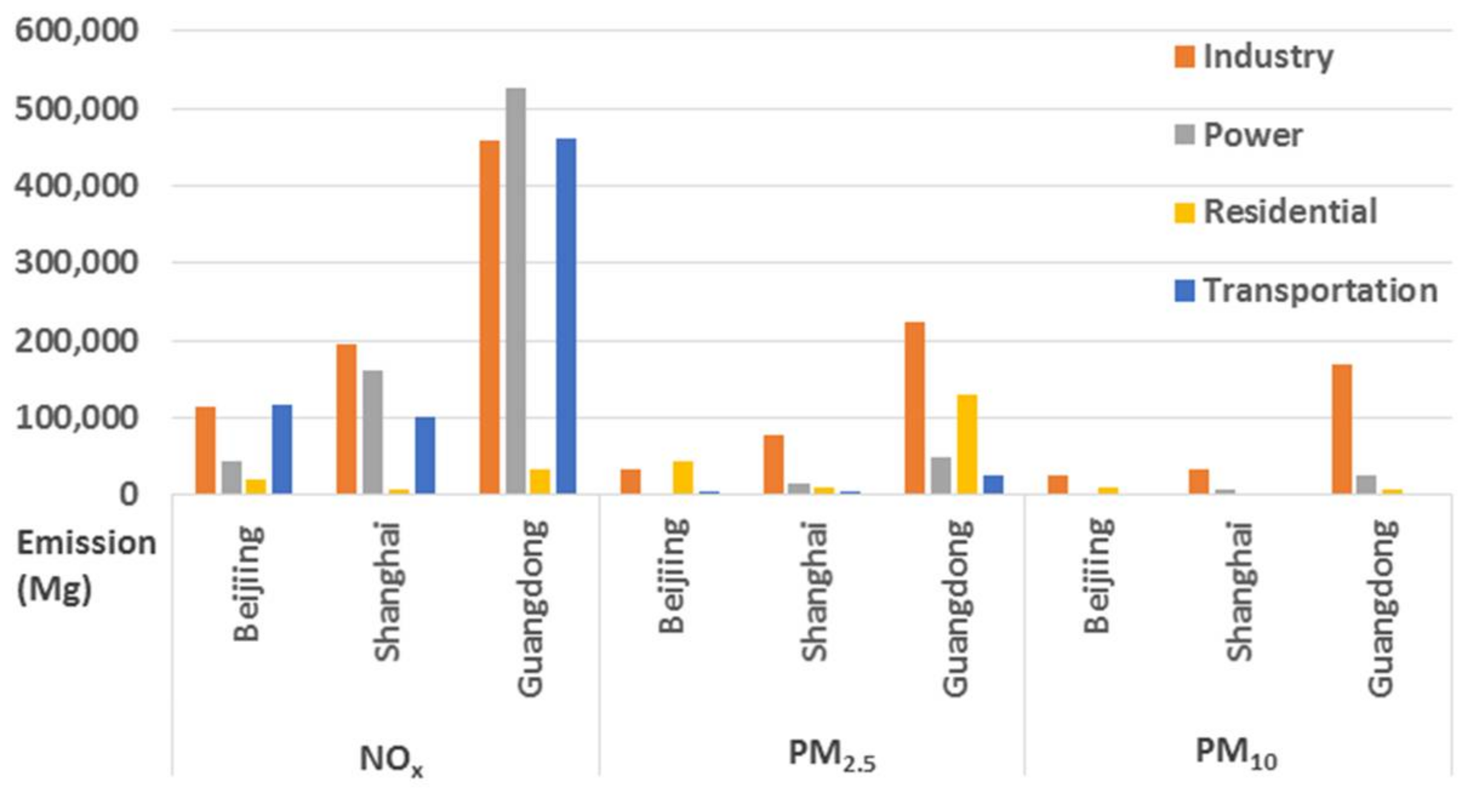
Greater population density leads to increased emissions of air pollutants in a given area. The sectorial contributions to NO_x (sum of NO and NO₂), PM_2.5 and PM₁₀ emissions presented in Figure 1 for three illustrative urban areas (Beijing, Shanghai, and Guangdong province) show that power generation, industry and transportation all contribute substantially to NO_x emissions. Industrial sources dominate the contributions to emissions of PM, although residential combustion (heating and cooking) also contributes substantially to emissions of fine PM (PM_2.5).

Greater emissions density in China can also derive from a lag in implementation [23] and/or in compliance [24] with industrial and vehicle emissions standards compared with that in Europe and North America. Poorer fuel quality has also been reported as contributing to greater per vehicle emissions in China [25].

2.4. Urban Topography

The higher urban population density in China is a consequence of the greater proportion of multi-story residential and commercial buildings. In 2016, China completed the most high-rise buildings (84) with heights exceeding 200 m of any country in the world. It was the ninth year in a row that China topped this list. Thirty-one cities in China had at least one 200-m-plus building completion in 2016 [27]. The greater urban ‘roughness’ and extent of street canyons impact the dispersion of air pollutants both directly and indirectly via differential changes in surface albedo and surface temperatures.

3. LUR Models for Chinese Urban Areas

Twenty-four LUR studies were identified from Web of Science and Google Scholar, using the following search phrases and keywords: land use regression; LUR; China; Hong Kong; Taiwan; air pollution; NO₂; PM_2.5; PM₁₀. A first search was undertaken on 11 November 2017, with a follow-up search for any new literature on 3 February 2018. Language was limited to English but there was no restriction on publication date. Characteristics of these studies are summarized in

Table 3. Characteristics of recent air pollution land-use regression studies in China that include NO₂ or PM_2.5/PM₁₀ as a modelled pollutant.

Reference	Study Area	Area (km2)	Population (million)	Type of Sites Used	No. of Monitoring Sites	Pollutants	Sampling Period 1	Predictor Variables Collected
Yang et al., 2017 [41]	PRD	56,000	57.6	regulatory monitoring sites	69	NO2, PM2.5	01/12/2013 to 30/11/2014	geographic character, land use type, traffic indicator, urbanization indicator, wind field, satellite remote sensing, air quality model
Wu et al., 2017 [45]	Taipei Metropolitan area	2327	6.6	regulatory monitoring sites	17	PM2.5	2006 to 2012	annual average of SO2 and NOx, land use type, land mark, road network, Normalized Difference Vegetation Index (NDVI)
Shi et al., 2017 [38]	Hong Kong	1100	>7	regulatory monitoring sites	15	CO, NO2, NOx, O3, SO2, PM2.5, PM10	2011 to 2015	traffic network/volume, urban land use, population density, geo-location and physical geography of monitoring points, wind availability
Lee et al., 2017 [34]	Hong Kong	1104	7.24	sampling campaign	43, 97, 63, 84	NO, NO2, PM2.5, BC	24/04/2014 to 30/05/2014, 18/11/2014 to 06/10/2015	annual average traffic density, road length, traffic loading, urban build-up, land use, point feature, value extracted at point, distance
Huang et al., 2017 [43]	Nanjing	6596	8.27	regulatory monitoring sites	9	PM2.5, SO2, NO2, O3	01/01/2013 to 31/12/2013	industrial emission, population density, topography, meteorological variables, road network, land use
Chen et al., 2017 [50]	Tianjin	11,760	>12	regulatory monitoring sites	28	PM2.5	2014	population, land use, road network, distance to coast
Anand and Monks, 2017 [51]	Hong Kong	1104	7.35	regulatory monitoring sites	11	NO2	2005 to 2015	vehicle emissions, industrial emissions, residential emissions, dry deposition, ocean deposition, surface elevation, surface temperature, wind advection, location
Xu et al., 2016 [52]	Wuhan	8494	>10	regulatory monitoring sites	9	SO2, NO2, PM10	2007 to 2014	land use, socio-economic development, energy use, road density, industry emission, meteorological condition
Shi et al., 2016 [37]	Hong Kong	1104	7.35	mobile	222	PM2.5, PM10	14 days May to September 2015	traffic and transport, land use, physical geography, population, urban/building morphology
Meng et al., 2016 [53]	Shanghai	6300	23	regulatory monitoring sites	28	PM10	2008	land use, road network, emission, population
Liu et al., 2016 [54]	Shanghai	6341	23.8	regulatory monitoring sites	53	PM2.5, NO2	2014	land use, road networks, distance to the ocean, longitude and latitude, distance to major air pollution sources, suburban and urban area
Hu et al., 2016 [55]	Beijing	16,411	21.69	regulatory monitoring sites	35	PM2.5	2014	land use, terrain, transportation, population, polluting enterprises, points of interest, distance to the city center, buildings, natural landscape
Gong et al., 2016 [56]	Liaoning Province	145,900	42.21	regulatory monitoring sites	34	SO2, NO2, PM10	2013	canyon indicator, elevation, normalized difference vegetative index, distance to air pollutant point source emissions, road density, population density, Gross Domestic Product
Wu et al., 2015 [40]	Beijing	16,411	21.69	regulatory monitoring sites	35	PM2.5	04/03/2013 to 05/03/2014	road length, land cover, population density, catering services, bus stop density, intersection density, others
Meng et al., 2015 [57]	Shanghai	6300	23	regulatory monitoring sites	38	NO2	2008–2011	population, road network, land use, industrial emissions, coastline
Liu et al., 2015 [36]	Changsha	1917	7	sampling campaign (regulatory monitoring sites)	74 (9), 36 (9)	NO2, PM10	14 days in each season of 2010	road network, land use, meteorology
Li et al., 2015 [35]	Changsha	1917	7	sampling campaign	80, 40	NO2, PM10	14 days in each season	road length, land use, green space, water area
Ho et al., 2015 [32]	Taipei Metropolitan area	2327	6.5	sampling campaign	25	PM2.5, Si, S, Ti, Mn, Fe, Ni, Cu, Zn	01/2010 to 10/2010	land use, road network, floor level, population
Wu et al., 2014 [44]	Kaohsiung City	2952	2.27	sampling campaign	29	PM2.5, Si, S, Ti, Mn, Fe, Ni, Cu, Zn	03/2011 to 12/2011	land use, road network, sampling height, population
Lee et al., 2014 [33]	Taipei Metropolitan area	786	6.5	sampling campaign	40	NOx, NO2	10/2009 to 09 2010	road length, land use, population and household density, altitude
Chen et al., 2012 [58]	Tianjin	11,920	>10	regulatory monitoring sites	30	SO2, NO2, PM10	2006	road network, traffic volume, land use, population density, meteorology, physical variables, pollution sources
Yu et al., 2011 [59]	Taipei	271.8	2.7	regulatory monitoring sites	18	PM2.5	2005 to 2007	land use, road network
Chen et al., 2010b [39]	Jinan	8177	60.485		14	SO2, NO2, PM10	01/08/2008 to 31/07/2009	traffic, land use, population density, physical condition, meteorological condition, others
Chen et al., 2010a [60]	Tianjin	11,920	>10	regulatory monitoring sites	30	NO2, PM10	heating season: 15/11/2006 to 15/03/2006; non heating: 16/03/2006 to 14/11/2006	major roads, land use, population, meteorological variables and distance to sea

¹ The form of the dates are DD/MM/YYYY and MM/YYYY.

. LUR models for NO₂ and/or PM_2.5/PM₁₀ have been developed for individual Chinese cities (Hong Kong, Nanjing, Tianjing, Shanghai, Beijing, Changsha, Wuhan, Jinan, and Kaohsing) and regions (PRD, Taipei Metropolitan area, and Liaoning Province). The recent dates of the publications demonstrate the recent impetus for LUR modelling in China.

3.1. Monitoring Data

Table 3 shows that 16 of the 24 Chinese LUR studies used fixed-site, regulatory air pollutant monitoring data from CNEMC. Based on previous studies in Europe and North America, Hoek et al. [28] suggested the use of 40–80 monitoring sites for LUR models, while Basagaña et al. [13] recommended no less than 80 monitoring sites for accurate health impact assessment. Apart from a study in Hong Kong that utilized potable sensors to collect PM₁₀ and PM_2.5 data at 222 ad hoc monitoring sites and a study in Changsha with 80 ad hoc sites for NO₂, Table 3 shows that the remaining Chinese LUR studies all had fewer than 80 monitoring sites.

The fixed-site monitoring data used in these studies were derived from hourly and daily concentrations published on websites of local environmental agencies. Although real-time concentration data are published on the National Air Quality Publication Platform (http://106.37.208.233:20035/), archived historical data are available only on a few official websites [29,30,31]. Historical data are also collected and archived elsewhere by private companies without validation, for example https://data.epmap.org/. There is therefore an urgent need for formal archiving of historical data. This explains why some studies seeking to construct LUR models have collected their own campaign data [32,33,34,35,36,37]. While this approach provides freedom in the allocation of sites (both locations and heights), it costs both time and money and provides only short-term measurements of concentration at a given location and non-contemporaneous measurements across the full set of locations.

3.2. Predictor Variables

The predictor variables in the final LUR models for the studies in Table 3 are presented in

Table 4. Predictor variables and performance statistics of land-use regression models for annual-average NO₂ concentrations in China.

Reference	Study Area	Predictor Variables in Final Model (Buffer in Unit m)	Adjusted R2 of Model	RMSE (µg/m3)	R2 Validation	RMSE Validation (µg/m3)
Yang et al., 2017 [41]	PRD	NO2 emission from traffic (2000), urban road (2000), latitude			0.56	7.208
Shi et al., 2017 [38]	Hong Kong	skyview factor (100), private and government vehicles (750)	0.871			8.655
Lee et al., 2017 [34]	Hong Kong	express way length (1000), main roads (50), elevated roads (5000), open area (300)	0.43	27.7	0.39	29.5
Huang et al., 2017 [43]	Nanjing	residential (5000), population (3000)	0.87	2.69	0.7	2.13
Anand and Monks, 2017 [51]	Hong Kong	tertiary road length (300, 500, 3500, 7000), longitude	0.419		0.419	19.1
Xu et al., 2016 [52]	Wuhan	built-up land (4000), vegetation (1000), road density (2000), precipitation	0.575	5.51 1
Liu et al., 2016 [54]	Shanghai	residential (1000), distance to coast, industrial (3000), urban or not urban, highway intensity (1000)	0.621
Gong et al., 2016 [56]	Liaoning	Gross Domestic Product, population in a buffer, density of major roads in a buffer (200–2000), distance to the nearest industrial emission	0.42	6.9	0.37	8.42
Meng et al., 2015 [57] 2	Shanghai	major road length (2000), count of other industrial sources (10,000), agricultural land area (5000), population (in cell of 1000 × 850)	0.82		0.75	4.46
Liu et al., 2015 [36]	Changsha	major road (1200), residential land (600), residential land (1200), public facilities land (1200), green space (300)	0.51	7.10	0.61
Li et al., 2015 [35]	Changsha	total length of urban expressways and freeways (300), residential (1200), total area of commercial, recreation, governmental and education lands (1200)	0.55		0.51
Lee et al., 2014 [33]	Taipei	natural area (500), major road length (25), low density residential area (500), urban green area (100)	0.74	6.36	0.63
Chen et al., 2012 [58]	Tianjin	point source index (10,000–5000), line source index, distance to expressway, greenness	0.89	0.18
Chen et al., 2010 [39]	Jinan	length of major roads (2000), distance to express way, area of residential land (2000)	0.64
Chen et al., 2010 [60] 3	Tianjin	major roads (2000), residence (500), population density, wind index	0.74	0.012 4

¹ This is standard error of estimate. ² This LUR model used data of 4 year average. ³ This LUR model was for the non-heating season. ⁴ This is standard error.

for NO₂ LUR models and in

Table 5. Predictor variables and performance statistics of land-use regression models for annual-average PM_2.5/PM₁₀ concentrations in China.

Reference	Study Area	Pollutants	Predictor Variables in Final Model (Buffer in Unit m)	Adjusted R2 of Model	RMSE (µg/m3)	R2 Validation	RMSE Validation (µg/m3)
Yang et al., 2017 [41]	PRD	PM2.5	latitude, longitude, artificial land (2000), water land (200)	0.884		0.872	2.754
Wu et al., 2017 [45]	Taipei Metropolitan area	PM2.5	concentration of NOx, concentrations of SO2, length of local roads (750), number of Chinese restaurants (1750), number of temples (750), average NDVI (1750)	0.89	1.66	0.83	1.58
Shi et al., 2017 [38]	Hong Kong	PM2.5	commercial (300), public transport vehicles (50)	0.671			2.62
Shi et al., 2017 [38] 1	Hong Kong	PM2.5 summer	commercial (300), public transport vehicles (100)	0.771			2.714
Shi et al., 2017 [38] 2	Hong Kong	PM2.5 winter	primary road (400), tertiary road (1000), open space (100)	0.422			3.758
Shi et al., 2017 [38]	Hong Kong	PM10	sky view factor, public transport vehicles (50), frontal area annual (200)	0.854			3.544
Shi et al., 2017 [38] 3	Hong Kong	PM10 summer	elevation above Hong Kong Principal Datum, public transport vehicles (50)	0.895			3.522
Shi et al., 2017 [38] 4	Hong Kong	PM10 winter	count of bus stops (50), open space (100)	0.634			5.138
Lee et al., 2017 [34]	Hong Kong	PM2.5	expressway (25), distance to Shenzhen, car park density (1000), car park density (25), government land use (100), industrial land use (25)	0.54	4	0.43	4.7
Huang et al., 2017 [43]	Nanjing	PM2.5	road length (300), residential (100), wind index,	0.72	2.1	0.38	2.58
Chen et al., 2017 [50]	Tianjin	PM2.5	population density, road length (1000), industrial area (2000), distance to the coast			0.73	6.38
Xu et al., 2016 [52]	Wuhan	PM10	water bodies (1000), Gross Domestic Product, energy consumption, industrial waste gas emission, precipitation	0.594	7.35 5
Shi et al., 2016 [37]	Hong Kong	PM2.5	primary road line density (300), ordinary road line density (400), traffic volume of public transport vehicles (500), frontal area index (400)	0.633	6.516	0.613
Shi et al., 2016 [37]	Hong Kong	PM10	primary road line density (300), traffic volume of private and government vehicles (200), government land use area (1000), frontal area index (400)	0.707	6.948	0.692
Meng et al., 2016 [53]	Shanghai	PM10	distance to the coast, emission (7000), green space (1000), road lengths (5000)	0.8	4.2	0.73	5
Liu et al., 2016 [54]	Shanghai	PM2.5	longitude, distance to the coast, highway intensity (300), water (500), industrial (300)	0.877
Hu et al., 2016 [55]	Beijing	PM2.5	crop land (1000), forest (5000), water (3000), elevation (5000), railway and subway (2000), distance to city center	0.679
Gong et al., 2015 [56]	Liaoning Province	PM10	Gross Domestic Product, elevation, distance to the nearest industrial emissions	0.34	23.1	0.33	23.63
Wu et al., 2015 [40]	Beijing	PM2.5	natural vegetation (3000), major roads (1000), water body (50)	0.58			9.3
Liu et al., 2015 [36]	Changsha	PM10	expressway (1200), residential land (900), residential land (1200), industrial land (1200), public facilities land (1200), water area (1200)	0.62	9.00	0.58
Li et al., 2015 [35]	Changsha	PM10	total length of urban expressways and freeways downwind semicircular buffer (600), residential upwind semicircular buffer (300), total area of commercial, recreation, governmental and education lands downwind semicircular buffer (600)	0.51	5.6	0.60
Ho et al., 2015 [32]	Taipei Metropolitan area	PM2.5	floor level, total length of major roads (50), total length of all road segments (50), the surface area of industry (300)	0.75		0.62
Wu et al., 2014 [44]	Kaohsiung City	PM2.5	mid-level site, high-level site, total length of all major roads (500), total length of all roads (25), gravel plant (5000), agriculture (500)	0.55		0.28	11.48
Chen et al., 2012 [58]	Tianjin	PM10	population density, point source index (10,000–5000), line source index, distance to sea	0.84	0.21
Yu et al., 2011 [59]	Taipe	PM2.5	road (500–1000), forest (500–1000), industry (300–500), park (500–1000), railroad (0–50), government institutions (100–300), park (300–500), public equipment (100–300), bus (0–50), public equipment (100–300), port (500–1000)				2.5685 6
Chen et al., 2010 [39]	Jinan	PM10	area of residential land (1500), area of industrial land (1500), distance to sea	0.19
Chen et al., 2010 [60] 7	Tianjin	PM10	major roads (2000), residential area (500), population density, wind speed	0.72	0.010 8
Chen et al., 2010 [60] 9	Tianjin	PM10	major roads (1000), residential area (500), wind speed	0.49	0.008 10

^1,3 The LUR models were for summer. ^2,4 The LUR models were for winter. ⁵ This is standard error of estimate. ⁶ This is standard deviation. ⁷ This LUR model was for the heating season. ^8,10 These are standard errors. ⁹ This LUR model was for non-heating season.

for PM_2.5/PM₁₀ LUR models. The most-used variables in the final LUR models for NO₂ were traffic-related variables or proxies of traffic variables such as road lengths or distance to the nearest roads (Table 4). This is consistent with LUR models for NO₂ developed elsewhere and of course reflects traffic being a major emission source for NO_x. However, it is important to note that only 4 of the 24 studies summarized in Table 3 were able to obtain traffic data, and three of these were based in Hong Kong, not mainland China [34,37,38]. A study in Jinan was able to obtain traffic data for major roads only [39]. For the rest of the studies, lack of traffic data meant that road lengths were used as a proxy for traffic counts. Some studies used bus stop density and gridded traffic emission estimates as predictor variables to represent the influence of road emissions [40,41]. Ideally, variables based on traffic intensity (motor vehicles per day) multiplied by road length and divided by distance to the road would be used, as recommended by the European Study of Cohorts for Air Pollution Effects (ESCAPE), since these incorporate both emission and dispersion effects [42].

The second most common category of variables for the LUR models in Table 4 were land-use variables, which indirectly represent the NO_x emissions from power plants, industrial sites, or residential areas. Land-use variables for greenspace are also used, since these are negatively related to NO₂ concentrations. Most studies incorporating such variables were derived from 2010 Landsat TM5 data (www.globallandcover.com/home/Enbackground.aspx), which classifies into agricultural land, industrial land, commercial and residential land, green space and water area, at 30 m resolution. The data need to be converted into shapefile (.shp) formats in ENVI5.0 (ESRI). The monthly global Moderate Resolution Imaging Spectroradiometer (MODIS) Normalized Difference Vegetation Index (NDVI), a satellite-based greenness index that measures and monitors plant growth and vegetation density has also been used as a predictor.

In general, the same set of variables used in NO₂ LUR models were used to develop the PM models (Table 5). However, while traffic or traffic proxy variables were selected in all LUR models for NO₂, except for the study in Nanjing [43], this was not the case for PM models. Variables related to industrial emissions, artificial lands (such as residential, industrial, and public facilities lands), greenspace (such as forests, natural vegetation, and parks), and water lands were selected in the models as well. This is due to the complexity of the sources for PM emissions compared to NO₂. LUR models in the Taipei metropolitan area and Kaohsiung City included location height-related variables to simulate vertical variation of PM_2.5 [32,44]. Sampling height had a larger predictive influence in Kaohsiung City than in the Taipei metropolitan area, which may be due to differences in the terrain between the two study areas. Other different predictor variables incorporated into PM_2.5 LUR models were related to Chinese restaurants and the burning of joss paper and incense in temples [45].

3.3. Model Performance

Table 4 and Table 5 also summarize the model performance statistics for the Chinese NO₂ and PM LUR models. An important observation is that not all studies reported formal validation, which is highlighted here as a shortcoming for those studies that did not do so.

Hold-out validation and leave-one-out cross-validation (LOOCV) are the most commonly used validation tests for LUR models. In hold-out validation, the dataset is separated into a training set and a testing set. The training set is used to develop the model and the testing set is used to evaluate the model by using the model to predict the output values for the data in the testing set. In k-fold cross validation, the data set is divided into k subsets and the holdout method is repeated k times. LOOCV uses the variables in the final model to develop a regression model using n − 1 sites, where n is the total number of observations in a monitoring network. The predicted concentrations are then compared with the actual measured concentrations at the left-out site. The procedure is repeated n times. LOOCV can be used in studies with a small number of monitoring data that prevents division into training and testing datasets. However, LOOCV does not sufficiently address the overestimation of the predictive ability of regression models, especially for smaller numbers of sites [13,46,47,48].

The agreement between predicted and observed concentrations is usually assessed using the adjusted R², which quantifies how well a linear regression explains the variance in the measurement data, and the root-mean-square error (RMSE), which quantifies the differences between the model-predicted and observed concentrations. The adjusted R² values for the 15 studies in Table 4 that provided quantitative validation results ranged from 0.42 to 0.87. For comparison, Hoek et al. (2008) suggested R² values for usable models are typically in the range 0.6–0.7. The variability in R² values in the Chinese studies is likely related to variable quality in the measured concentrations and predictor variables, and the complexity of the city, for example, in terms of differences in topography and emission sources. The highest R² value was for a study in Hong Kong [38]. The high R² in this model may be due to the inclusion also of topographical and building-morphological variables. These predictors act as surrogates for the complex wind conditions in a mountainous high-density city like Hong Kong. An approximately 20% increase in prediction performance was observed in the LUR model, which included these parameters compared to those without [38]. However, this study only included 15 monitoring sites, so the high R² could also be a result of overfitting. Of the studies that utilized more than 40 monitoring sites, the model developed in Taipei had the highest explained variance for NO₂ [33] (Table 4). The authors of this study conducted 2-week campaigns of NO₂ measurement by Ogawa passive samplers during 3 seasons (Table 3).

The adjusted R² values for the 12 models for PM_2.5 and 11 models for PM₁₀ that reported model performance statistics ranged from 0.19 to 0.89 (Table 5). Compared with NO₂ studies, fewer PM_2.5 and PM₁₀ monitoring data were available from CNEMC for developing LUR models and there was no regulatory monitoring data of PM_2.5 in China before 2012. The development of portable sensors makes collecting campaign data relatively easy for PM, albeit subject to the greater measurement uncertainties typically associated with portable monitors compared with fixed-site network analyzers [49]. In Hong Kong, transient measurements of PM_2.5 and PM₁₀ at 222 locations were collected non-contemporaneously by portable monitor. This made it possible to estimate concentrations of PM in deep street canyons formed by compact urban development [38]. As for NO₂, the LUR models for PM with urban-morphology-related variables were important for modelling the variability of pollutants in complex urban areas like Hong Kong. Another study in Hong Kong, which did not use the mountainous topographical and building morphological parameters, only had an R² value of 0.46, based on 97 campaign measurements [34].

The nature of the monitoring locations also affected LUR model performance. The study in PRD resulted in a high R² value (0.884) and low RMSE (2.754 µg/m³) for PM_2.5 but the monitoring network only included 5 sites located within 500 m of a major freeway and 1 site within 200 m of a freeway [41]. The predictor variables included in the final models were latitude, longitude, and artificial land and water areas (Table 5). These variables could only explain the strong northwest-southeast trend of the variability of PM_2.5 due to the change of wind directions, emissions from human activities and emissions from international and domestic ports, but failed to estimate more detailed street-level variation. The final model was therefore not able to satisfactorily explain the intra-urban variability of PM_2.5.

4. Discussion

4.1. Modelled Pollutant

In some of the PM LUR studies, the intercept values of the resultant models are close to the mean observed/predicted values of the PM concentrations [41,43,53,54]. The reason for these large intercepts is that longer-range transport and secondary formation within the atmosphere are more influential for PM₁₀ and PM_2.5, compared with pollutants emitted locally and with shorter atmospheric lifetimes such as NO_x. LUR models for PM are therefore more likely to fit with noise rather than capturing the spatial variation. In contrast, LUR is more effective for modelling NO₂, which is derived mainly from traffic and domestic and other local combustion sources through the rapid reaction of NO and therefore has more pronounced spatial variability that the LUR model can capture.

4.2. Data Availability/Accessibility Challenges

Although an increasing number of LUR models have been developed at the intra-urban scale in China, they remain constrained by the availability of key input data needed for LUR models (Table 2), especially air quality monitoring data. Measurement networks are sparser to date compared with those in Europe, and the cities in China are larger, denser and more complex and often also expanding rapidly. The number of monitoring sites from CNEMC often do not reach that recommended for developing LUR models for health studies [13,28], so the expansion of monitoring (regulatory and/or ‘low cost’ and/or passive) is needed. Quality-assured historical data are not often available. Therefore, as well as the archiving of network data, there is also an urgent need for nationally-applied quality assurance/quality control (QA/QC) protocols to improve and document the quality of the data to ensure that Chinese networks comply with international standards [61,62].

Aside from carrying out additional targeted ground-based measurement campaigns to support LUR model development, satellite data have recently been used in LUR modelling applications to compensate for the lack of measurement data. Example datasets are NO₂ vertical column density (VCD) from the Ozone Monitoring Instrument, and aerosol optical depth (AOD) for PM [63]. As with studies in Europe [64,65,66,67,68], studies in China have reported that incorporating satellite-based estimates improved model performance of regional LUR models for NO₂, PM₁₀, and PM_2.5 [41,56]. More temporally-resolved models have also been reported; for example, using satellite AOD and VCDs, linear mixed-effects LUR models have been used to estimate daily average concentration of PM₁₀ [53] and NO₂ [51].

Nevertheless, current satellite data are not currently suitable for modelling the intra-urban variability of ground-level pollutants within a LUR modelling framework for the following reasons: First, ground-level concentrations cannot be detected directly from satellite instruments but must be derived by removing satellite responses to the rest of the column using complex algorithms and modelling [63]. For example, high AOD values do not necessarily translate to high surface PM_2.5 levels due to the relationship between AOD, relative humidity, and PM_2.5 [69]; secondly, the satellite-derived estimates are area-averaged concentrations, which are normally much too coarse to capture spatial contrast within cities. The pixel sizes of current instruments are around several hundred km² [70]; and thirdly, the availability of some satellite data are subject to meteorological conditions; for example, cloud cover can influence the quality of the retrievals of many variables (e.g., AOD) that are sensitive to atmospheric optics. In addition, satellite data can have systematic seasonal errors [41,56]. For example, Yang et al. [41] reported that satellite remote sensing tended to overestimate concentrations of PM_2.5 in summer and underestimate in winter.

Another approach to overcoming a lack of monitoring data is to integrate dispersion models with LUR models. Typically, dispersion models compute concentrations of air pollutants with high spatiotemporal resolution at specific background, roadside, and curbside receptors. The concentrations at these receptors can then be used as pseudo-observations in the LUR model and eventually simulate the concentration variation over the city without applying a computationally-intensive dispersion model over the whole area. The integrated modelling approach also has the flexibility of developing more temporally-resolved models. The approach has been exemplified in the USA [46] and in the UK [71]. However, it must be remembered that the pseudo-observations are not real monitored data. Importantly also, a fundamental drawback to the application of dispersion models in China is that they require very detailed input data for emissions (particularly traffic emissions such as fleet composition, emission factors, road width, canyon height, and time factors), meteorological variables (such as wind field, cloud cover, and precipitation) and boundary conditions—datasets, which as discussed above, are largely currently lacking in China.

As well as the challenges noted above in respect of pollutant data, another important challenge for Chinese LUR studies is capturing the rapidly changing urban landscape. The study by Xu et al. [52] interpreted Landsat series images from 2007 to 2014 to account for urban land-use change during that period.

4.3. Temporal Variability

LUR models are often used in epidemiological studies to estimate the long-term effects of air pollutants. LUR models for previous years were developed [45,52]. Xu et al. [52] used Landsat series images over different years and modified traffic emissions and industrial emissions by the number of registered motor vehicles and the numbers of enterprises to account for the temporal variation over the years.

Greater temporal-resolution modelling data are needed for shorter-term-exposure epidemiology. Some studies in China have developed LUR models for different seasons [35,38,40,41,60]. Both NO₂ and PM concentrations during the winter tended to be higher than in the summer, particularly over urban areas, which may be caused by a change of boundary layer and increased emissions from heating and other activities, such as setting off fireworks in the winter [42]. Under the influence of the East Asian monsoon, wind and precipitation patterns substantially change seasonally in much of China. Localized wind direction and speed data are needed as predictors to help characterize these temporal changes [36,38,60].

Since PM_2.5 and NO₂ have shown high day-to-day and diurnal temporal variations [72,73,74], more detailed temporal resolution would benefit short-term epidemiological studies. The temporal resolution of LUR models can be improved by calibrating concentrations with observed measurements at a fixed continuous monitoring station or building several unique models in different time periods. The first approach generalizes the temporal pattern, which leads to misclassification of exposure assessment. The latter requires manpower and material resources. Two studies in China achieved this by using a mixed linear regression (MLR) approach including satellite data [51,53]. LUR models are typically fixed-effect models, in which the predictor variables are temporally invariant. MLR combines both fixed and random effects. In MLR, additional time-dependent variables are used to model daily concentrations of pollutants. Liu et al. [36] used meteorological factors to build neural network models to explain the nonlinear relationship between meteorological factors and concentrations of NO₂ and PM₁₀.

5. Future Research Needs

5.1. Improvement of Data Quality/Accessibility

LUR models require monitored pollutant concentrations, road networks and traffic data, land-use classification, population density and meteorological data (Table 2). Foremost amongst these are the air pollutant monitoring data. Attempts have been made to improve the quality and the number of regulatory monitoring sites by the Ministry of Environmental Protection [75] but formal archived historical data available to the public, together with nationally-applied QA/QC approaches to improve data quality, are still urgently needed.

In terms of predictor variable data, as summarized in Section 2, urban land-use in China is rapidly changing so regularly updated land-use classification data are needed now and going forward. In order to model the effects of high-rise buildings, detailed building height and street width datasets are required as a model proxy for potential street canyon effects.

As discussed in Section 3.2, most LUR studies in China have used road lengths as a proxy for traffic counts due to unavailable traffic data. Thus, traffic counts and fleet data are also indispensable.

At present, all the data mentioned in Table 2 are produced by different organizations and archived (if at all) on various platforms. It would save time and effort if these data were systematically collected and stored.

5.2. Integration of Modelling Approaches and Fusion of Sensor Data

As shown by studies in both the UK and the USA [46,71], the integration of dispersion and LUR modelling can provide an alternative to simulating high spatial resolution pollutant concentration fields with insufficient monitoring data. As discussed in Section 4.2, the integrated approach makes it possible to design optimal monitoring sites network within the dispersion modelling domain. Future research should use this approach to explore the number of sites required to develop spatial models in Chinese urban areas and how the design of monitoring networks affects the modelling results, as demonstrated elsewhere [48]. However, progress on this front is contingent on the availability of detailed, temporally-resolved emissions and meteorological data, which is lacking at present.

The integration of satellite and ground-based lower-cost sensing also has potential for overcoming the limitation of monitoring data scarcity in China. Data collected by sensors at different spatiotemporal scales may be used to develop models and also to calibrate and validate them. Example studies discussed in Section 3.3 and Section 4.2 illustrate the benefits of incorporating sensor data, despite remaining challenges in relation to data QA/QC, metadata, access, spatiotemporal resolutions and data management [76].

5.3. LUR Model Standards

Rigorous standards and requirements specific to cities in China need to be set for LUR model development and validation to prevent substantial bias in estimated concentrations and to improve applicability in health burden research. Relevant standards could relate to a minimum number of monitoring sites, the ratio of roadside sites to residential sites, key predictor variables and published model-validation statistics.

6. Conclusions

Urban areas in China are developing rapidly and exhibit important differences from urban areas in Europe and North America with respect to, for example, population density and urban morphology. The quality of land-use regression modelling studies of intra-urban air pollution concentrations in China is currently constrained mainly by the scarcity of input data, especially monitoring pollution data. There is an urgent need for the continued expansion of monitoring (including via passive and miniaturized sensors), the application of minimum standards of measurement assurance, and accessible, long-term archiving of the data. There is a similarly urgent need for higher spatial resolution proxy data for urban emissions, particularly in respect of traffic-related variables. The rapidly evolving nature of the Chinese urban landscape makes generating and maintaining up-to-date land-use and urban morphology datasets a challenge but one that must be met to support researchers, planners and policy decision-makers. It is important that Chinese LUR models are subject to appropriate validation statistics. As is the case elsewhere, the integration of LUR modelling with portable air-pollution monitor data, satellite data, and dispersion modelling has the potential to enhance the derivation of spatially-resolved urban pollution maps.

References

- Ministry of Environmental Protection. 2016 China Environmental Report. Available online: http://www.mep.gov.cn/hjzl/zghjzkgb/lnzghjzkgb/201606/P020160602333160471955.pdf (accessed on 30 March 2018).
- Wang, S.; Hao, J. Air quality management in China: Issues, challenges, and options. J. Environ. Sci. 2012, 24, 2–13. [Google Scholar] [CrossRef]
- Chen, R.; Yin, P.; Meng, X.; Liu, C.; Wang, L.; Xu, X.; Ross, J.A.; Tse, L.A.; Zhao, Z.; Kan, H.; et al. Fine particulate air pollution and daily mortality: A nationwide analysis in 272 Chinese cities. Am. J. Respir. Crit. Care Med. 2017, 196, 73–81. [Google Scholar] [CrossRef] [PubMed]
- Chen, R.; Kan, H.; Chen, B.; Huang, W.; Bai, Z.; Song, G.; Pan, G. Association of particulate air pollution with daily mortality the China air pollution and health effects study. Am. J. Epidemiol. 2012, 175, 1173–1181. [Google Scholar] [CrossRef] [PubMed]
- Chen, R.; Zhang, Y.; Yang, C.; Zhao, Z.; Xu, X.; Kan, H. Acute effect of ambient air pollution on stroke mortality in the China air pollution and health effects study. Stroke 2013, 44, 954–960. [Google Scholar] [CrossRef] [PubMed]
- Chen, R.; Peng, R.D.; Meng, X.; Zhou, Z.; Chen, B.; Kan, H. Seasonal variation in the acute effect of particulate air pollution on mortality in the China Air Pollution and Health Effects Study (CAPES). Sci. Total Environ. 2013, 450, 259–265. [Google Scholar] [CrossRef] [PubMed]
- Chen, Y.; Ebenstein, A.; Greenstone, M.; Li, H. Evidence on the impact of sustained exposure to air pollution on life expectancy from China’s Huai River policy. Proc. Natl. Acad. Sci. USA 2013, 110, 12936–12941. [Google Scholar] [CrossRef] [PubMed]
- Kan, H.; Chen, B.; Hong, C. Health impact of outdoor air pollution in China: Current knowledge and future research needs. Environ. Health Perspect. 2009, 117, A187. [Google Scholar] [CrossRef] [PubMed]
- Yin, P.; Brauer, M.; Cohen, A.; Burnett, R.T.; Liu, J.; Liu, Y.; Liang, R.; Wang, W.; Qi, J.; Wang, L.; et al. Long-term fine particulate matter exposure and nonaccidental and cause-specific mortality in a large national cohort of Chinese men. Environ. Health Perspect. 2017, 125. [Google Scholar] [CrossRef] [PubMed]
- Ministry of Environmental Protection. Ambient Air Quality Standards. 2012. Available online: http://210.72.1.216:8080/gzaqi/Document/gjzlbz.pdf (accessed on 3 March 2017).
- (World Health Organization) WHO. Air Quality Guidelines: Global Update 2005: Particulate Matter, Ozone, Nitrogen Dioxide, and Sulfur Dioxide; WHO: Copenhagen, Denmark, 2006; ISBN 978-92-890-2192-0. [Google Scholar]
- Xie, X.; Semanjski, I.; Gautama, S.; Tsiligianni, E.; Deligiannis, N.; Rajan, R.T.; Pasveer, F.; Philips, W. A review of urban air pollution monitoring and exposure assessment methods. ISPRS Int. J. Geo-Inf. 2017, 6, 389. [Google Scholar] [CrossRef]
- Basagaña, X.; Rivera, M.; Aguilera, I.; Agis, D.; Bouso, L.; Elosua, R.; Foraster, M.; de Nazelle, A.; Nieuwenhuijsen, M.; Vila, J.; et al. Effect of the number of measurement sites on land use regression models in estimating local air pollution. Atmos. Environ. 2012, 54, 634–642. [Google Scholar] [CrossRef]
- Briggs, D.J.; Collins, S.; Elliott, P.; Fischer, P.; Kingham, S.; Lebret, E.; Pryl, K.; Van Reeuwijk, H.; Smallbone, K.; Van Der Veen, A. Mapping urban air pollution using GIS: A regression-based approach. Int. J. Geogr. Inf. Sci. 1997, 11, 699–718. [Google Scholar] [CrossRef]
- Jerrett, M.; Arain, A.; Kanaroglou, P.; Beckerman, B.; Potoglou, D.; Sahsuvaroglu, T.; Morrison, J.; Giovis, C. A review and evaluation of intraurban air pollution exposure models. J. Expo. Anal. Environ. Epidemiol. 2005, 15, 185–204. [Google Scholar] [CrossRef] [PubMed]
- National Bureau of Statistics of China. China Statistical Yearbook 2016. Available online: http://www.stats.gov.cn/tjsj/ndsj/2016/indexeh.htm (accessed on 17 November 2017).
- National Bureau of Statistics of China. China Statistical Yearbook 2012. Available online: http://www.stats.gov.cn/tjsj/ndsj/2012/indexeh.htm (accessed on 17 November 2017).
- Qiu, J. Megacities pose serious health challenge. Nat. News 2012. [Google Scholar] [CrossRef]
- Liu, J.; Kuang, W.; Zhang, Z.; Xu, X.; Qin, Y.; Ning, J.; Zhou, W.; Zhang, S.; Li, R.; Yan, C.; et al. Spatiotemporal characteristics, patterns, and causes of land-use changes in China since the late 1980s. J. Geogr. Sci. 2014, 24, 195–210. [Google Scholar] [CrossRef]
- National Bureau of Statistics of China. National Data—National Bureau of Statistics of China. Available online: http://data.stats.gov.cn/english/easyquery.htm?cn=C01 (accessed on 20 January 2018).
- United Nations. The World’s Cities in 2016. Available online: http://www.un.org/en/development/desa/population/publications/pdf/urbanization/the_worlds_cities_in_2016_data_booklet.pdf (accessed on 25 January 2018).
- Demographia. World Urban Areas. Available online: http://www.demographia.com/db-worldua.pdf (accessed on 25 January 2018).
- He, H.; Yang, L. China’s Stage 6 Emission Standard for New Light-Duty Vehicles (Final Rule). Available online: https://www.theicct.org/sites/default/files/publications/China-LDV-Stage-6_Policy-Update_ICCT_20032017_vF_corrected.pdf (accessed on 26 January 2018).
- Jin, Y.; Andersson, H.; Zhang, S. Air pollution control policies in China: A retrospective and prospects. Int. J. Environ. Res. Public. Health 2016, 13. [Google Scholar] [CrossRef] [PubMed]
- Yue, X.; Wu, Y.; Hao, J.; Pang, Y.; Ma, Y.; Li, Y.; Li, B.; Bao, X. Fuel quality management versus vehicle emission control in China, status quo and future perspectives. Energy Policy 2015, 79, 87–98. [Google Scholar] [CrossRef]
- Center for Earth System Science. MEIC Model. Available online: http://www.meicmodel.org/ (accessed on 27 February 2017).
- Gabel, J.; Shehadi, A.; Ursini, S.; Gerometta, M. CTBUH Year in Review: Tall Trends of 2016; The Council on Tall Buildings and Urban Habitat (CTBUH): Chicago, IL, USA, 2016; Available online: http://www.skyscrapercenter.com/research/CTBUH_ResearchReport_2016YearInReview.pdf (accessed on 1 January 2018).
- Hoek, G.; Beelen, R.; de Hoogh, K.; Vienneau, D.; Gulliver, J.; Fischer, P.; Briggs, D. A review of land-use regression models to assess spatial variation of outdoor air pollution. Atmos. Environ. 2008, 42, 7561–7578. [Google Scholar] [CrossRef]
- EPA. Environmental Protection Department of Anhui Province. Available online: http://www.aepb.gov.cn/pages/Aepb15_SJZX_List.aspx?CityCode=340100&LX=5 (accessed on 24 November 2017).
- EPW. Environmental Protection Department of Wuhan. Available online: http://www.whepb.gov.cn/viewAirDarlyForestWaterInfohistory.jspx (accessed on 24 November 2017).
- EPG. Environmental Protection of Guangdong Province. Available online: http://www.gdep.gov.cn/hjjce/kqjc/ (accessed on 24 November 2017).
- Ho, C.-C.; Chan, C.-C.; Cho, C.-W.; Lin, H.-I.; Lee, J.-H.; Wu, C.-F. Land use regression modeling with vertical distribution measurements for fine particulate matter and elements in an urban area. Atmos. Environ. 2015, 104, 256–263. [Google Scholar] [CrossRef]
- Lee, J.-H.; Wu, C.-F.; Hoek, G.; de Hoogh, K.; Beelen, R.; Brunekreef, B.; Chan, C.-C. Land use regression models for estimating individual NOx and NO2 exposures in a metropolis with a high density of traffic roads and population. Sci. Total Environ. 2014, 472, 1163–1171. [Google Scholar] [CrossRef] [PubMed]
- Lee, M.; Brauer, M.; Wong, P.; Tang, R.; Tsui, T.H.; Choi, C.; Cheng, W.; Lai, P.-C.; Tian, L.; Thach, T.-Q.; et al. Land use regression modelling of air pollution in high density high rise cities: A case study in Hong Kong. Sci. Total Environ. 2017, 592, 306–315. [Google Scholar] [CrossRef] [PubMed]
- Li, X.; Liu, W.; Chen, Z.; Zeng, G.; Hu, C.; León, T.; Liang, J.; Huang, G.; Gao, Z.; Li, Z.; et al. The application of semicircular-buffer-based land use regression models incorporating wind direction in predicting quarterly NO2 and PM10 concentrations. Atmos. Environ. 2015, 103, 18–24. [Google Scholar] [CrossRef]
- Liu, W.; Li, X.; Chen, Z.; Zeng, G.; León, T.; Liang, J.; Huang, G.; Gao, Z.; Jiao, S.; He, X.; et al. Land use regression models coupled with meteorology to model spatial and temporal variability of NO2 and PM10 in Changsha, China. Atmos. Environ. 2015, 116, 272–280. [Google Scholar] [CrossRef]
- Shi, Y.; Lau, K.K.-L.; Ng, E. Developing street-level PM2.5 and PM10 land use regression models in high-density Hong Kong with urban morphological factors. Environ. Sci. Technol. 2016, 50, 8178–8187. [Google Scholar] [CrossRef] [PubMed]
- Shi, Y.; Lau, K.K.-L.; Ng, E. Incorporating wind availability into land use regression modelling of air quality in mountainous high-density urban environment. Environ. Res. 2017, 157, 17–29. [Google Scholar] [CrossRef] [PubMed]
- Chen, L.; Du, S.-Y.; Bai, Z.-P.; Kong, S.-F.; Yan, Y.; Bin, H.; Han, D.-W.; Li, Z.-Y. Application of land use regression for estimating concentrations of major outdoor air pollutants in Jinan, China. J. Zhejiang Univ.-Sci. A 2010, 11, 857–867. [Google Scholar] [CrossRef]
- Wu, J.; Li, J.; Peng, J.; Li, W.; Xu, G.; Dong, C. Applying land use regression model to estimate spatial variation of PM2.5 in Beijing, China. Environ. Sci. Pollut. Res. 2015, 22, 7045–7061. [Google Scholar] [CrossRef] [PubMed]
- Yang, X.; Zheng, Y.; Geng, G.; Liu, H.; Man, H.; Lv, Z.; He, K.; de Hoogh, K. Development of PM2.5 and NO2 models in a LUR framework incorporating satellite remote sensing and air quality model data in Pearl River Delta region, China. Environ. Pollut. 2017, 226, 143–153. [Google Scholar] [CrossRef] [PubMed]
- Brunekreef, B. ESCAPE Exposure-manual. Available online: http://www.escapeproject.eu/manuals/ESCAPE_Exposure-manualv9.pdf (accessed on 29 June 2017).
- Huang, L.; Zhang, C.; Bi, J. Development of land use regression models for PM2.5, SO2, NO2 and O3 in Nanjing, China. Environ. Res. 2017, 158, 542–552. [Google Scholar] [CrossRef] [PubMed]
- Wu, C.-F.; Lin, H.-I.; Ho, C.-C.; Yang, T.-H.; Chen, C.-C.; Chan, C.-C. Modeling horizontal and vertical variation in intraurban exposure to PM2.5 concentrations and compositions. Environ. Res. 2014, 133, 96–102. [Google Scholar] [CrossRef] [PubMed]
- Wu, C.-D.; Chen, Y.-C.; Pan, W.-C.; Zeng, Y.-T.; Chen, M.-J.; Guo, Y.L.; Lung, S.-C.C. Land-use regression with long-term satellite-based greenness index and culture-specific sources to model PM2.5 spatial-temporal variability. Environ. Pollut. 2017, 224, 148–157. [Google Scholar] [CrossRef] [PubMed]
- Johnson, M.; Isakov, V.; Touma, J.S.; Mukerjee, S.; Özkaynak, H. Evaluation of land-use regression models used to predict air quality concentrations in an urban area. Atmos. Environ. 2010, 44, 3660–3668. [Google Scholar] [CrossRef]
- Wang, M.; Beelen, R.; Eeftens, M.; Meliefste, K.; Hoek, G.; Brunekreef, B. Systematic evaluation of land use regression models for NO2. Environ. Sci. Technol. 2012, 46, 4481–4489. [Google Scholar] [CrossRef] [PubMed]
- Wu, H.; Reis, S.; Lin, C.; Heal, M.R. Effect of monitoring network design on land use regression models for estimating residential NO2 concentration. Atmos. Environ. 2017, 149, 24–33. [Google Scholar] [CrossRef]
- Lin, C.; Masey, N.; Wu, H.; Jackson, M.; Carruthers, D.J.; Reis, S.; Doherty, R.M.; Beverland, I.J.; Heal, M.R. Practical field calibration of portable monitors for mobile measurements of multiple air pollutants. Atmosphere 2017, 8, 231. [Google Scholar] [CrossRef]
- Chen, L.; Shi, M.; Li, S.; Bai, Z.; Wang, Z. Combined use of land use regression and BenMAP for estimating public health benefits of reducing PM2.5 in Tianjin, China. Atmos. Environ. 2017, 152, 16–23. [Google Scholar] [CrossRef]
- Anand, J.S.; Monks, P.S. Estimating daily surface NO2 concentrations from satellite data—A case study over Hong Kong using land use regression models. Atmos. Chem. Phys. 2017, 17, 8211–8230. [Google Scholar] [CrossRef]
- Xu, G.; Jiao, L.; Zhao, S.; Yuan, M.; Li, X.; Han, Y.; Zhang, B.; Dong, T. Examining the impacts of land use on air quality from a spatio-temporal perspective in Wuhan, China. Atmosphere 2016, 7, 62. [Google Scholar] [CrossRef]
- Meng, X.; Fu, Q.; Ma, Z.; Chen, L.; Zou, B.; Zhang, Y.; Xue, W.; Wang, J.; Wang, D.; Kan, H.; et al. Estimating ground-level PM10 in a Chinese city by combining satellite data, meteorological information and a land use regression model. Environ. Pollut. 2016, 208, 177–184. [Google Scholar] [CrossRef] [PubMed]
- Liu, C.; Henderson, B.H.; Wang, D.; Yang, X.; Peng, Z. A land use regression application into assessing spatial variation of intra-urban fine particulate matter (PM2.5) and nitrogen dioxide (NO2) concentrations in city of Shanghai, China. Sci. Total Environ. 2016, 565, 607–615. [Google Scholar] [CrossRef] [PubMed]
- Hu, L.; Liu, J.; He, Z. Self-adaptive revised land use regression models for estimating PM2.5 concentrations in Beijing, China. Sustainability 2016, 8, 786. [Google Scholar] [CrossRef]
- Gong, J.; Hu, Y.; Liu, M.; Bu, R.; Chang, Y.; Bilal, M.; Li, C.; Wu, W.; Ren, B. Land use regression models using satellite aerosol optical depth observations and 3D building data from the central cities of Liaoning Province, China. Pol. J. Environ. Stud. 2016, 25, 1015–1026. [Google Scholar] [CrossRef]
- Meng, X.; Chen, L.; Cai, J.; Zou, B.; Wu, C.-F.; Fu, Q.; Zhang, Y.; Liu, Y.; Kan, H. A land use regression model for estimating the NO2 concentration in Shanghai, China. Environ. Res. 2015, 137, 308–315. [Google Scholar] [CrossRef] [PubMed]
- Chen, L.; Wang, Y.; Li, P.; Ji, Y.; Kong, S.; Li, Z.; Bai, Z. A land use regression model incorporating data on industrial point source pollution. J. Environ. Sci. 2012, 24, 1251–1258. [Google Scholar] [CrossRef]
- Yu, H.-L.; Wang, C.-H.; Liu, M.-C.; Kuo, Y.-M. Estimation of fine particulate matter in Taipei using land use regression and Bayesian maximum entropy methods. Int. J. Environ. Res. Public Health 2011, 8, 2153–2169. [Google Scholar] [CrossRef] [PubMed]
- Chen, L.; Bai, Z.; Kong, S.; Han, B.; You, Y.; Ding, X.; Du, S.; Liu, A. A land use regression for predicting NO2 and PM10 concentrations in different seasons in Tianjin region, China. J. Environ. Sci. 2010, 22, 1364–1373. [Google Scholar] [CrossRef]
- Chen, Y.; Jin, G.Z.; Kumar, N.; Shi, G. Gaming in air pollution data? Lessons from China. BE J. Econ. Anal. Policy 2012, 12. [Google Scholar] [CrossRef]
- Ghanem, D.; Zhang, J. “Effortless Perfection:” Do Chinese cities manipulate air pollution data? J. Environ. Econ. Manag. 2014, 68, 203–225. [Google Scholar] [CrossRef]
- Duncan, B.N.; Prados, A.I.; Lamsal, L.N.; Liu, Y.; Streets, D.G.; Gupta, P.; Hilsenrath, E.; Kahn, R.A.; Nielsen, J.E.; Beyersdorf, A.J.; et al. Satellite data of atmospheric pollution for U.S. air quality applications: Examples of applications, summary of data end-user resources, answers to FAQs, and common mistakes to avoid. Atmos. Environ. 2014, 94, 647–662. [Google Scholar] [CrossRef]
- De Hoogh, K.; Gulliver, J.; van Donkelaar, A.; Martin, R.V.; Marshall, J.D.; Bechle, M.J.; Cesaroni, G.; Pradas, M.C.; Dedele, A.; Eeftens, M.; et al. Development of West-European PM2.5 and NO2 land use regression models incorporating satellite-derived and chemical transport modelling data. Environ. Res. 2016, 151, 1–10. [Google Scholar] [CrossRef] [PubMed]
- Kloog, I.; Nordio, F.; Coull, B.A.; Schwartz, J. Incorporating local land use regression and satellite aerosol optical depth in a hybrid model of spatiotemporal PM2.5 exposures in the Mid-Atlantic States. Environ. Sci. Technol. 2012, 46, 11913–11921. [Google Scholar] [CrossRef] [PubMed]
- Kloog, I.; Koutrakis, P.; Coull, B.A.; Lee, H.J.; Schwartz, J. Assessing temporally and spatially resolved PM2.5 exposures for epidemiological studies using satellite aerosol optical depth measurements. Atmos. Environ. 2011, 45, 6267–6275. [Google Scholar] [CrossRef]
- Novotny, E.V.; Bechle, M.J.; Millet, D.B.; Marshall, J.D. National satellite-based land-use regression: NO2 in the United States. Environ. Sci. Technol. 2011, 45, 4407–4414. [Google Scholar] [CrossRef] [PubMed]
- Vienneau, D.; de Hoogh, K.; Bechle, M.J.; Beelen, R.; van Donkelaar, A.; Martin, R.V.; Millet, D.B.; Hoek, G.; Marshall, J.D. Western European land use regression incorporating satellite- and ground-based measurements of NO2 and PM10. Environ. Sci. Technol. 2013, 47, 13555–13564. [Google Scholar] [CrossRef] [PubMed]
- Ziemba, L.D.; Lee Thornhill, K.; Ferrare, R.; Barrick, J.; Beyersdorf, A.J.; Chen, G.; Crumeyrolle, S.N.; Hair, J.; Hostetler, C.; Hudgins, C.; et al. Airborne observations of aerosol extinction by in situ and remote-sensing techniques: Evaluation of particle hygroscopicity. Geophys. Res. Lett. 2013, 40, 417–422. [Google Scholar] [CrossRef]
- OMI Team. Ozone Monitoring Instrument (OMI) Data User’s Guide. Available online: https://docserver.gesdisc.eosdis.nasa.gov/repository/Mission/OMI/3.3_ScienceDataProductDocumentation/3.3.2_ProductRequirements_Designs/README.OMI_DUG.pdf (accessed on 10 January 2018).
- Mölter, A.; Lindley, S.; de Vocht, F.; Simpson, A.; Agius, R. Modelling air pollution for epidemiologic research—Part I: A novel approach combining land use regression and air dispersion. Sci. Total Environ. 2010, 408, 5862–5869. [Google Scholar] [CrossRef] [PubMed]
- Cyrys, J.; Eeftens, M.; Heinrich, J.; Ampe, C.; Armengaud, A.; Beelen, R.; Bellander, T.; Beregszaszi, T.; Birk, M.; Cesaroni, G. Others Variation of NO2 and NOx concentrations between and within 36 European study areas: Results from the ESCAPE study. Atmos. Environ. 2012, 62, 374–390. [Google Scholar] [CrossRef]
- Lin, C.; Feng, X.; Heal, M.R. Temporal persistence of intra-urban spatial contrasts in ambient NO2, O3 and Ox in Edinburgh, UK. Atmos. Pollut. Res. 2016, 7, 734–741. [Google Scholar] [CrossRef]
- Wu, H.; Reis, S.; Lin, C.; Beverland, I.; Heal, M. Identifying drivers for the intra-urban spatial variability of airborne particulate matter components and their interrelationships. Atmos. Environ. 2015, 112, 306–316. [Google Scholar] [CrossRef] [Green Version]
- China National Environmental Monitoring Centre. Air Quality Report of 74 Cities in November 2016. Available online: http://www.cnemc.cn/publish/totalWebSite/news/news_50607.html (accessed on 26 February 2017).
- Reis, S.; Seto, E.; Northcross, A.; Quinn, N.W.T.; Convertino, M.; Jones, R.L.; Maier, H.R.; Schlink, U.; Steinle, S.; Vieno, M.; et al. Integrating modelling and smart sensors for environmental and human health. Environ. Model. Softw. 2015, 74, 238–246. [Google Scholar] [CrossRef] [PubMed] [Green Version]
Figure 1.
Emissions of industry, power, residential, and transportation in Beijing, Shanghai, and Guangdong province in 2012. Data are from the Multi-resolution Inventory for China (MEIC) [26].