Detecting Coastline Change with All Available Landsat Data over 1986–2015: A Case Study for the State of Texas, USA

Abstract
1. Introduction
2. Study Area and Materials
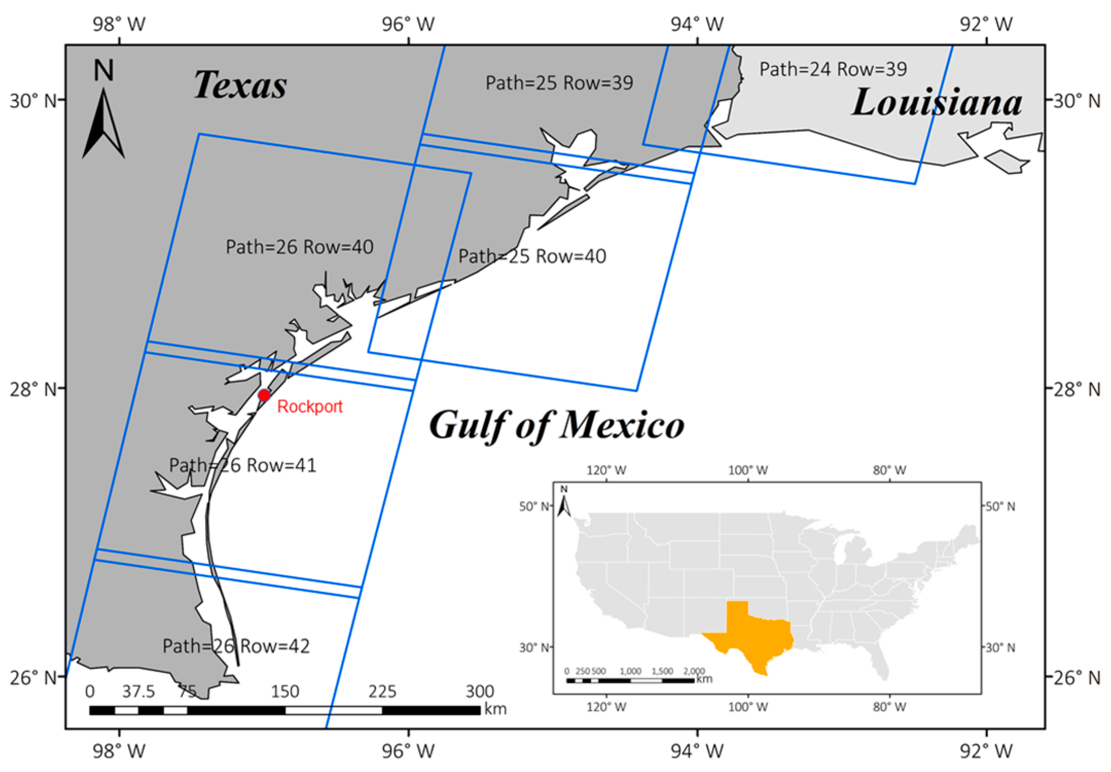
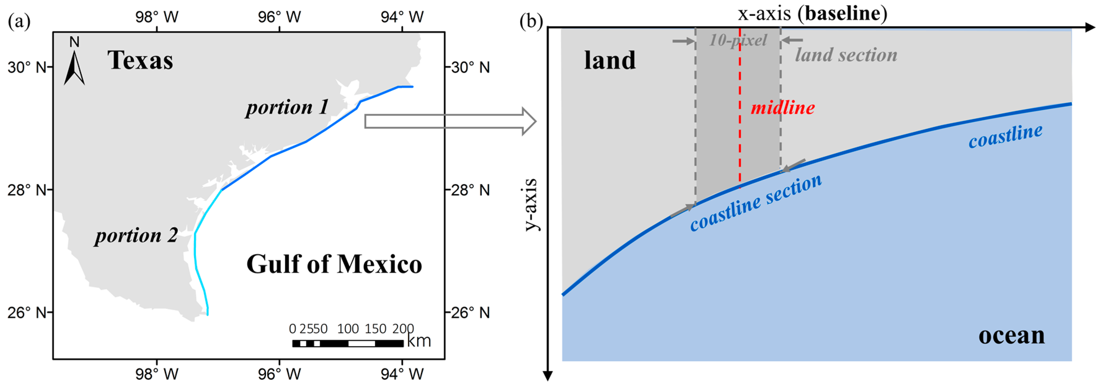
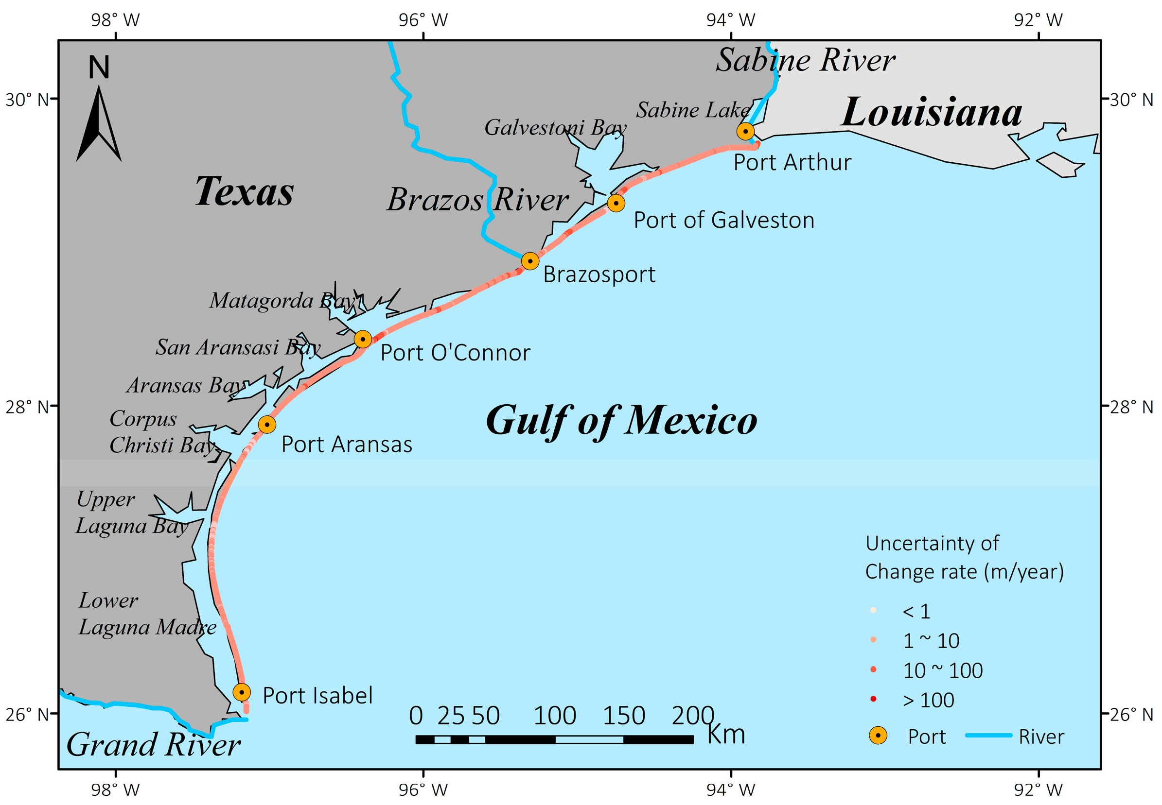
2.1. Study Area
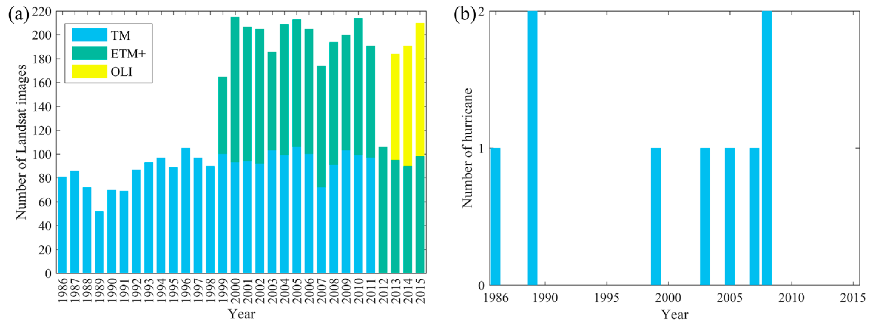
2.2. Remotely Sensed Data
2.3. Validation Data
2.4. Hurricane Data
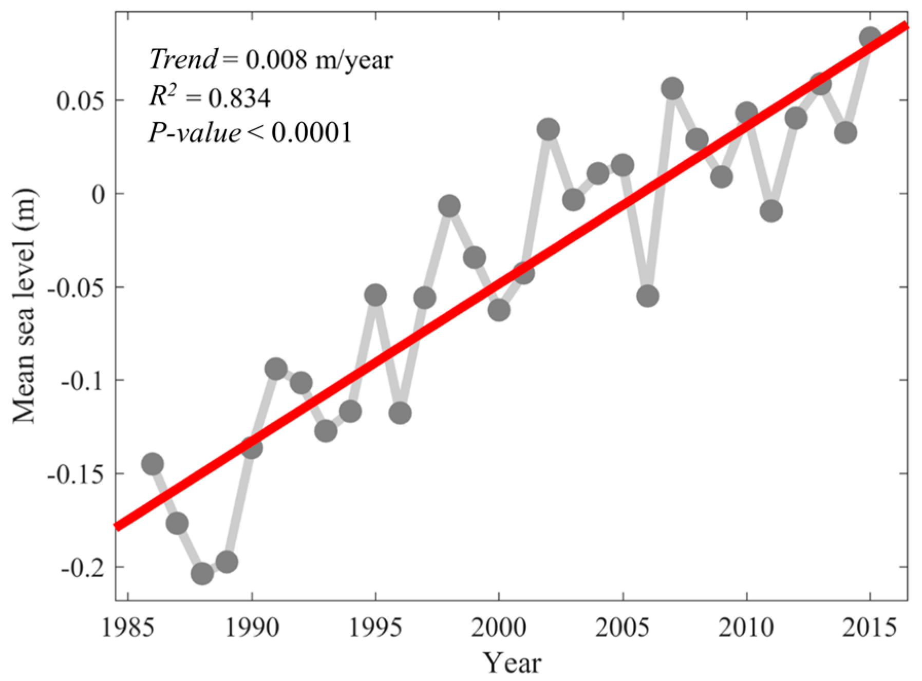
2.5. Sea Level Data
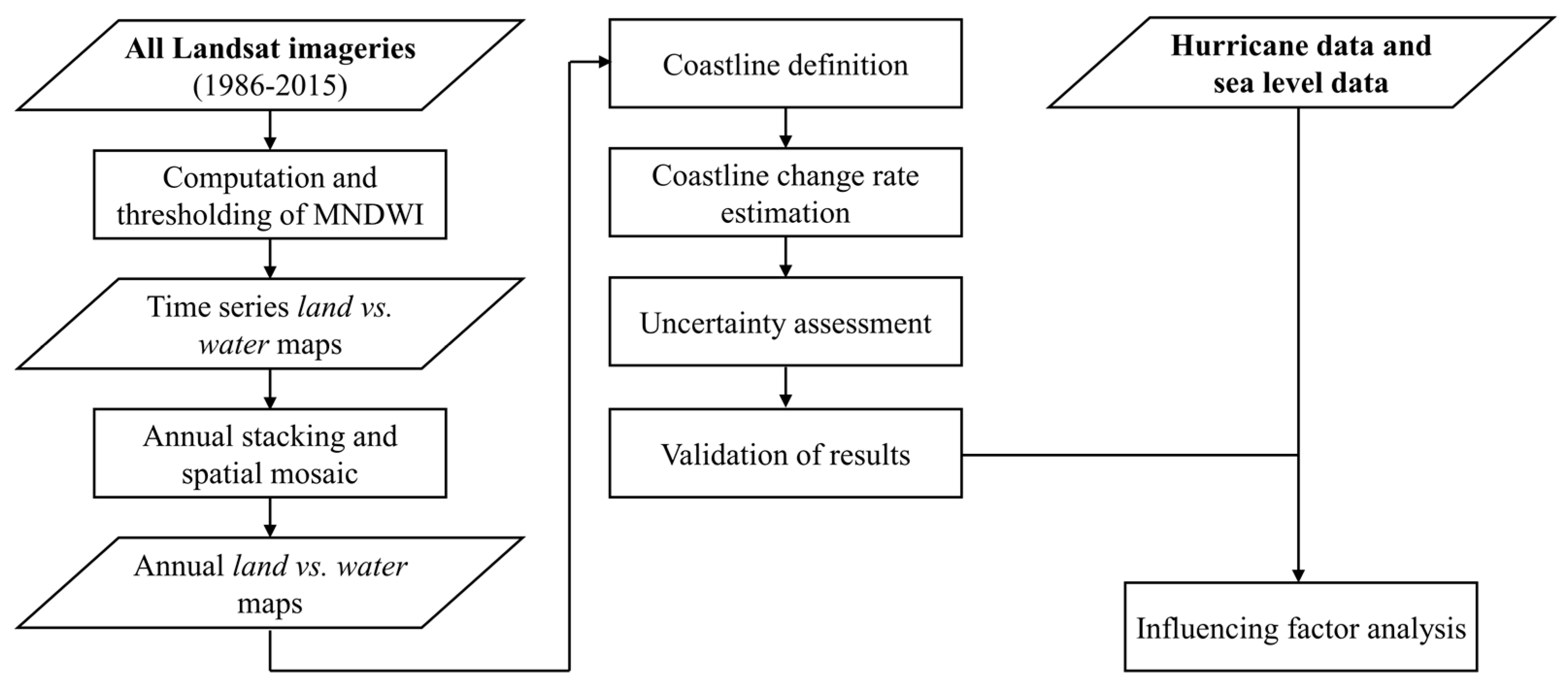
3. Methodology
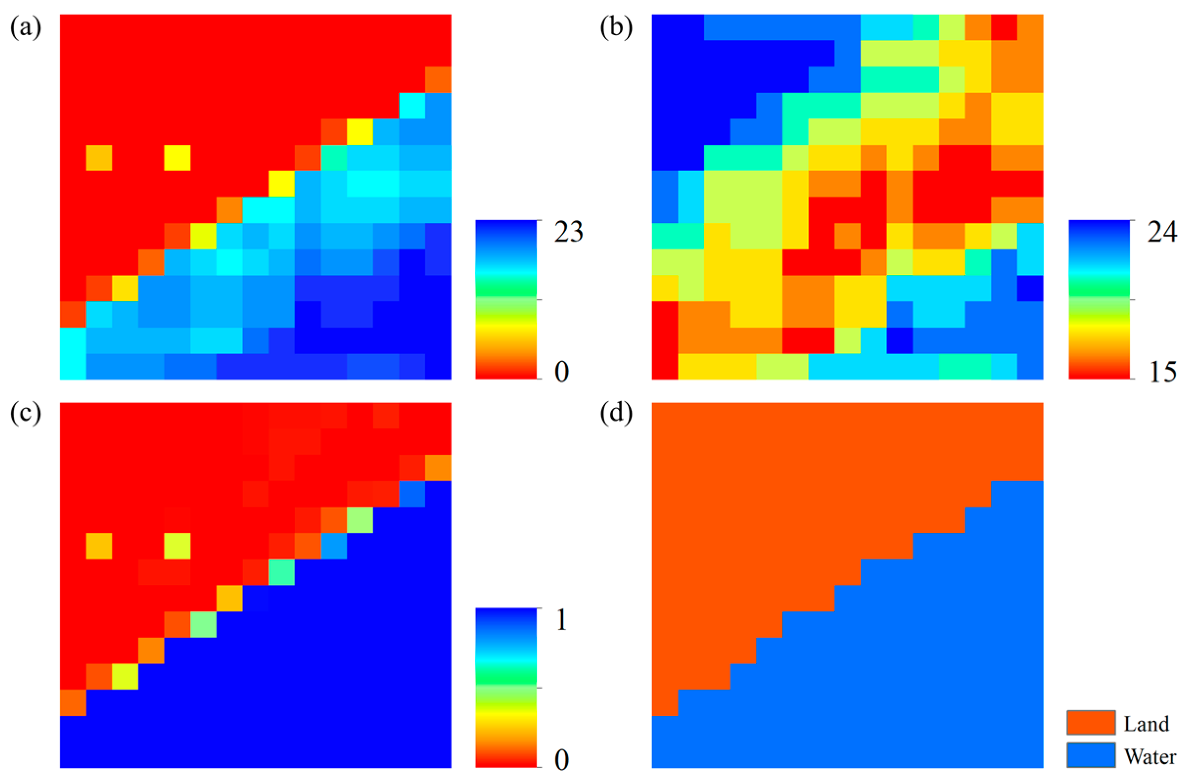
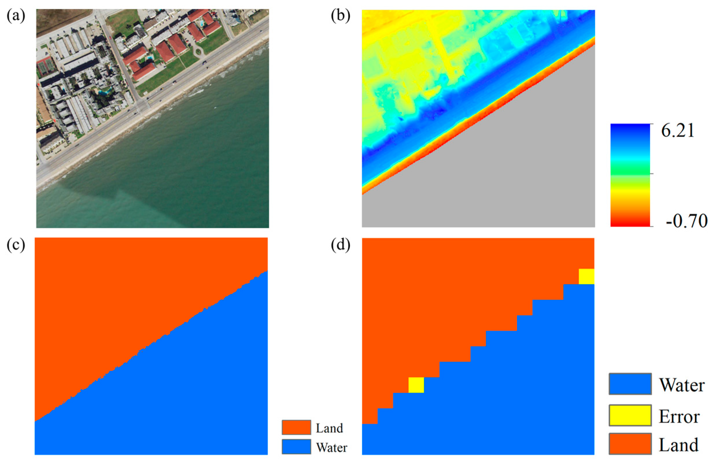
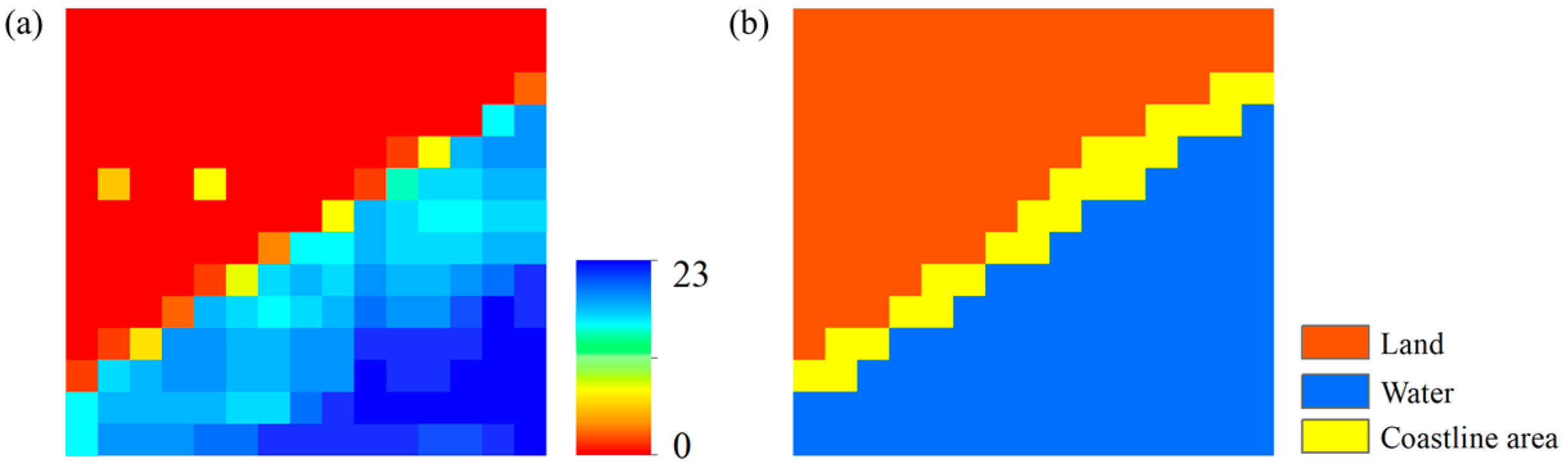
3.1. Annual Land—Water Maps Generation
3.2. Coastline Change Rate Estimation
3.3. Uncertainty Assessment
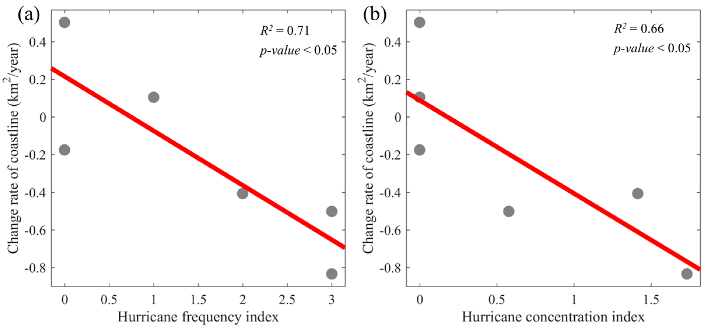
3.4. Impact of Hurricane on Coastline Change
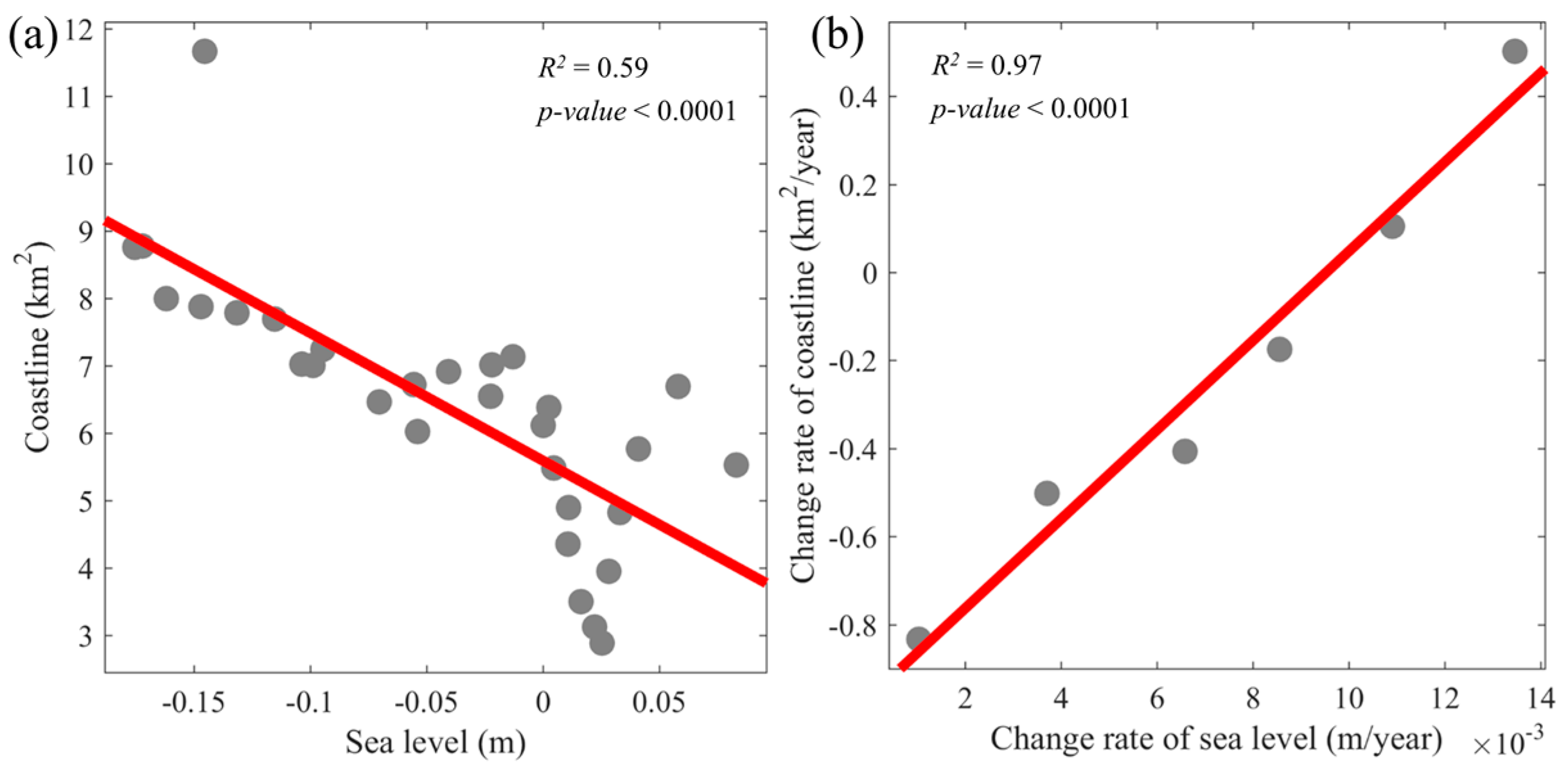
3.5. Impact of Sea Level Variation on Coastline Change
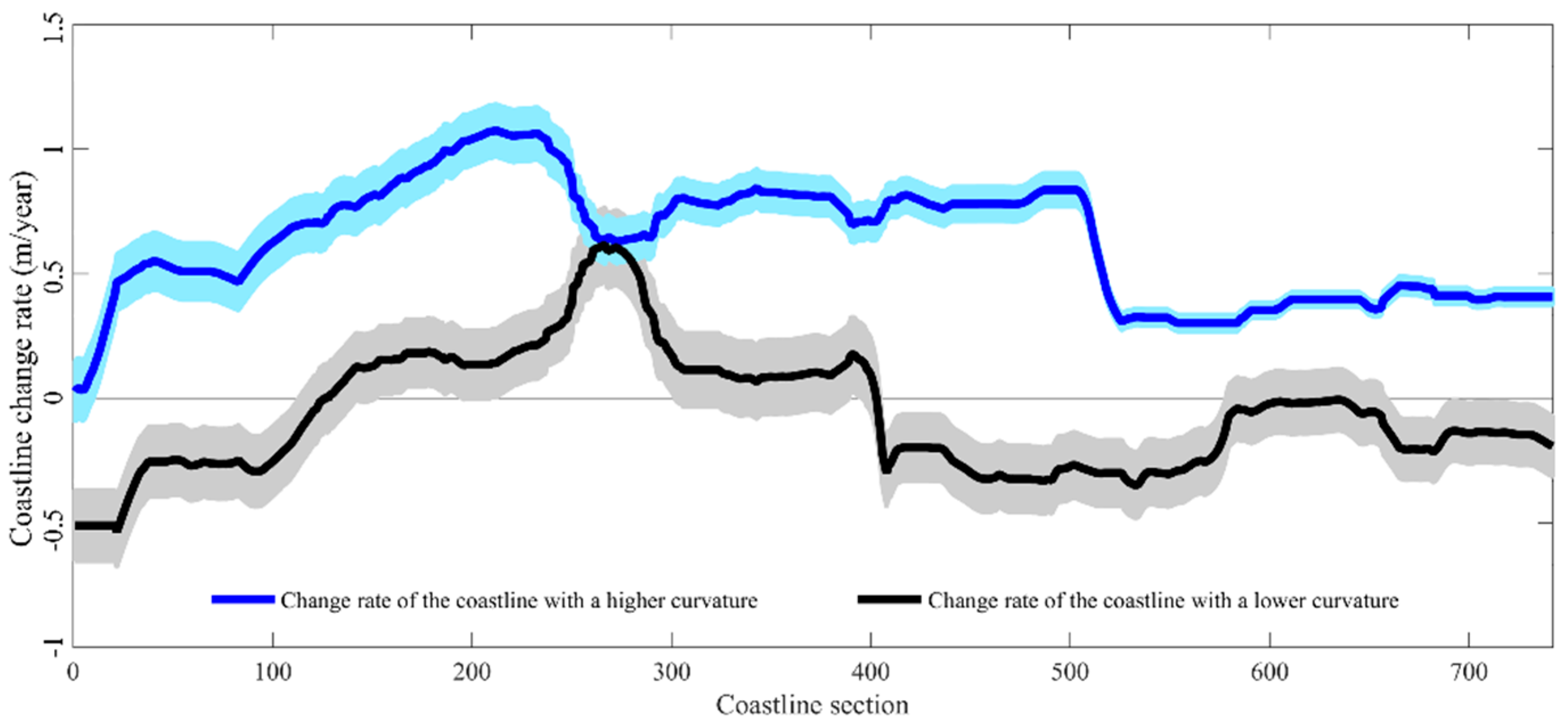
3.6. Coastline Morphology Anlysis
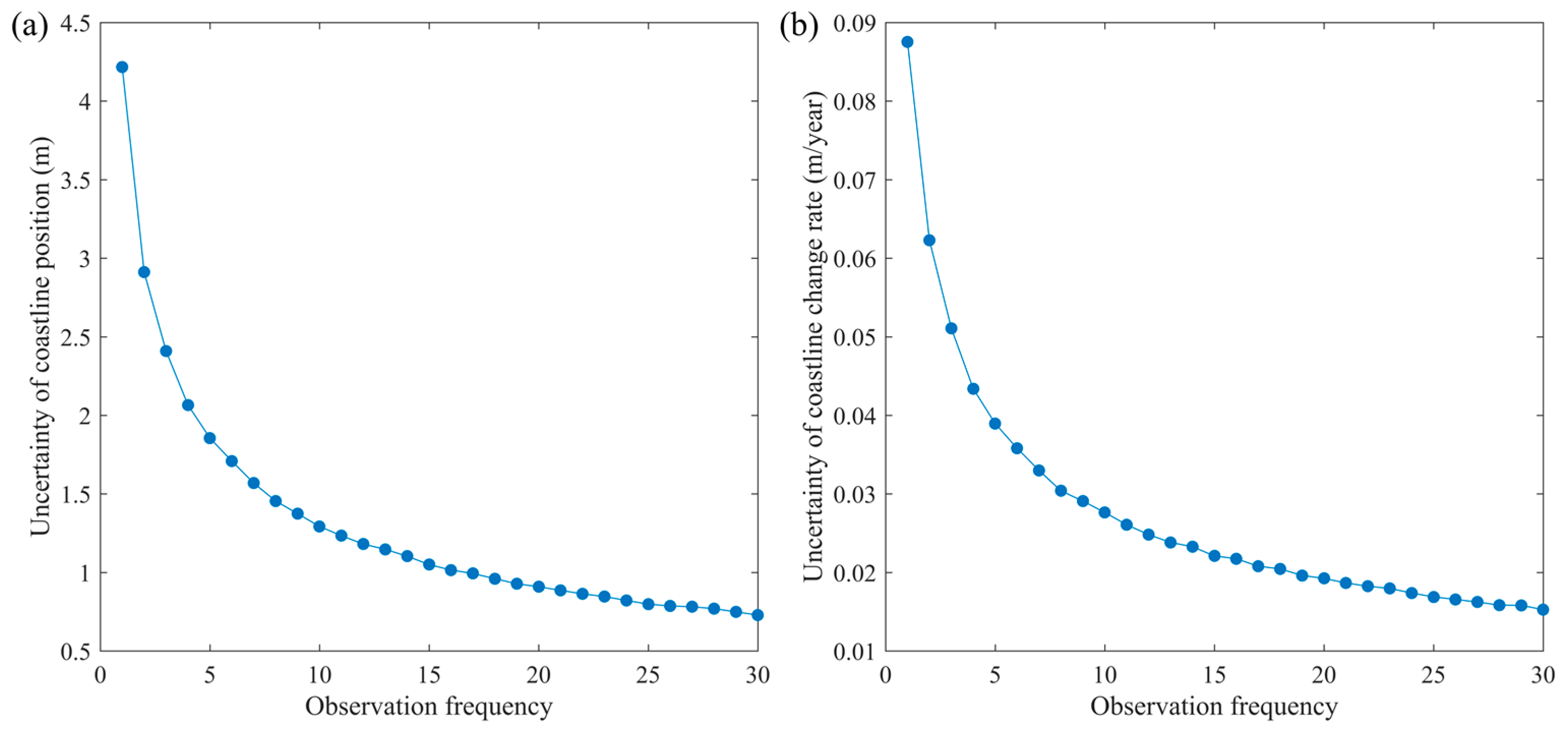
3.7. Effect of Observation Frequency on Estimation of Coastline Change Rate
4. Results
4.1. Spatial Pattern Analysis of Coastline Change
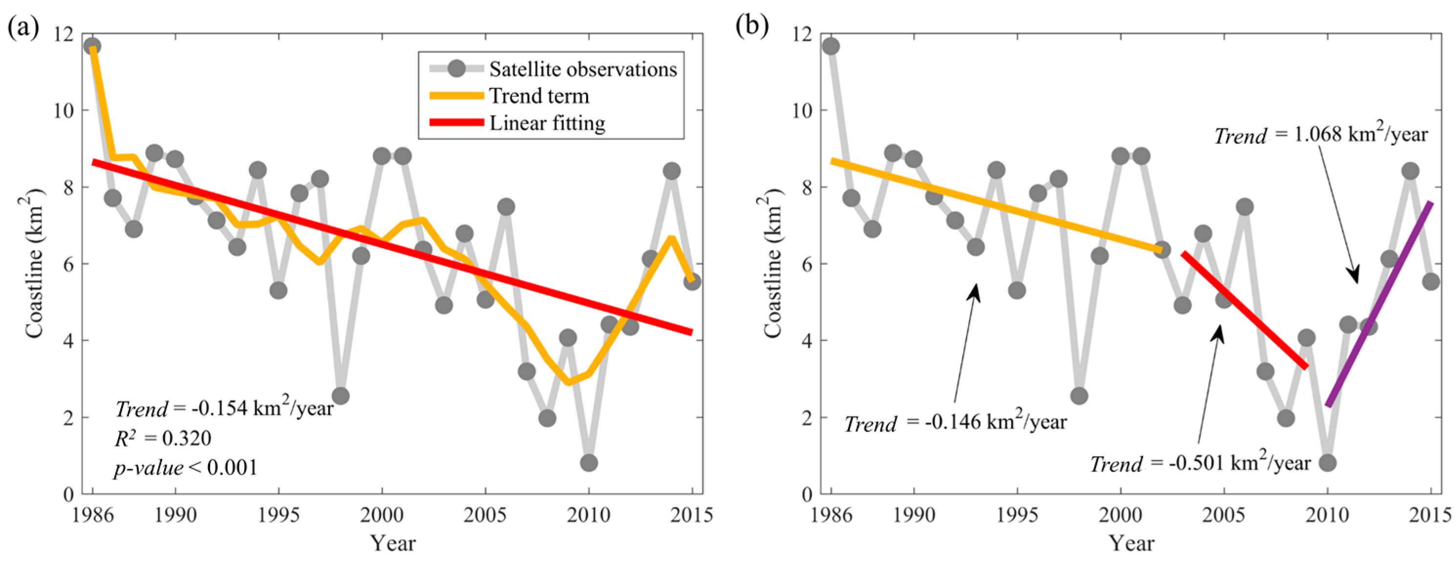
4.2. Temporal Variation Analysis of Coastline Change
4.3. Influencing Factor Analysis
4.4. Validation of Land-Water Map Using LIDAR Data
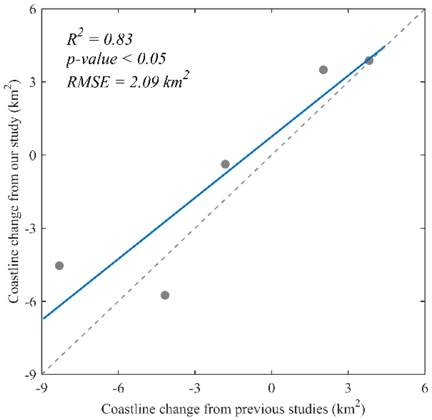
4.5. Validation of Coastline Change in the Texas State
5. Discussions
5.1. Influencing Factors of Coastline Change
5.2. Effect of Observation Frequency on Estimation of Coastline Change Rate
5.3. Further Considerations
6. Conclusions
Acknowledgments
Author Contributions
Conflicts of Interest
References
- Yang, J.; Gong, P.; Fu, R.; Zhang, M.; Chen, J.; Liang, S.; Xu, B.; Shi, J.; Dickinson, R. The role of satellite remote sensing in climate change studies. Nat. Clim. Chang. 2013, 3, 875–883. [Google Scholar] [CrossRef]
- Ranasinghe, R.; Callaghan, D.; Stive, M.J.F. Estimating coastal recession due to sea level rise: Beyond the Bruun rule. Clim. Chang. 2011, 110, 561–574. [Google Scholar] [CrossRef]
- Zhang, K.; Douglas, B.C.; Leatherman, S.P. Global warming and coastal erosion. Clim. Chang. 2004, 64, 41–58. [Google Scholar] [CrossRef]
- Fearnley, S.M.; Miner, M.D.; Kulp, M.; Bohling, C.; Penland, S. Hurricane impact and recovery shoreline change analysis of the Chandeleur Islands, Louisiana, USA: 1855 to 2005. Geo-Mar. Lett. 2009, 29, 455–466. [Google Scholar] [CrossRef]
- Syvitski, J.P.M.; Kettner, A.J.; Overeem, I.; Hutton, E.W.H.; Hannon, M.T.; Brakenridge, G.R.; Day, J.; Vörösmarty, C.; Saito, Y.; Giosan, L.; et al. Sinking deltas due to human activities. Nat. Geosci. 2009, 2, 681–686. [Google Scholar] [CrossRef]
- Jennings, S. Coastal tourism and shoreline management. Ann. Tour. Res. 2004, 31, 899–922. [Google Scholar] [CrossRef]
- Tanaka, N.; Sato, S. Topographic change resulting from construction of a harbor on a beach: Kashima Port. Coast. Eng. 1976, 1977, 1824–1843. [Google Scholar]
- Peterson, C.H.; Bishop, M.J. Assessing the environmental impacts of beach nourishment. Bioscience 2005, 55, 887–896. [Google Scholar] [CrossRef]
- Muttitanon, W.; Tripathi, N.K. Land use/land cover changes in the coastal zone of Ban Don Bay, Thailand using Landsat 5 TM data. Int. J. Remote Sens. 2005, 26, 2311–2323. [Google Scholar] [CrossRef]
- Shalaby, A.; Tateishi, R. Remote sensing and GIS for mapping and monitoring land cover and land-use changes in the northwestern coastal zone of Egypt. Appl. Geogr. 2007, 27, 28–41. [Google Scholar] [CrossRef]
- Defeo, O.; McLachlan, A.; Schoeman, D.S.; Schlacher, T.A.; Dugan, J.; Jones, A.; Lastra, M.; Scapini, F. Threats to beach ecosystems: A review. Estuar. Coast. Shelf Sci. 2009, 81, 1–12. [Google Scholar] [CrossRef]
- Cazenave, A.; Cozannet, G.L. Sea level rise and its coastal impacts. Earth’s Future 2014, 2, 15–34. [Google Scholar] [CrossRef]
- Le Cozannet, G.; Garcin, M.; Yates, M.; Idier, D.; Meyssignac, B. Approaches to evaluate the recent impacts of sea-level rise on shoreline changes. Earth-Sci. Rev. 2014, 138, 47–60. [Google Scholar] [CrossRef]
- Boak, E.H.; Turner, I.L. Shoreline definition and detection: A review. J. Coast. Res. 2005, 214, 688–703. [Google Scholar] [CrossRef]
- Gens, R. Remote sensing of coastlines: Detection, extraction and monitoring. Int. J. Remote Sens. 2010, 31, 1819–1836. [Google Scholar] [CrossRef]
- Thieler, E.R.; Himmelstoss, E.A.; Zichichi, J.L.; Ergul, A. The Digital Shoreline Analysis System (DSAS) Version 4.0-An ArcGIS Extension for Calculating Shoreline Change (No. 2008-1278); US Geological Survey: Reston, VA, USA, 2009.
- Shaw, J.B.; Wolinsky, M.A.; Paola, C.; Voller, V.R. An image-based method for shoreline mapping on complex coasts. Geophys. Res. Lett. 2008, 35, L12405. [Google Scholar] [CrossRef]
- Li, W.; Gong, P. Continuous monitoring of coastline dynamics in western Florida with a 30-year time series of Landsat imagery. Remote Sens. Environ. 2016, 179, 196–209. [Google Scholar] [CrossRef]
- Rahman, A.F.; Dragoni, D.; El-Masri, B. Response of the Sundarbans coastline to sea level rise and decreased sediment flow: A remote sensing assessment. Remote Sens. Environ. 2011, 115, 3121–3128. [Google Scholar] [CrossRef]
- Honeycutt, M.G.; Crowell, M.; Douglas, B.C. Shoreline-position forecasting: Impact of storms, rate-calculation methodologies, and temporal scales. J. Coast. Res. 2001, 17, 721–730. [Google Scholar]
- Karunarathna, H.; Reeve, D.E. A hybrid approach to model shoreline change at multiple timescales. Cont. Shelf Res. 2013, 66, 29–35. [Google Scholar] [CrossRef]
- Ghoneim, E.; Mashaly, J.; Gamble, D.; Halls, J.; AbuBakr, M. Nile delta exhibited a spatial reversal in the rates of shoreline retreat on the Rosetta promontory comparing pre- and post-beach protection. Geomorphology 2015, 228, 1–14. [Google Scholar] [CrossRef]
- Yu, K.; Hu, C.; Muller-Karger, F.E.; Lu, D.; Soto, I. Shoreline changes in west-central Florida between 1987 and 2008 from Landsat observations. Int. J. Remote Sens. 2011, 32, 8299–8313. [Google Scholar] [CrossRef]
- Chen, W.-W.; Chang, H.-K. Estimation of shoreline position and change from satellite images considering tidal variation. Estuar. Coast. Shelf Sci. 2009, 84, 54–60. [Google Scholar] [CrossRef]
- Ford, M. Shoreline changes interpreted from multi-temporal aerial photographs and high resolution satellite images: Wotje atoll, Marshall Islands. Remote Sens. Environ. 2013, 135, 130–140. [Google Scholar] [CrossRef]
- Frihy, O.E.; Dewidar, K.M.; Nasr, S.M.; El Raey, M.M. Change detection of the northeastern Nile Delta of Egypt: Shoreline changes, spit evolution, margin changes of Manzala lagoon and its islands. Int. J. Remote Sens. 1998, 19, 1901–1912. [Google Scholar] [CrossRef]
- Fletcher, C.H.; Romine, B.M.; Genz, A.S.; Barbee, M.M.; Dyer, M.; Anderson, T.R.; Lim, S.C.; Vitousek, S.; Bochicchio, C.; Richmond, B.M. National Assessment of Shoreline Change: Historical Shoreline Change in the Hawaiian Islands; U.S. Department of the Interior: Washington, DC, USA, 2011.
- Stockdonf, H.F.; Holman, R.A. Estimation of shoreline position and change using airborne topographic lidar data. J. Coast. Res. 2002, 18, 502–513. [Google Scholar]
- Pianca, C.; Holman, R.; Siegle, E. Shoreline variability from days to decades: Results of long-term video imaging. J. Geophys. Res. Oceans 2015, 120, 2159–2178. [Google Scholar] [CrossRef]
- Harley, M.D.; Turner, I.L.; Short, A.D.; Ranasinghe, R. Assessment and integration of conventional, RTK-GPS and image-derived beach survey methods for daily to decadal coastal monitoring. Coast. Eng. 2011, 58, 194–205. [Google Scholar] [CrossRef]
- Gong, P. Remote sensing of environmental change over China: A review. Chin. Sci. Bull. 2012, 57, 2793–2801. [Google Scholar] [CrossRef]
- Hui, F.; Xu, B.; Huang, H.; Yu, Q.; Gong, P. Modelling spatial-temporal change of Poyang Lake using multitemporal Landsat imagery. Int. J. Remote Sens. 2008, 29, 5767–5784. [Google Scholar] [CrossRef]
- Kovalskyy, V.; Roy, D.P. The global availability of Landsat 5 TM and Landsat 7 ETM+ land surface observations and implications for global 30 m Landsat data product generation. Remote Sens. Environ. 2013, 130, 280–293. [Google Scholar] [CrossRef]
- Almonacid-Caballer, J.; Sánchez-García, E.; Pardo-Pascual, J.E.; Balaguer-Beser, A.A.; Palomar-Vázquez, J. Evaluation of annual mean shoreline position deduced from Landsat imagery as a mid-term coastal evolution indicator. Mar. Geol. 2016, 372, 79–88. [Google Scholar] [CrossRef]
- Leatherman, S.P. Coastal geomorphic responses to sea-level Rise, Galveston Bay, Texas. In Greenhouse Effect and Sea-Level Rise: A Challenge for this Generation; Barth, M.C., Titus, J.G., Eds.; Van Nostrand Reinhold: New York, NY, USA, 1984; pp. 151–178. [Google Scholar]
- Paine, J.G.; Caudle, T.L.; Andrews, J.R. Shoreline and sand storage dynamics from annual airborne Lidar surveys, Texas Gulf coast. J. Coast. Res. 2017, 33, 487–506. [Google Scholar] [CrossRef]
- Sea Level Trends. Available online: https://tidesandcurrents.noaa.gov/ (accessed on 1 July 2015).
- Roth, D. Texas Hurricane History; Long Island Business News: New York, NY, USA, 2006. [Google Scholar]
- Effect of Hurricane Ike in Texas. Available online: https://en.wikipedia.org/wiki/Effects_of_Hurricane_Ike_in_Texas#cite_note-YNaft-2 (accessed on 1 July 2015).
- Zane, D.F.; Bayleyegn, T.M.; Hellsten, J.; Beal, R.; Beasley, C.; Haywood, T.; Wiltz-beckham, D.; Wolkin, A.F. Tracking deaths related to hurricane Ike, Texas, 2008. Disaster Med. Public Health Prep. 2011, 5, 23–28. [Google Scholar] [CrossRef] [PubMed]
- Center, N.H. Tropical Cyclone Report Hurricane Ike (al092008) 1–14 September 2008; National Hurricane Center: Gainesville, FL, USA, 2008. [Google Scholar]
- Song, C.; Woodcock, C.E.; Seto, K.C.; Lenney, M.P.; Macomber, S.A. Classification and change detection using Landsat TM data: when and how to correct atmospheric effects? Remote Sens. Environ. 2001, 75, 230–244. [Google Scholar] [CrossRef]
- Lin, C.; Wu, C.C.; Tsogt, K.; Ouyang, Y.C.; Chang, C.I. Effects of atmospheric correction and pansharpening on LULC classification accuracy using WorldView-2 imagery. Inf. Process. Agric. 2015, 2, 25–36. [Google Scholar] [CrossRef]
- Unisys Weather Information System. Available online: http://weather.unisys.com/hurricane/ (accessed on 1 July 2015).
- Fitzgerald, D.M.; Fenster, M.S.; Argow, B.A.; Buynevich, I.V. Coastal impacts due to sea-level rise. Annu. Rev. Earth Planet. Sci. 2007, 36, 601–647. [Google Scholar] [CrossRef]
- Real-time Water Level Information in the USA. Available online: https://tidesandcurrents.noaa.gov/stations.html?type=Water+Levels (accessed on 1 July 2015).
- Zhu, Z.; Woodcock, C.E. Object-based cloud and cloud shadow detection in Landsat imagery. Remote Sens. Environ. 2012, 118, 83–94. [Google Scholar] [CrossRef]
- Cui, B.L.; Li, X.Y. Coastline change of the Yellow River estuary and its response to the sediment and runoff (1976–2005). Geomorphology 2011, 127, 32–40. [Google Scholar] [CrossRef]
- Li, Y.; Gong, X.; Guo, Z.; Xu, K.; Hu, D.; Zhou, H. An index and approach for water extraction using Landsat-OLI data. Int. J. Remote Sens. 2016, 37, 3611–3635. [Google Scholar] [CrossRef]
- Kelly, J.T.; Gontz, A.M. Using GPS-surveyed intertidal zones to determine the validity of shorelines automatically mapped by Landsat water indices. Int. J. Appl. Earth Obs. Geoinf. 2018, 65, 92–104. [Google Scholar] [CrossRef]
- Xu, H. Modification of Normalised Difference Water Index (NDWI) to enhance open water features in remotely sensed imagery. Int. J. Remote Sens. 2006, 27, 3025–3033. [Google Scholar] [CrossRef]
- Sagin, J.; Sizo, A.; Wheater, H.; Jardine, T.D.; Lindenschmidt, K.E. A water coverage extraction approach to track inundation in the Saskatchewan River Delta, Canada. Int. J. Remote Sens. 2015, 36, 764–781. [Google Scholar] [CrossRef]
- Acharya, T.; Yang, I.T.; Subedi, A.; Lee, D.H. Change detection of Lakes in Pokhara, Nepal using Landsat Data. In Proceedings of the 3rd International Electronic Conference on Sensors and Applications, online, 15–30 November 2016. [Google Scholar]
- Fisher, A.; Flood, N.; Danaher, T. Comparing Landsat water index methods for automated water classification in Eastern Australia. Remote Sens. Environ. 2016, 175, 167–182. [Google Scholar] [CrossRef]
- Sagar, S.; Roberts, D.; Bala, B.; Lymburner, L. Extracting the intertidal extent and topography of the Australian coastline from a 28 year time series of Landsat observations. Remote Sens. Environ. 2017, 195, 153–169. [Google Scholar] [CrossRef]
- Romine, B.M.; Fletcher, C.H.; Frazer, L.N.; Genz, A.S.; Barbee, M.M.; Lim, S.C. Historical shoreline change, southeast Oahu, Hawaii; applying polynomial models to calculate shoreline change rates. J. Coast. Res. 2009, 25, 1236–1253. [Google Scholar] [CrossRef]
- Houser, C.; Hapke, C.; Hamilton, S. Controls on coastal dune morphology, shoreline erosion and barrier island response to extreme storms. Geomorphology 2008, 100, 223–240. [Google Scholar] [CrossRef]
- Ozturk, D.; Beyazit, I.; Kilic, F. Spatiotemporal analysis of shoreline changes of the Kizilirmak Delta. J. Coast. Res. 2014, 31, 1389–1402. [Google Scholar] [CrossRef]
- Filho, P.W.M.S.; Martins, E.D.S.F.; Costa, F.R.D. Using mangroves as a geological indicator of coastal changes in the Bragança macrotidal flat, Brazilian Amazon: A remote sensing data approach. Ocean Coast. Manag. 2006, 49, 462–475. [Google Scholar] [CrossRef]
- Chu, Z.X.; Sun, X.G.; Zhai, S.K.; Xu, K.H. Changing pattern of accretion/erosion of the modern Yellow River (Huanghe) subaerial delta, China: Based on remote sensing images. Mar. Geol. 2006, 227, 13–30. [Google Scholar] [CrossRef]
- El-Raey, M.; Sharaf El-Din, S.H.; Khafagy, A.A.; Abo Zed, A.I. Remote sensing of beach erosion / accretion patterns along Damietta-port said shoreline, Egypt. Int. J. Remote Sens. 1999, 20, 1087–1106. [Google Scholar] [CrossRef]
- Liao, E.; Lu, W.; Yan, X.H.; Jiang, Y.; Kidwell, A. The coastal ocean response to the global warming acceleration and hiatus. Sci. Rep. 2015, 5, 16630. [Google Scholar] [CrossRef] [PubMed]
- Puig, M.; del Rio, L.; Plomaritis, T.A.; Benavente, J. Influence of storms on coastal retreat in SW Spain. J. Coast. Res. 2014, 70, 193–198. [Google Scholar] [CrossRef]
- Anderson, T.R.; Frazer, L.N.; Fletcher, C.H. Transient and persistent shoreline change from a storm. Geophys. Res. Lett. 2010, 37, 162–169. [Google Scholar] [CrossRef]
- Nebel, S.H.; Trembanis, A.C.; Barber, D.C. Tropical cyclone frequency and barrier island erosion rates, Cedar Island, Virginia. J. Coast. Res. 2013, 286, 133–144. [Google Scholar] [CrossRef]
- Bruun, P. The Bruun rule of erosion by sea-level rise: A discussion on large-scale two-and three-dimensional usages. J. Coast. Res. 1988, 4, 627–648. [Google Scholar]
- Splinter, K.D.; Turner, I.L.; Davidson, M.A. How much data is enough? The importance of morphological sampling interval and duration for calibration of empirical shoreline models. Coast. Eng. 2013, 77, 14–27. [Google Scholar] [CrossRef]
- Reif, M.K.; Macon, C.L.; Wozencraft, J.M. Post-Katrina land-cover, elevation, and volume change assessment along the south shore of lake Pontchartrain, Louisiana, U.S.A. J. Coast. Res. 2011, 62, 30–39. [Google Scholar] [CrossRef]
- Paine, J.G.; Caudle, T.L.; Andrews, J.L. Shoreline Movement along the Texas Gulf Coast, 1930’s to 2012; Final Report to the Texas General Land Office, Bureau of Economic Geology; the University of Texas: Austin, TX, USA, 2014. [Google Scholar]
- Paine, J.G.; Mathew, S.; Caudle, T. Historical shoreline change through 2007, Texas Gulf Coast: Rates, contributing causes, and Holocene context. Gcags J. 2012, 1, 13–26. [Google Scholar]
- Morton, R.A.; Miller, T.L.; Moore, L.J. National Assessment of Shoreline Change: Part 1 Historical Shoreline Changes and Associated Coastal Land Loss along the U.S. Gulf of Mexico; USGS—U.S. Geological Survey, Center for Coastal & Regional Marine Studies: Reston, VA, USA, 2004.
- Morton, R.A. Stages and durations of post-storm beach recovery, Southeastern Texas Coast, U.S.A. J. Coast. Res. 1994, 10, 884–908. [Google Scholar]
- Frazer, L.N.; Anderson, T.R.; Fletcher, C.H. Modeling storms improves estimates of long-term shoreline change. Geophys. Res. Lett. 2009, 37, 1437–1454. [Google Scholar] [CrossRef]
- Coco, G.; Senechal, N.; Rejas, A.; Bryan, K.R.; Capo, S.; Parisot, J.P.; Brown, J.A.; MacMahan, J.H.M. Beach response to a sequence of extreme storms. Geomorphology 2014, 204, 493–501. [Google Scholar] [CrossRef]
- Óscar, F. Storm groups versus extreme single storms: Predicted erosion and management consequences. J. Coast. Res. 2005, 21, 221–227. [Google Scholar]
- Mulcahy, N.; Kennedy, D.M.; Blanchon, P. Hurricane-induced shoreline change and post-storm recovery: Northeastern Yucatan Peninsula, Mexico. J. Coast. Res. 2016, 2, 1192–1196. [Google Scholar] [CrossRef]
- Leatherman, S.P.; Zhang, K.; Douglas, B.C. Sea level rise shown to drive coastal erosion. Eos Trans. Am. Geophys. Union 2000, 81, 55–57. [Google Scholar] [CrossRef]
- Bullard, F.M. Source of beach and river sands on gulf coast of Texas. Geol. Soc. Am. Bull. 1942, 53, 1021–1043. [Google Scholar] [CrossRef]
- Ells, K.D. Convexity, Concavity, and Human Agency in Large-Scale Coastline Evolution. Ph.D. Thesis, Duke University, Durham, NC, USA, 2014. [Google Scholar]
- Phillips, J.D. Erosion and Planform Irregularity of an Estuarine Shoreline. Zeitschrift fiir Geomorphologie; Gerbruder Borntr: Berlin, Germany, 1989; pp. 59–71. [Google Scholar]
- Letetrel, C.; Karpytchev, M.; Bouin, M.N.; Marcos, M.; Santamaríagómez, A.; Wöppelmann, G. Estimation of vertical land movement rates along the coasts of the Gulf of Mexico over the past decades. Cont. Shelf Res. 2015, 111, 42–51. [Google Scholar] [CrossRef]


| Path/Row | Level | Scene Amount per Sensor | Total Amount per Scene | ||
|---|---|---|---|---|---|
| TM | ETM+ | OLI | |||
| 024/039 | L1T | 372 | 284 | 48 | 704 |
| 025/039 | L1T | 396 | 279 | 53 | 730 |
| 025/040 | L1T | 387 | 286 | 47 | 722 |
| 026/040 | L1T | 379 | 282 | 50 | 719 |
| 026/041 | L1T | 369 | 288 | 52 | 719 |
| 026/042 | L1T | 401 | 299 | 52 | 763 |
© 2018 by the author. Licensee MDPI, Basel, Switzerland. This article is an open access article distributed under the terms and conditions of the Creative Commons Attribution (CC BY) license (http://creativecommons.org/licenses/by/4.0/).
Share and Cite
Xu, N. Detecting Coastline Change with All Available Landsat Data over 1986–2015: A Case Study for the State of Texas, USA. Atmosphere 2018, 9, 107. https://doi.org/10.3390/atmos9030107
Xu N. Detecting Coastline Change with All Available Landsat Data over 1986–2015: A Case Study for the State of Texas, USA. Atmosphere. 2018; 9(3):107. https://doi.org/10.3390/atmos9030107
Chicago/Turabian StyleXu, Nan. 2018. "Detecting Coastline Change with All Available Landsat Data over 1986–2015: A Case Study for the State of Texas, USA" Atmosphere 9, no. 3: 107. https://doi.org/10.3390/atmos9030107
APA StyleXu, N. (2018). Detecting Coastline Change with All Available Landsat Data over 1986–2015: A Case Study for the State of Texas, USA. Atmosphere, 9(3), 107. https://doi.org/10.3390/atmos9030107