Activity Characteristics of the East Asian Trough in CMIP5 Models

Abstract

In this paper, the performances of 12 CMIP5 (Coupled Model Intercomparison Project phase 5) models for simulating the climatology and interannual variability of the East Asian trough (EAT) are assessed using the National Centers for Environmental Prediction (NCEP) reanalysis data and the outputs of the CMIP5 models. The multimodel ensemble (MME) successfully reproduces the spatial pattern and spatial variations in the climatology and interannual variability of the EAT but the intensity and interannual variability of EAT are weaker than in the observations. The biases in intensity (interannual variability) are larger over the southern (northern) part of the EAT than over the northern (southern) part. The intermodel spreads are small for the EAT intensity but are large for its location in terms of both latitude and longitude. The simulated EAT in the MME is about 3° E and 1.5° S of that observed. All 12 CMIP5 models reproduce the first empirical orthogonal function (EOF) mode of EAT activity; however, its intensity and location are only successfully captured in half of the models and its linear weakening trend is simulated in ten models. The second EOF mode of EAT activity and its linear strengthening trend are successfully reproduced in eight models.

1. Introduction

The East Asian trough (EAT) is a quasi-stationary planetary trough at mid-level troposphere over the northern part of the East Asian monsoon region and is an important component of the East Asian winter monsoon (EAWM, [1,2]). EAT has prominent seasonal, interannual, and interdecadal variations. Its seasonal variation is closely related to the establishment and retreat of the EAWM circulation [3,4], while its interannual variation may reflect the intensity of the EAWM. A deepened EAT may lead to a stronger intrusion of cold air into low latitudes from high latitudes, which results in the cold waves, freezing rain, and snow disasters, creating hazards to human livelihoods in East Asia [5,6,7,8,9]. Many studies have reported the decadal weakening of EAT intensity and its eastward shift during the late 1970s [10,11], which are related to the decadal weakening of the EAWM. The two leading modes of EAT activity were identified by Wang et al. [1] using the empirical orthogonal function (EOF) analysis. The first EOF mode shows the variation of the EAT intensity and the second EOF mode represents the variation of the EAT axis.

The activity of EAT is also influenced by the Arctic Oscillation (AO) and El Niño-Southern Oscillation (ENSO). During the negative phase of AO, the intensity of EAT is enhanced, indicating an enhanced EAWM and more powerful cold northerlies [12]. Before the El Niño occurs, the activity of EAT is enhanced, which could enhance the convection over the tropical Western Pacific and promote the development of El Niño [13,14,15]. However, during the El Niño winter, the activity of EAT is weakened due to the anomalous southerlies over the Northwestern Pacific induced by El Niño [14]. Therefore, the EAT plays an important role in connecting the weather and climate variations between the tropics and high latitudes [9,16]. Further study on the activity of EAT is required and this may benefit the weather and climate forecasting.

Numerical climate models are important tools for studying the EAWM and EAT. Ji et al. [17] simulated the interannual variability of the EAWM and its relationship with the sea surface temperature (SST) anomalies over tropical oceans using a single atmospheric general circulation model (AGCM). Li et al. [18] evaluated the performances of a GCM model in simulating the interdecadal variations of EAT. When the observed SST are used in the GCM, the 10–30-year and more than 30-year interdecadal oscillations of EAT can be simulated. The decadal weakening of EAT is also captured by most of the coupled climate models in IPCC AR4 [19]. Under a global warming scenario, the EAT becomes shallower and shifts northeastward in the coupled climate models [20,21,22,23]. The performances of the models in the Coupled Model Intercomparison Project phase 5 (CMIP5) in simulating EAWM are better than those in CMIP3 [23]. The multimodel ensemble (MME) of CMIP5 models is able to reproduce the overall characteristics of EAWM very well [24,25], although the climatological strength of the EAT is overestimated by most of the models [23,24]. However, the performances of CMIP5 models in the variation of EAT are unclear. This gives rise to the question of whether the two leading activity modes of EAT are captured by the CMIP5 models. Assessing the performances of CMIP5 models in simulating the activity of EAT is important for studies on East Asian climate. On the one hand, it is the bases of accurate simulation and prediction of the EAT. On the other hand, it helps us to understand the deficiencies of the climate models in detail and consequently to improve the climate models. Therefore, this paper is mainly studying the above issues using NCEP reanalysis data and the outputs of 12 CMIP5 models. The remainder of this paper is organized as follows. Data and methods are described in Section 2. The climatology and interannual variability of EAT and its two leading EOF modes in the CMIP5 models are investigated in Section 3. Finally, conclusions are provided in Section 4.

2. Data and Methods

Monthly mean atmospheric data of the geopotential height at 500 hPa are from the National Centers for Environmental Prediction/National Center for Atmospheric Research (NCEP/NCAR, [26]) with a horizontal resolution of 2.5° × 2.5°. The CMIP5 models used in this paper and related information are listed in

Table 1. List of the Coupled Model Intercomparison Project phase 5 (CMIP5) models used in this study. The atmospheric resolution refers to the number of grid points in each direction (Lat. × Lon.).

Model	Institute, Country	Atmospheric Resolution
Australian Community Climate and Earth-System Simulator, version 1–3 (ACCESS1-3)	BOM, Australia	192 × 145
Second Generation Canadian Earth System Model (CanESM2)	Canadian Centre for Climate Modelling and Analysis (CCCma), Canada	128 × 64
Centro Euro-Mediterraneo per I Cambiamenti Climatici Climate Model (CMCC-CM)	Centro Euro-Mediterraneo per I Cambiamenti Climatici (CMCC), Italy	192 × 96
Centre National de Recherches Météorologiques Coupled Global Climate Model, version 5 (CNRM-CM5)	Centre National de Recherches Météorologiques (CNRM)-Centre Européen de Recherche et de Formation Avancée en Calcul Scientifique (CERFACS), France	256 × 128
Flexible Global Ocean-Atmosphere-Land System Model (FGOALS) gridpoint, version 2 (FGOALS-g2)	State Key Laboratory of Numerical Modeling for Atmospheric Sciences and Geophysical Fluid Dynamics (LASG), Institute of Atmospheric Physics, Chinese Academy of Sciences and CESS, Tsinghua University, China	120 × 60
FGOALS, second spectral version (FGOALS-s2)	LASG, Institute of Atmospheric Physics, Chinese Academy of Sciences, China	128 × 108
Geophysical Fluid Dynamics Laboratory Climate Model, version 3 (GFDL-CM3)	National Oceanic and Atmospheric Administration (NOAA)/Geophysical Fluid Dynamics Laboratory (GFDL), United States	144 × 90
L’Institut Pierre-Simon Laplace Coupled Model, version 5B, coupled with NEMO, low resolution (IPSL-CM5B-LR)	L’Institut Pierre-Simon Laplace (IPSL), France	96 × 96
Model for Interdisciplinary Research on Climate, version 5 (MIROC5)	Atmosphere and Ocean Research Institute (AORI)-National Institute for Environmental Studies (NIES)-Japan Agency for Marine-Earth Science and Technology (JAMSTEC), Japan	256 × 128
Max Planck Institute Earth System Model, low resolution (MPI-ESM-LR)	Max Planck Institute for Meteorology (MPI-M), Germany	192 × 96
Meteorological Research Institute Coupled Atmosphere–Ocean General Circulation Model, version 3 (MRI CGCM3)	Meteorological Research Institute (MRI), Japan	320 × 160
Norwegian Earth System Model, version 1 (intermediate resolution) (NorESM1-M)	Norwegian Climate Centre, Norway	144 × 96

. The historical experiment was used in this study. Since the horizontal resolution differs from model to model, to compare with the NCEP data, all of the model data were interpolated to match the NCEP reanalysis data resolution. The evaluation is based on the period from January 1950 to December 2005. The results based on NCEP reanalysis data are considered as the observations.

The anomaly of a given variable was generated by removing its climatological mean. Correlation and empirical orthogonal function (EOF) analyses were used and the boreal winter is from December to the following February. The multimodel ensemble (MME) is the average of the 12 CMIP5 models with equal weight.

3. Results

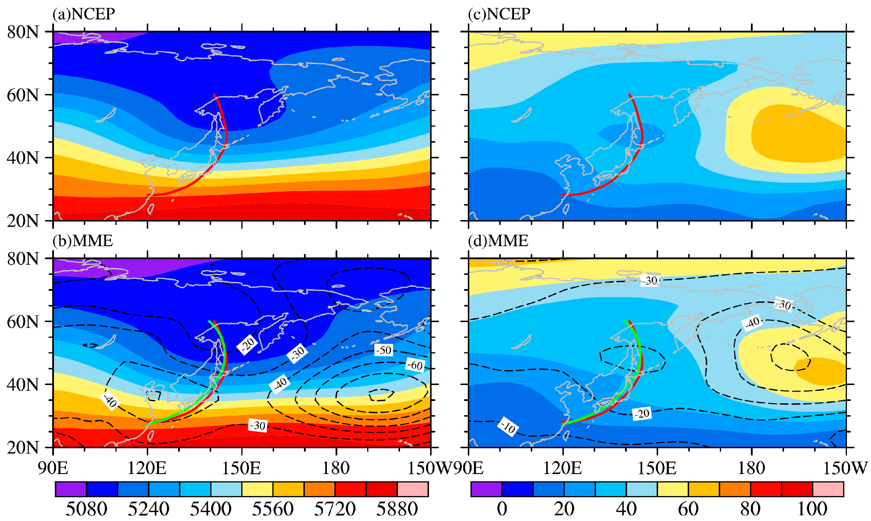
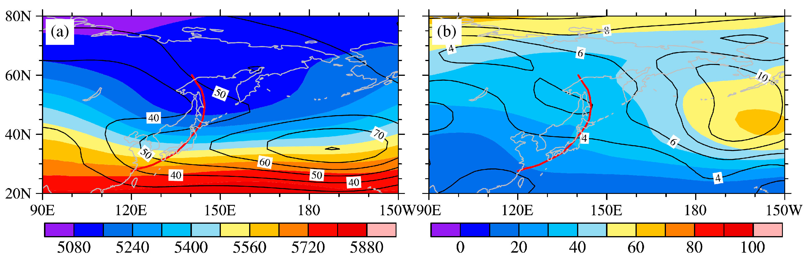
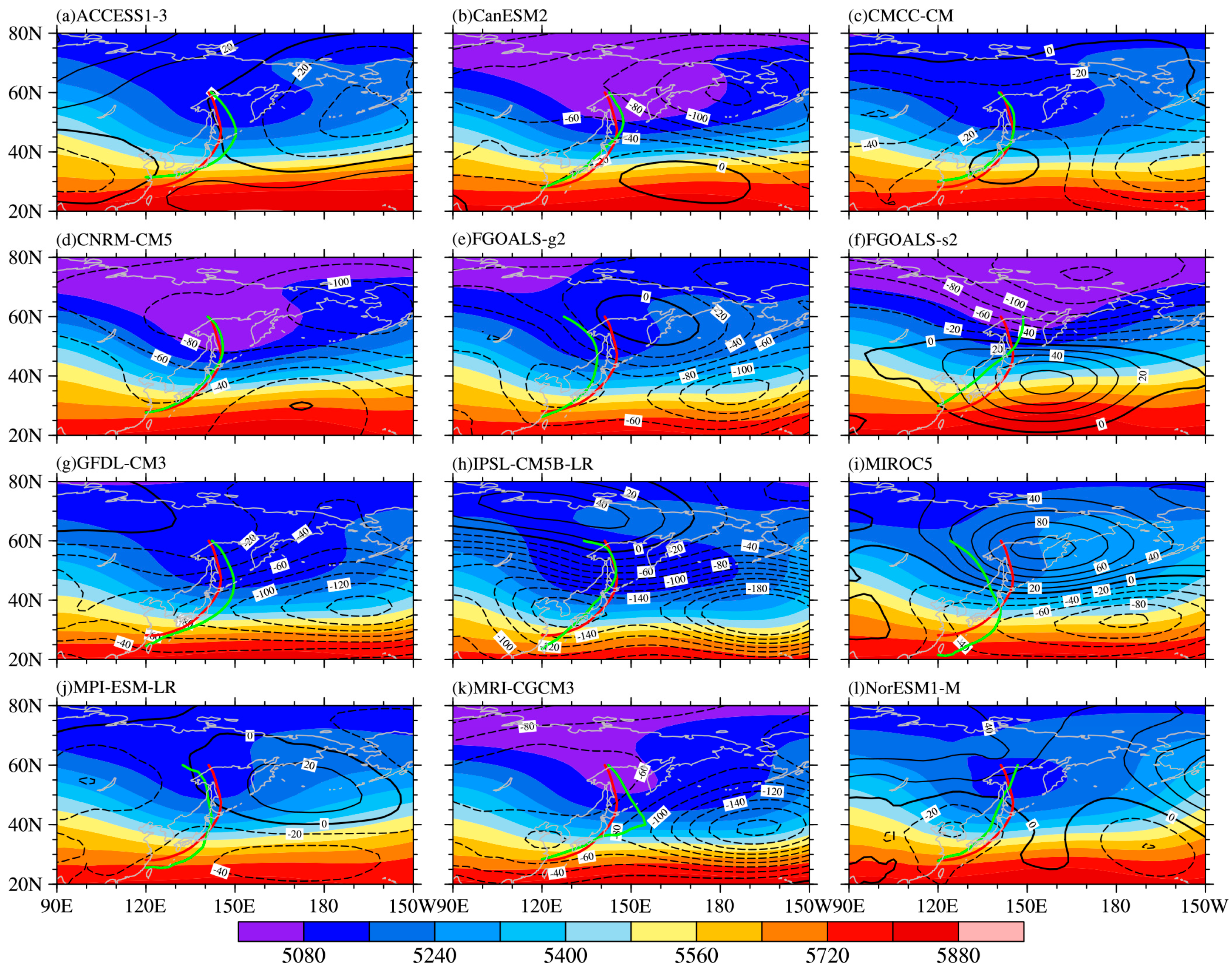
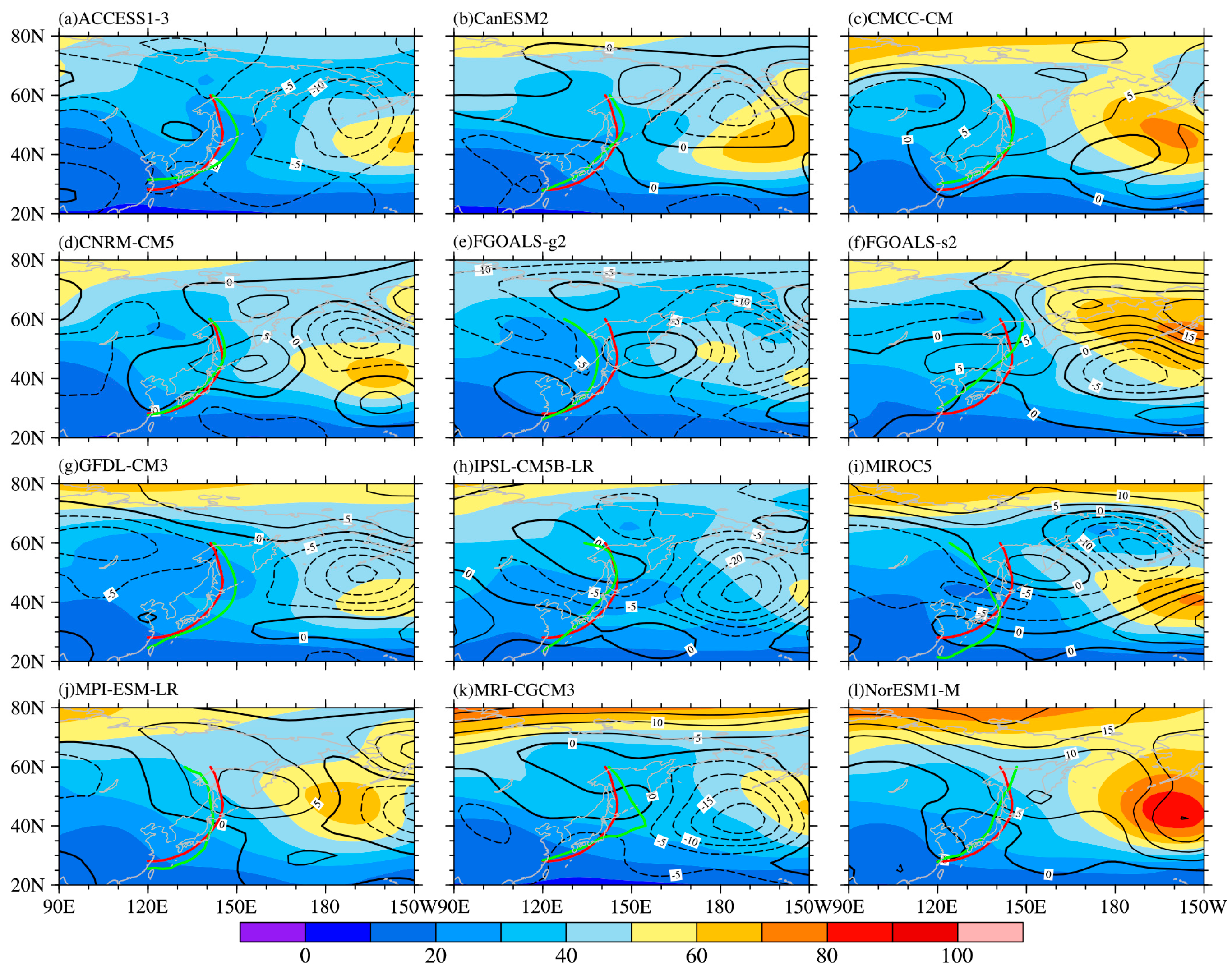
3.1. Climatological Characteristics of the EAT

The EAT is an important component of the EAWM and its main activity region is located over 120°–160° E [27]. Figure 1a shows the climatology of the geopotential height at 500 hPa in the observations. It is clear that the EAT lies over East Asia and the adjacent sea. The trough line of EAT (the zero isoline of gradients of geopotential height at 500 hPa in latitudinal direction) is to the east of the Japanese Islands and extends from the Sea of Okhotsk to the East China Sea along the Karafuto and Japanese archipelagos. The MME of the 12 CMIP5 models reproduces reasonably well the features of EAT (Figure 1b) but the geopotential height is lower than the observations (negative biases), especially over the southern EAT region. The trough line in the MME also extends from the Sea of Okhotsk to the East China Sea but is slightly farther west than that in the observations. The interannual variability of the geopotential height at 500 hPa is not prominent over the EAT region; the strongest interannual variability is over the Northeastern Pacific to the east of EAT (Figure 1c). In the MME, the interannual variations of the geopotential height at 500 hPa are much weaker than in the observations (Figure 1d), which indicates that the MME underestimates the interannual variability of the EAT.

Although the MME can reproduce the EAT successfully, the simulated EAT varies with the model. The climatology and interannual standard deviations of the geopotential height at 500 hPa in individual CMIP5 models are shown in Figure 2 and Figure 3, respectively. All the models used in this study can reproduce the EAT over East Asia as in the observations. However, the intensity, trough line, and interannual variability of the EAT simulated in CMIP5 models show prominent biases compared with the observations. In most CMIP5 models (CanESM2, CNRM-CM5, FGOALS-g2, GFDL-CM3, IPSL-CM5B-LR, and MRI-CGCM3), the geopotential height shows negative biases over the EAT region. In the MIROC5 and NorESM1-M, the geopotential height is enhanced over the northern EAT and weakened over the southern EAT. In the FGOALS-s2, the geopotential height is enhanced over the southern EAT and weakened over the northern EAT. In the ACCESS1-3, GFDL-CM3, and MRI-CGCM3, the trough line is to the east of that in the observations. The location of the trough line deviates considerably from the observations in the FGOALS-g2, FGOALS-s2, MIROC5, and MRI-CGCM3 models. The trough line is much farther west in FGOALS-g2 and MIROC5 than in the observations over the northern EAT. All of the models can capture the relatively weak interannual variability over the EAT region compared with that over the Northeastern Pacific. In ACCESS1-3, GFDL-CM3, and FGOALS-g2, the interannual variability of EAT is weaker than the observations. In contrast, in CMCC-CM, CNRM-CM5, FGOALS-s2, and NorESM1-M, it is stronger, especially over the northern EAT.

To show the similarities and differences between the observations and 12 CMIP5 models more clearly, Taylor diagrams for the climatology and interannual standard deviation of the geopotential height over the EAT region (25°–70° N, 100°–180° E) are shown in Figure 4. All of the models show high pattern correlations with the observations for the climatology of geopotential height. The corresponding correlation coefficients exceed 0.95 for all 12 CMIP5 models and the spatial variations of the climatological mean are close to the observations. The intermodel spreads of climatology in the 12 CMIP5 models are shown in Figure 5a. The intermodel spreads of climatology are smaller over the northern part of EAT than over the southern part, which means that the simulated EAT varies considerably among the models over the southern part. The pattern correlation of interannual standard deviation between CMIP5 models and observations is lower than that of the climatological intensity over the EAT region (Figure 4b) with pattern correlation coefficients below 0.9 in half the models, indicating poorer performances than for the climatology. The main biases are over the Northeastern Pacific (Figure 3). The interannual variability is underestimated over the Northeastern Pacific in more than half the models, which results in the low pattern correlation coefficients and large biases in normalized standardized deviations in Figure 4b. The intermodel spreads of interannual variability in CMIP5 models are shown in Figure 5b. The simulated interannual variability varies considerably over the northern part of EAT and the Northeastern Pacific.

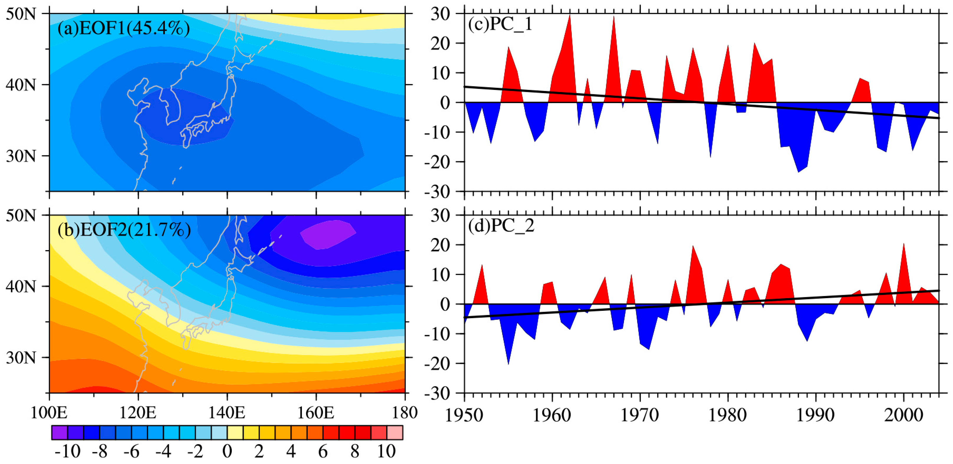
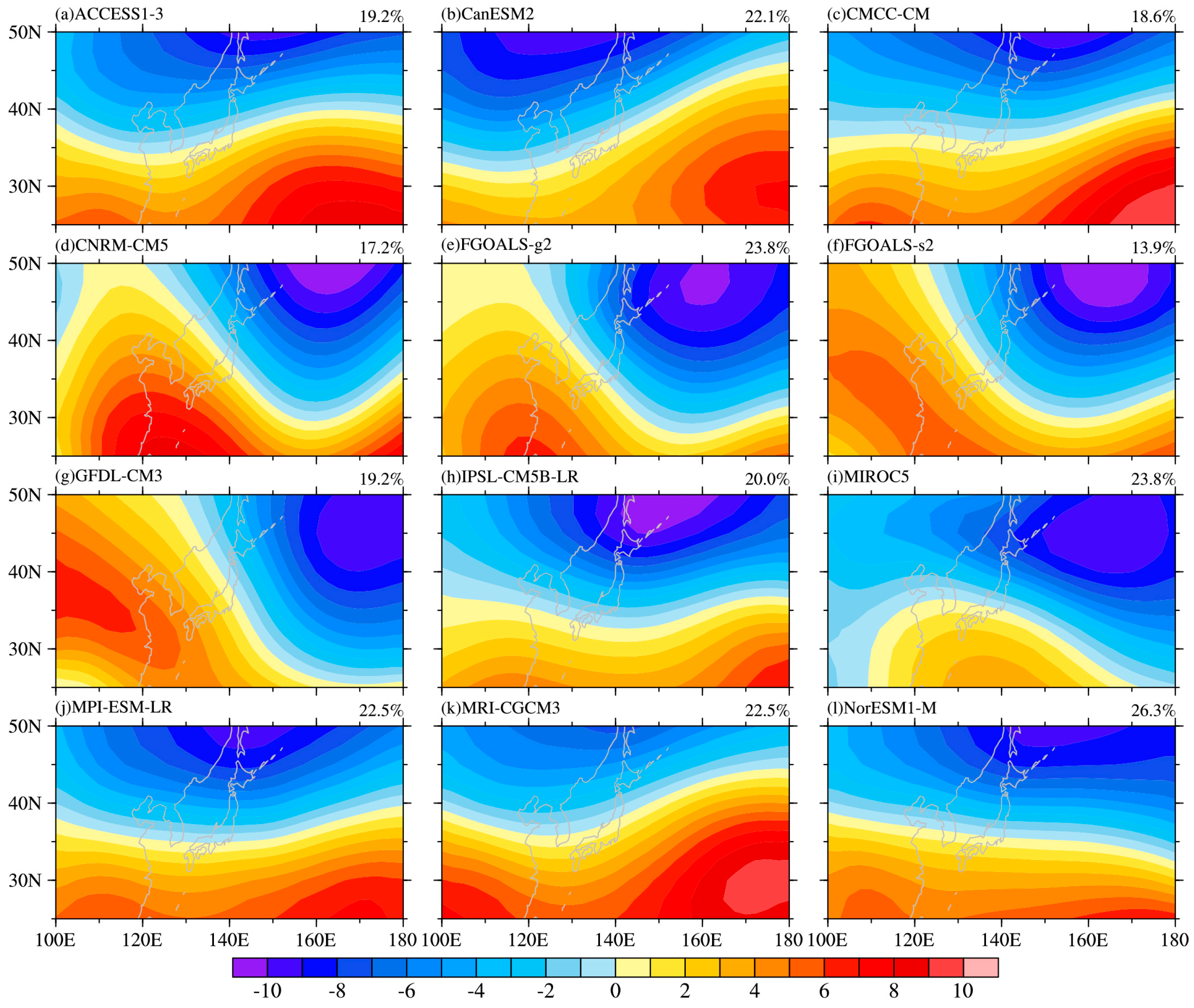
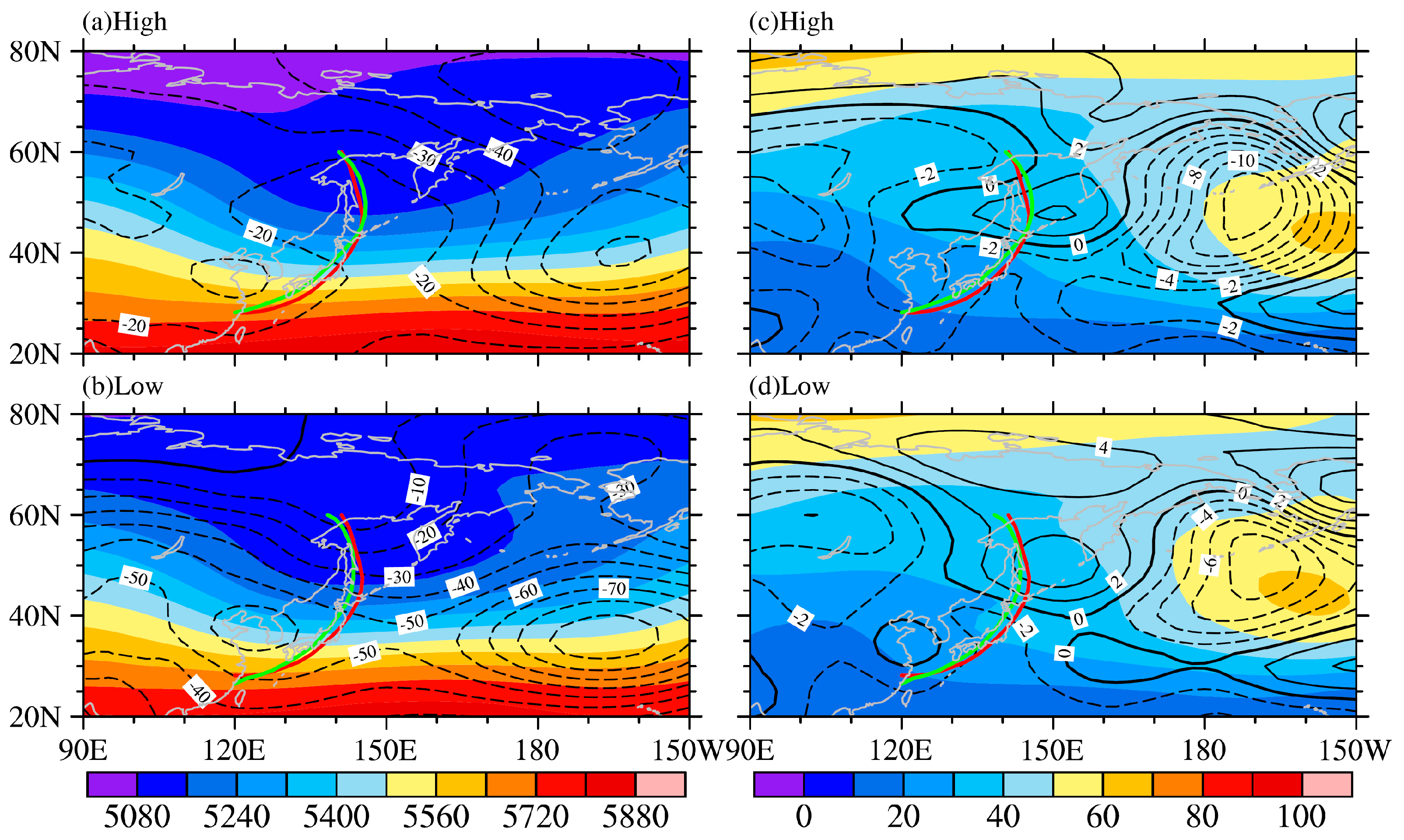
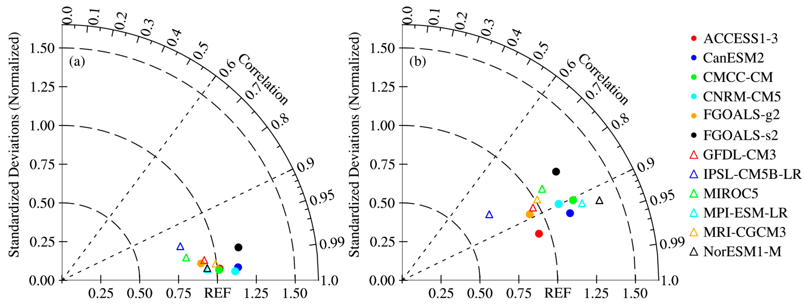
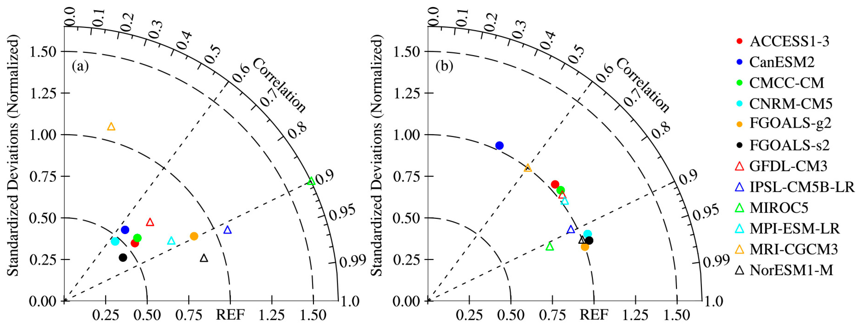
3.2. Spatial Modes of EAT Activity

The EAT activity has two prominent modes, as indicated by Wang et al. [1], which can be represented by the first two EOF modes of the standardized geopotential height at 500 hPa over 25°–50° N, 100°–180° E in the boreal winter. Figure 6 shows the first two EOF modes and corresponding time series in observations. The first EOF mode indicates the coherent variations of the geopotential height over the EAT region, which reflects the intensity variations of EAT and the activity of EAWM. The activity center of the first EOF mode is over the Korean Peninsula and Japanese Islands. The time series of the first EOF mode shows a significant linear weakening trend. The second EOF mode exhibits a north–south seesaw pattern, which reflects the variations of the EAT axis and the path of EAWM cold surge. The two activity centers of the second EOF mode are around 48° N, 160° E and 25° N, 110° E, respectively. In winters with a weak second EOF mode, the meridional circulation is enhanced and the slope of the trough line is lower [1]. The time series of the second EOF mode shows a significant linear strengthening trend. Therefore, it is important to investigate the nature of the two modes in the 12 CMIP5 models.

The first EOF modes in individual CMIP5 models are shown in Figure 7. Although the first mode reflects the coherent variations in the geopotential height over East Asia in all 12 CMIP5 models, there are many biases compared with the observations. About half the models underestimate the intensity of this mode and only one model (MRI-CGCM3) overestimates its intensity. Seven out of the 12 CMIP5 models cannot capture the activity center of this mode over the Korean Peninsula and Japanese Islands; the activity center is to the east of the Japanese Islands in FGOALS-s2, IPSL-CM5B-LR, MPI-ESM-LR, and NorESM1-M. The linear trend of the time series of the first EOF mode in CMIP5 models is listed in

Table 2. Linear trend of the empirical orthogonal function (EOF) mode time series in the observations and CMIP5 models. “*” denotes the results exceeding the significant test at 90% confidence level, unit: /10a.

Models	PC1	PC2
Observations	−1.955 *	1.671 *
ACCESS1-3	0.040	−0.002
CanESM2	−1.275	−0.831
CMCC-CM	−3.725 *	0.425
CNRM-CM5	−0.350	0.296
FGOALS-g2	−2.483 *	0.244
FGOALS-s2	−5.730 *	0.301
GFDL-CM3	0.066	0.248
IPSL-CM5B-LR	−2.436 *	1.401 *
MIROC5	−0.825	1.199
MPI-ESM-LR	−3.430 *	1.152
MRI-CGCM3	−1.720 *	−0.755
NorESM1-M	−1.589	−0.290

. Apart from ACCCESS1-3 and GFDL-CM3, the models capture the linear weakening trend of the first EOF mode seen in the observations, and in five models (CMCC-CM, FGOALS-s2, FGOALS-g2, IPSL-CM5B-LR, and MPI-ESM-LR) this linear weakening trend is overestimated. The Taylor diagram for the first EOF mode in the CMIP5 models is shown in Figure 8a. Only three models (MIROC5, IPSL-CM5B-LR, and NorESM1-M) have pattern correlation coefficients exceeding 0.9, and more than half of the models yield pattern correlation coefficients between 0.6 and 0.9. The normalized standardized deviations show large biases compared with the observations, which means that the spatial standard deviation of the first EOF mode is not well captured in the CMIP5 models. Ten out of the twelve CMIP5 models underestimate the spatial standard deviation, which mainly results from the underestimated intensity and the shifted activity center of the first EOF mode. The lowest pattern correlation coefficient is observed in the MRI-CGCM3 model, which is induced by the overestimated intensity and eastward shifted activity center of the first EOF mode (Figure 7k).

The second EOF modes in the 12 CMIP5 models are shown in Figure 9. More than half the models can reproduce the north–south seesaw variations as in the observations. However, all the models fail in simulating the location of the two activity centers of this mode. In four models (CNRM-CM5, FGOALS-g2, FGOALS-s2, and GFDL-CM3), the second EOF mode mainly shows east–west rather than north–south seesaw variations. The Taylor diagram for the second EOF mode in CMIP5 models is shown in Figure 8b. Only five models have pattern correlation coefficients exceeding 0.9. The normalized standardized deviations of the second EOF modes are close to the observations, which means that the spatial standard deviation of the second EOF mode in CMIP5 models is comparable to that in the observations. The linear trend of the time series of the second EOF mode in each CMIP5 models is listed in Table 2. Eight out of the 12 CMIP5 models reproduce the linear strengthening trend but all the simulated linear strengthening trends are weaker than in the observations. In the other four models (ACCESS1-3, CanESM2, MRI-CGCM3, and NorESM1-M), the time series of the second EOF mode shows a linear weakening trend, opposite to the observations.

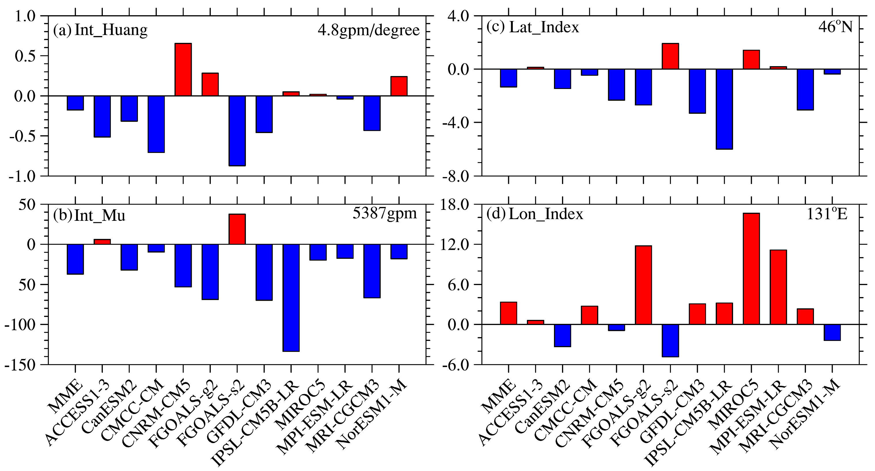
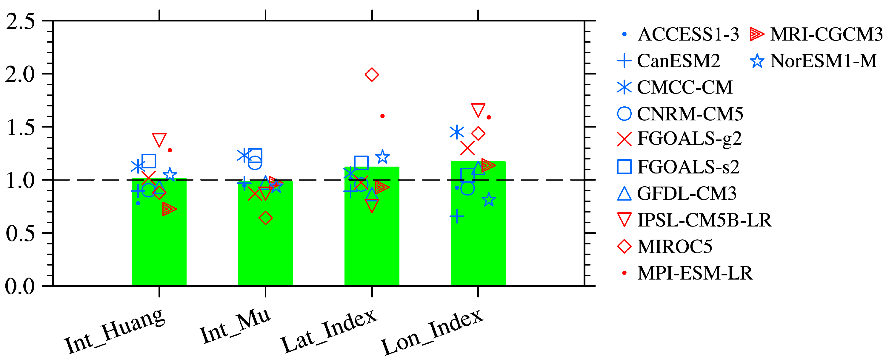
3.3. Characteristic Indices Related to the EAT

The analyses above explored the spatial characteristics of the EAT simulated in the CMIP5 models. In the following, we investigate the activity of the EAT based on its characteristic indices: the dynamic intensity index, the static intensity index, the latitude index, and the longitude index. The dynamic intensity index of the EAT is defined by Huang [27] (referred to as Int_Huang):

$$Int\_Huang=-\frac{\mathsf{\Phi }({\lambda }_2)-\mathsf{\Phi }({\lambda }_1)}{{\lambda }_2-{\lambda }_1}$$

(1)

where Φ(λ₂) is the minimum geopotential height at 45° N at longitude λ₂ between 120° E to 160° E; and Φ(λ₁) is the maximum geopotential height at 45° N at longitude λ₁ between 70° E to 100° E. The static intensity index of EAT is defined as the anomalous geopotential height at 500 hPa averaged over 30°–50° N, 120°–150° E [28] (referred to as Int_Mu). The latitude index of EAT is defined as the southern-most point of the 5240 gpm isoline of geopotential height at 500 hPa averaged over 120°–160° E (referred to as Lat_Index). The longitude index of EAT is defined by Huang [27] (referred to as Lon_Index):

$$L\mathrm{on}\text{\_}\mathrm{Index}=({\lambda }_1+{\lambda }_2)/2$$

(2)

where λ₁ (λ₂) is the longitude of the minimum geopotential height at 35° N (55° N) between 120° E and 160° E. The dynamic intensity index of EAT can reflect the intensity of anomalous northerlies over East Asia [27]. The static intensity index of EAT depicts the variations of the EAT intensity [28]. The latitude and longitude indices of EAT describe the variations of the EAT location [27].

The biases of these indices in the CMIP5 models against the observations are shown in Figure 10. The MME dynamic intensity index underestimates the intensity of EAT by about 0.2 gpm/degree. In seven (five) CMIP5 models, the dynamic intensity of EAT is underestimated (overestimated) compared with the observations. Negative (positive) biases in the dynamic intensity index mean weakened (strengthened) northerlies over East Asia [27]; therefore, the northerlies simulated in the CMIP5 models are weaker in seven of the CMIP5 models than in the observations. The MME static intensity index overestimates the intensity of EAT with a negative bias of about 35 gpm. In ten (two) CMIP5 models, the static intensity index of EAT is overestimated (underestimated) compared with the observations; in IPSL-CM5B-LR, the negative bias exceeds 130 gpm. The climatological value of the latitude index of EAT is about 46° N in the observations; there are negative biases in the MME and eight CMIP5 models and positive biases in four CMIP5 models. These results indicate that the simulated EAT lies farther south than in the observations in more than half of the models. The climatological of longitude index of EAT is about 131° E in the observations, and there are positive biases in MME and eight CMIP5 models and negative biases in four CMIP5 models. These results imply that the simulated EAT in most CMIP5 models is farther east than in the observations.

The ratios of the interannual variability of the four EAT characteristic indices between the observations and the CMIP5 models are shown in Figure 11. The variability of the dynamic and static intensity indices in MME is almost identical to that in the observations and about half the models capture this feature very well. However, the variability of the MME latitude and longitude indices is greater than in the observations, especially that of the longitude index. The intermodel spreads in the interannual variability of these four EAT-related parameters are larger for the latitude and longitude indices and smaller for the dynamic and static intensity indices. These results imply that the CMIP5 models perform better in simulating EAT intensity than location.

3.4. Effects of Model Resolution

The performances of the CMIP5 models in simulating EAT varies with the model, which gives rise to the question of whether this is related to model resolution. The 12 CMIP5 models were divided into two groups: the high-resolution group (the grid-points are greater than 100 in both directions) and the low-resolution group (the grid-points are less than 100 in one or both directions). Figure 12 shows the climatological mean of the geopotential height at 500 hPa and its interannual standard deviations for the high- and low-resolution models. The anomalous geopotential height is negative both in high and low-resolution models. The interannual standard deviations simulated in CMIP5 models are greater over the northern part of the EAT and weaker over the southern part than in the observations for both the high- and low-resolution models. The climatological mean and interannual standard deviations of the EAT characteristic indices are also composited for the two groups (

Table 3. Composited differences of EAT characteristic indices and the ratios of interannual standard deviation in high- and low-resolution models.

Index	Climatological Mean		Ratios of Interannual Standard Deviation
High/Low group	High	Low	High	Low
Int_Huang	−0.229	−0.136	1.013	1.098
Int_Mu	−19.27	−49.98	0.981	0.974
Lat_Index	−0.382	−2.013	1.119	1.054
Lon_Index	2.755	3.737	1.171	1.227

). The differences in Int_Mu, Lat_Index, and Lon_index (Int_Huang) are smaller in the high (low)-resolution models. The interannual standard deviations of Int_Huang and Lon_Index (Int_Mu and Lat_Index) are closer to the observations in the high (low)-resolution cases. The spatial pattern of EAT simulated in CMIP5 models is not closely related to the resolution of the models. The spatial correlation coefficient of interannual standard deviation in FGOALS-s2 (high-resolution model) is lower than in CanESM2 (low-resolution model) and is greater in ACCESS1-3 (high-resolution model) than in IPSL-CM5B-LR (low-resolution model). Therefore, the horizontal resolution of CMIP5 models is not closely related to their performances in simulating the activity of EAT.

4. Conclusions

Based on the NCEP reanalysis data and the output of 12 CMIP5 models, this study has evaluated the performance of CMIP5 models in simulating the climatology and interannual variability of the EAT. The main conclusions are as follows.

In the climatological mean sense, the 12 CMIP5 models can successfully reproduce the intensity and spatial distributions of the geopotential height at 500 hPa over the EAT region. The prominent intermodel spreads of the geopotential height at 500 hPa occur over the southern part of EAT. The dynamic intensity of the EAT is underestimated by most CMIP5 models but the static intensity is stronger in most models than in the observations, which may result from the negative biases of the geopotential height in the CMIP5 models. The latitude of EAT simulated in MME is about 1.5° south of the observations and the longitude of EAT simulated in MME is about 3° east of the observations. The interannual variability of the geopotential height at 500 hPa is greater over the northern EAT than over the southern EAT and this is successfully reproduced in all CMIP5 models. However, the interannual variability in MME is weaker than in the observations. The CMIP5 models simulate the interannual variability of the geopotential height at 500 hPa less well than the climatological intensity. The magnitude of the interannual variability of EAT intensity simulated in the CMIP5 models is almost identical to the observations, especially in the MME. However, the magnitude of the interannual variability of EAT latitude and longitude locations is greater than in the observations and the intermodel spreads among the 12 CMIP5 models are also larger.

The coherent variation mode of the geopotential height over East Asia can be reproduced in all 12 CMIP5 models but the intensity and location of its activity center are only successfully captured in half of the models. Only MRI-CGCM3 simulates an intensity stronger than the observations. The linear weakening trend of this mode is simulated in ten out of the twelve CMIP5 models and it is stronger in five models than in the observations. The north–south seesaw variations of the geopotential height over the EAT regions are reproduced in eight out of the twelve CMIP5 models, but none of the models capture its two activity centers correctly. The linear strengthening trend of this mode is observed in eight out of the twelve CMIP5 models but its intensity is much weaker than in the observations. Four models cannot reproduce the second EOF mode of EAT; the reasons are unknown and need further investigation. The horizontal resolution of the CMIP5 models is not closely related to their performances in simulating the EAT. The linear trends of the two leading EOF mode time series have also been investigated with other reanalysis datasets: JRA-55 [29], ERA-40 [30] and 20CR-V2c [31]. The linear decreasing trend of the first EOF mode time series and increasing trend of the second EOF mode time series are also detected in these three reanalysis datasets, which indicates that the variation in the linear trend among the four reanalysis datasets is consistent. However, only the linear decreasing trend of the first EOF mode time series in JRA-55 is significant at the 90% confidence level, which means that the significance of the linear trend may depend on the reanalysis data. Therefore, the results of this study are repeatable and reliable using NCEP reanalysis data but should be used with caution, especially when using other reanalysis data.

References

1. Wang, L.; Chen, W.; Zhou, W.; Huang, R.H. Interannual variations of 500 hPa East Asian trough axis and its association with the East Asian winter monsoon pathway. J. Clim. 2009, 22, 600–614. [Google Scholar] [CrossRef]
2. Huang, R.H.; Chen, J.L.; Wang, L.; Li, Z.D. Characteristics, processes, and causes of the spatio-temporal variabilities of the East Asian monsoon system. Adv. Atmos. Sci. 2012, 29, 910–942. [Google Scholar] [CrossRef]
3. Academia Sinica. On the general circulation over eastern Asia. Part I. Tellus 1957, 9, 432–446. [Google Scholar]
4. Ye, D.Z.; Zhu, B.Z. Several Problems of Atmospheric Circulation; Science Press: Beijing, China, 1958. (In Chinese) [Google Scholar]
5. Boyle, J.S.; Chen, T.J. Synoptic aspects of the wintertime East Asian monsoon. In Monsoon Meteorology; Chang, C.P., Krishnamurti, T.N., Eds.; Oxford University Press: Oxford, UK, 1987; pp. 125–160. [Google Scholar]
6. Lau, K.M.; Li, M.T. The monsoon of East Asia and its global associations—A survey. Bull. Am. Meteorol. Soc. 1984, 65, 114–125. [Google Scholar] [CrossRef]
7. Ding, Y.H. Monsoon over China; Kluwer Academic Publishers: Boston, CA, USA, 1994. [Google Scholar]
8. Zhou, W.; Chan, J.C.L.; Chen, W.; Ling, J.; Pinto, J.G.; Shao, Y.P. Synoptic-scale controls of persistent low temperature and icy weather over southern China in January 2008. Mon. Weather Rev. 2009, 137, 3978–3991. [Google Scholar] [CrossRef]
9. Chang, C.P.; Lau, K.M. Northeasterly cold surges and neat-equatorial disturbances over the winter MONEX area during December 1974. Part II: Planetary-scale aspects. Mon. Weather Rev. 1980, 108, 298–312. [Google Scholar] [CrossRef]
10. Zeng, H.L.; Gao, X.Q.; Dai, X.G. Analysis on interdecadal change characteristics of global winter and summer sea surface pressure field and 500 hPa height field in recent twenty years. Plateau Meteorol. 2002, 21, 66–73. (In Chinese) [Google Scholar]
11. Li, F.; Jiao, H.Y.; Ding, Y.H.; Jin, R.H. Climate change of Arctic atmospheric circulation in last 30 years and its effect on strong cold events in China. Plateau Meteorol. 2006, 25, 209–219. (In Chinese) [Google Scholar]
12. Gong, D.Y.; Wang, S.W.; Zhu, J.H. East Asian winter monsoon and Arctic Oscillation. Geophys. Res. Lett. 2001, 28, 2073–2076. [Google Scholar] [CrossRef]
13. Li, C.Y. The frequent activity of East Asian trough and the occurrence of El Niño. Sci. China 1988, 18, 667–674. (In Chinese) [Google Scholar]
14. Li, C.Y. Interaction between anomalous winter monsoon in East Asia and El Niño events. Adv. Atmos. Sci. 1990, 7, 36–46. [Google Scholar]
15. Xu, J.; Chan, J.C.L. The role of the Asian-Australian monsoon system in the onset time of El Niño events. J. Clim. 2001, 14, 418–433. [Google Scholar] [CrossRef]
16. Chang, C.P.; Lau, K.M. Short-term planetary-scales interactions over the tropics and midlatitudes during northern winter. Part I: Contrasts between active and inactive periods. Mon. Weather Rev. 1982, 110, 933–946. [Google Scholar] [CrossRef]
17. Ji, L.R.; Sun, S.Q.; Arpe, K.; Bengtsson, L. Model study on the interannual variability of Asian winter monsoon and its influence. Adv. Atmos. Sci. 1997, 14, 1–22. [Google Scholar]
18. Li, C.Y.; Mu, M.Q.; Bi, X.Q. Inter-decadal Variations of Atmospheric Circulation Part II: GCM Simulation Study. Chin. J. Atmos. Sci. 2000, 24, 739–748. (In Chinese) [Google Scholar]
19. He, S.P.; Wang, H.J. Analysis of the decadal and interdecadal variations of the East Asian winter monsoon as simulated by 20 coupled models in IPCC AR4. Acta Meteorol. Sin. 2012, 26, 476–488. [Google Scholar] [CrossRef]
20. Kimoto, M. Simulated change of the East Asia circulation under global warming scenario. Geophys. Res. Lett. 2005, 32, L16701. [Google Scholar] [CrossRef]
21. Hu, Z.Z.; Bengtsson, L.; Arpe, K. Impact of global warming on the Asian winter monsoon in a coupled GCM. J. Geophys. Res. 2000, 105, 4607–4624. [Google Scholar] [CrossRef]
22. Xu, M.M.; Xu, H.M.; Ma, J. Responses of the East Asian winter Monsoon on global warming in CMIP5 models. Int. J. Climatol. 2016, 36, 2139–2155. [Google Scholar] [CrossRef]
23. Wei, K.; Xu, T.; Du, Z.C.; Gong, H.N.; Xie, B.H. How well do the current state-of-the-art CMIP5 models characterise the climatology of the East Asian winter monsoon? Clim. Dyn. 2014, 43, 1241–1255. [Google Scholar] [CrossRef]
24. Gong, H.N.; Wang, L.; Chen, W.; Wu, R.G.; Wei, K. The climatology and interannual variability of the East Asian winter monsoon in CMIP5 models. J. Clim. 2014, 17, 1659–1678. [Google Scholar] [CrossRef]
25. Hong, J.Y.; Ahn, J.B.; Jhun, J.G. Winter climate changes over East Asian region under RCP scenarios using East Asian winter monsoon indices. Clim. Dyn. 2017, 48, 577–595. [Google Scholar] [CrossRef]
26. Kalnay, E.; Kanamitsu, M.; Kistler, R.; Collins, W.; Deaven, D.; Gandin, L.; Iredell, M.; Saha, S.; White, G.; Woollen, J.; et al. The NCEP/NCAR 40-year reanalysis project. Bull. Am. Meteorol. Soc. 1996, 77, 437–471. [Google Scholar] [CrossRef]
27. Huang, X.M. A Further Look at the Interannual Variations of East Asian Trough and Their Impacts on Winter Climate of China. Master’s Thesis, Nanjing University of Information Science and Technology, Nanjing, China, 2013. [Google Scholar]
28. Mu, M.Q.; Li, C.Y. Interdecadal Variations of Atmospheric Circulation I. Observational Analyses. Clim. Environ. Res. 2000, 5, 233–241. (In Chinese) [Google Scholar]
29. Kobayashi, S.; Ota, Y.; Harada, Y.; Ebita, A.; Moriya, M.; Onoda, H.; Onogi, K.; Kamahori, H.; Kobayashi, C.; Endo, H.; et al. The JRA-55 Reanalysis: General specifications and basic characteristics. J. Meteorol. Soc. Jpn. 2005, 93, 5–48. [Google Scholar] [CrossRef]
30. Uppala, S.M.; Kållberg, P.W.; Simmons, A.J.; Andrae, U.; Da Costa Bechtold, V.; Fiorino, M.; Gibson, J.K.; Haseler, J.; Hernandez, A.; Kelly, G.A.; et al. The ERA-40 Re-Analysis. Q. J. R. Meteorol. Soc. 2005, 131, 2961–3012. [Google Scholar] [CrossRef]
31. Compo, G.P.; Whitaker, J.S.; Sardeshmukh, P.D. The Twentieth Century Reanalysis Project. Q. J. R. Meteorol. Soc. 2011, 137, 1–28. [Google Scholar] [CrossRef]
Figure 1. (a) Climatological mean of the geopotential height at 500 hPa and (c) its interannual standard deviations in the boreal winter based on observations (unit: gpm); (b,d) As in (a,c) but for the multimodel ensemble (MME) of the 12 CMIP5 (Coupled Model Intercomparison Project phase 5) models. The contours in (b,d) denote the differences between observations and MME. The red (green) lines represent the trough line in the observations (MME).
Atmosphere 09 00067 g001
Figure 2. Climatological mean of the geopotential height at 500 hPa in individual CMIP5 models (colors, gpm) and its difference from the observations (contours, interval is 20 gpm). The red (green) lines represent the trough line in the observations (individual CMIP5 models). (al) represent different CMIP5 models as indicated at top left in each panel.
Atmosphere 09 00067 g002
Figure 3. Interannual standard deviation of the geopotential height at 500 hPa in the boreal winter for individual CMIP5 models (colors, gpm) and its difference from the observations (contours, interval is 5 gpm). The red (green) lines represent the trough line in the observations (individual CMIP5 models). (al) represent different CMIP5 models as indicated at top left in each panel.
Atmosphere 09 00067 g003
Figure 4. Taylor diagrams of (a) the climatological mean and (b) the interannual standard deviation of the geopotential height at 500 hPa over 25°–70° N, 100°–180° E in the boreal winter.
Atmosphere 09 00067 g004
Figure 5. (a) Climatological mean of the geopotential height at 500 hPa in the MME (colors, gpm) and their intermodel spreads (contours, shown as the standard deviation among 12 CMIP5 models); (b) as in (a), but for the interannual standard deviation in the boreal winter. Red line represents the EAT trough line in MME.
Atmosphere 09 00067 g005
Figure 6. (a) First and (b) second empirical orthogonal function (EOF) modes of the geopotential height at 500 hPa in the observations and (c,d) their time series. The lines in (c,d) indicate the linear trends.
Atmosphere 09 00067 g006
Figure 7. First EOF mode of the geopotential height at 500 hPa in individual CMIP5 models and their variance contribution (top right in each panel). (al) represent different CMIP5 models as indicated at top left in each panel.
Atmosphere 09 00067 g007
Figure 8. Taylor diagrams for the (a) first and (b) second EOF modes.
Atmosphere 09 00067 g008
Figure 9. As in Figure 7, but for the second EOF mode. (al) represent different CMIP5 models as indicated at top left in each panel.
Atmosphere 09 00067 g009
Figure 10. Differences in the long-term mean EAT-related parameters between the CMIP5 models and observations. (a) the dynamic intensity index, (b) the static intensity index, (c) the latitude index, and (d) the longitude index. The climatological mean in observations is presented at the top right in each panel.
Atmosphere 09 00067 g010
Figure 11. Ratios of the interannual standard deviation of EAT-related parameters in 12 CMIP5 models to that in the observations. Symbols (green bars) indicate the results of individual CMIP5 models (the MME).
Atmosphere 09 00067 g011
Figure 12. (a,b) Climatological mean of the geopotential height at 500 hPa and (c,d) its interannual standard deviation composited in (a,c) high and (b,d) low resolution CMIP5 models. The contours indicate their differences with respect to observations. The red (green) lines represent the trough line in the observations (high/low-resolution CMIP5 models).
Atmosphere 09 00067 g012