Linear or Nonlinear Modeling for ENSO Dynamics?


1
ISMAR-CNR, 19032 La Spezia, Italy
2
NOAA-ESRL, Physical Sciences Division, University of Colorado, CIRES, Boulder, CO 80305, USA
3
Physics Department, Pisa University, 56127 Pisa, Italy
*
Author to whom correspondence should be addressed.
Atmosphere 2018, 9(11), 435; https://doi.org/10.3390/atmos9110435
Submission received: 12 September 2018
/
Revised: 31 October 2018
/
Accepted: 4 November 2018
/
Published: 8 November 2018
(This article belongs to the Special Issue El Niño Southern Oscillation (ENSO))
Abstract
:The observed ENSO statistics exhibits a non-Gaussian behavior, which is indicative of the presence of nonlinear processes. In this paper, we use the Recharge Oscillator Model (ROM), a largely used Low-Order Model (LOM) of ENSO, as well as methodologies borrowed from the field of statistical mechanics to identify which aspects of the system may give rise to nonlinearities that are consistent with the observed ENSO statistics. In particular, we are interested in understanding whether the nonlinearities reside in the system dynamics or in the fast atmospheric forcing. Our results indicate that one important dynamical nonlinearity often introduced in the ROM cannot justify a non-Gaussian system behavior, while the nonlinearity in the atmospheric forcing can instead produce a statistics similar to the observed. The implications of the non-Gaussian character of ENSO statistics for the frequency of extreme El Niño events is then examined.
1. Non-Gaussian-Nonlinear Features of the ENSO Statistics
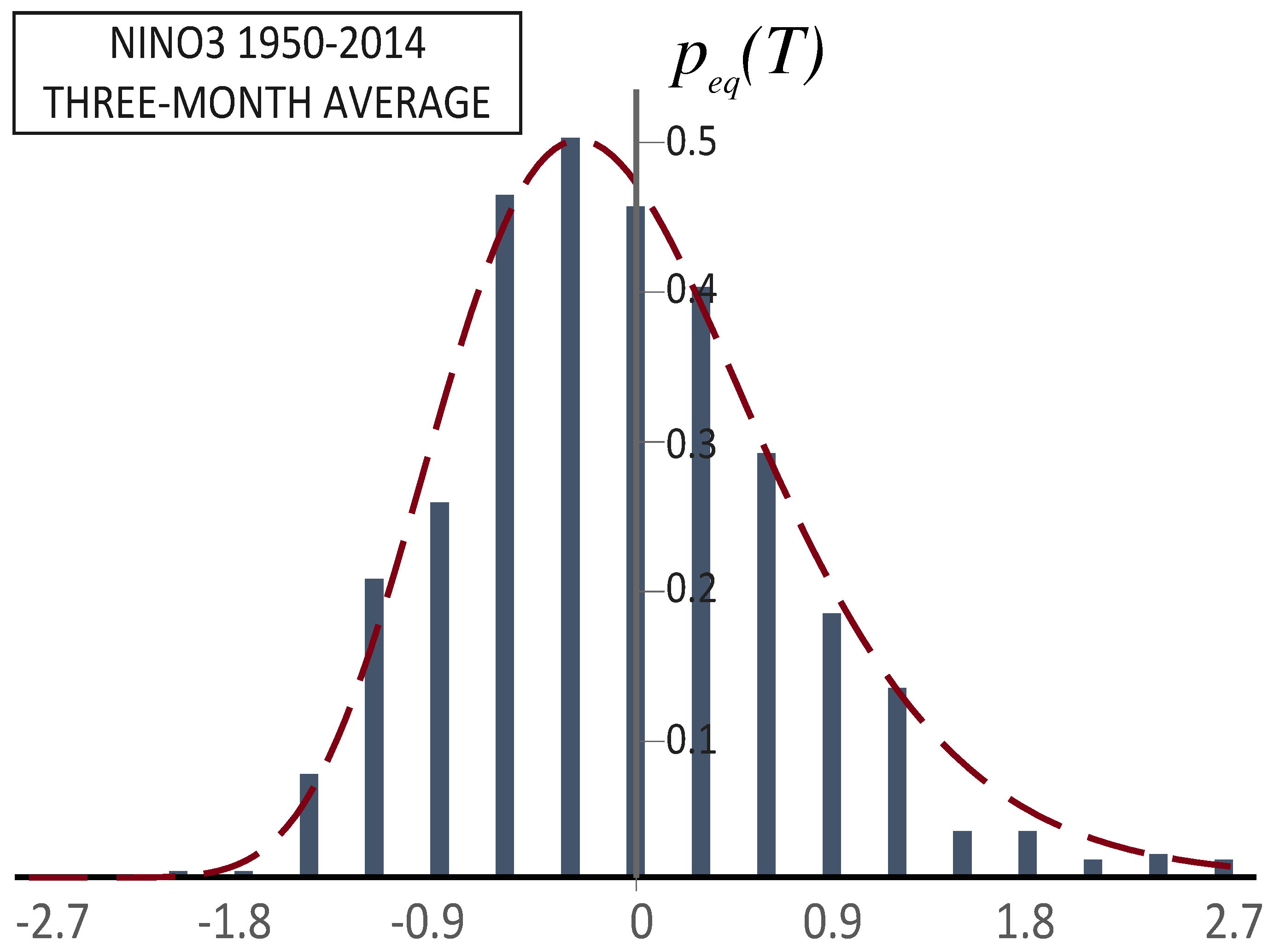
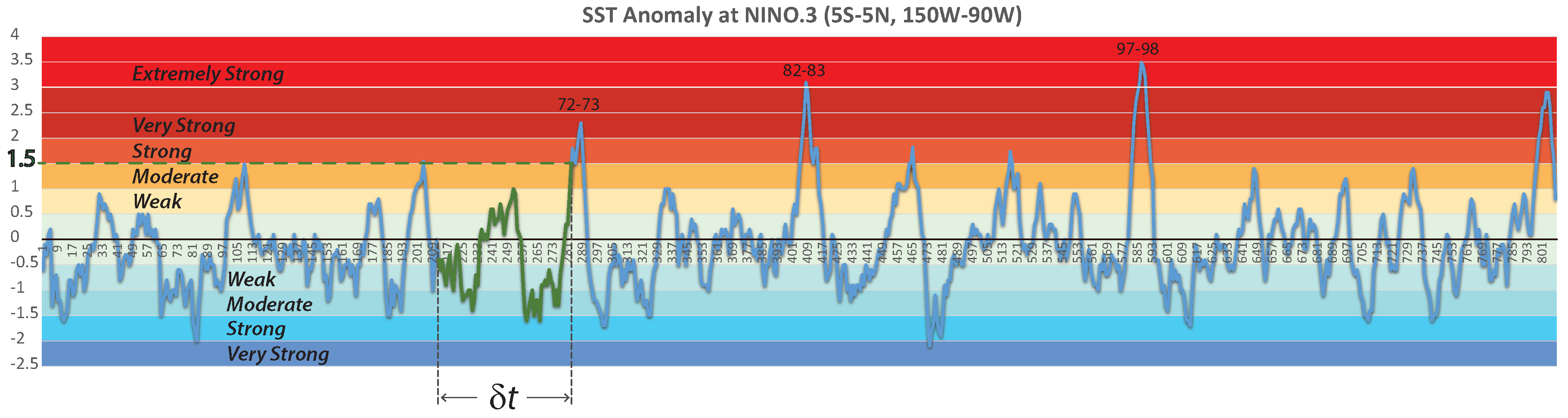
It is well established that some aspects of the El Niño Southern Oscillation (ENSO) have a non-Gaussian statistics, a characteristic that is indicative of some underlying nonlinear process. For example, the plot of the frequency of the Niño 3 index (averaged Sea Surface Temperature (SST) anomalies in the region S– N, W– W) shows that the likelihood of large positive SST anomalies is greater than that of negative anomalies (Figure 1), indicating that the SST anomalies achieved in the eastern equatorial Pacific during the mature phase of an El Niño are larger than those occurring during la Niña events. Another asymmetry is the duration of the transition from one ENSO phase to the other, with a rapid transition from El Niño to La Niña, but a slower transition from La Niña to El Niño [1]. The duration of El Niño events tends to be shorter than that of La Niña ones, and the range of El Niño flavors is larger than that of La Niña [2].
This non-Gaussian behavior is quantified by the positive skewness of the SST distribution: . A positive kurtosis also clearly indicates that extreme events are more likely to occur than for a normal distribution.
The non-Gaussianity of the histogram arises from non-linear contributions in the equation of motion governing the system, and it is important to understand which nonlinearities play the most relevant role in the ENSO evolution. We know that ENSO is the result of complex large-scale ocean-atmosphere interactions that also include non-linear processes. For instance, An and Jin [3] proposed that the Nonlinear Dynamical Heating (NDH) in the ocean mixed layer is crucial for generating intense El Niño events, mainly due to the vertical nonlinear advection. Asymmetries in intensity can also result from ocean-atmosphere coupling processes (e.g., [4]) or from the nonlinear response of the zonal wind stress to ENSO SST anomalies [5,6]. In general, the complexity of the ENSO, as for most of the large-scale phenomena resulting from the ocean-atmosphere interaction, makes it challenging to understand the general key features of the statistics and dynamics of the events. Thus, to mimic the highly complex nature of ENSO events, as the diversity in spatial flavors and the “non-normal” growth of fluctuations [7], large multivariate linear models with multivariate additive stochastic perturbations have been exploited [8,9]. Here, we focus instead on Low Order Models (LOMs), i.e., the set of Ordinary Differential Equations (ODE) for ENSO, perturbed by a fast and chaotic forcing. Probably, a more realistic modeling of ENSO should merge these two pictures (multidimensionality and nonlinearities). A deeper discussion about the effective and respective roles of the dimension and of the nonlinearities of an LOM to model the complexity of ENSO goes beyond the task of the present work.
The tropical Pacific can be well described by shallow water equations driven at the surface by the easterly trade winds, thus allowing for a drastic simplification of the system dynamics.
Simple shallow water equations together with the assumption of a large timescale separation between the ENSO dynamics and the typical dynamics of atmospheric processes make it possible to reduce the description of the dynamics of the ENSO-relevant variables, to a relatively simple LOM. This LOM can be separated in a slow part, or “system of interest”, associated with the slow evolution of oceanic variables like SST and thermocline depth, and a fast “rest of the system” that primarily includes fast atmospheric processes, e.g., the Madden–Julian Oscillation (MJO), the Westerly Wind Bursts (WWBs), etc., which are considered important in forcing ENSO. ENSO LOMs that have been extensively considered in the literature include the Recharge Oscillator Model (ROM, e.g., [10,11,12,13,14,15,16,17] among many others) and the Delayed Oscillator (DO, e.g., [18,19]). In these models, ENSO events are triggered by the forcing provided by the fast atmospheric variables, which are usually represented as a stochastic perturbation of the system of interest.
The simplified representation of ENSO in the LOMs provides a suitable framework for examining the impact of the system nonlinearities on the ENSO statistics. In particular, an important question is whether the relevant nonlinearities reside in the interaction among the variables of the system of interest (dynamical nonlinearities), as suggested, for example in [18], or are associated with the interaction of the system of interest with the atmospheric fast forcing, as indicated, among others, by [6,20].
The fast atmospheric forcing can be included in two ways: considering this forcing as stochastic or assuming a deterministic motion with initial conditions distributed according to some distribution (the Gibbs idea of ensemble). The former approach is often used in the oceanographic field, where the dynamics is divided into a slow and a very fast and chaotic component, and the fast part is considered to be random (usually modeled as white noise) [21,22,23,24,25]. The latter approach has been largely used in the context of the foundation of statistical mechanics and thermodynamics and, more recently, also in the oceanographic field by some of the authors [17,26,27]. It aims at starting from more realistic deterministic systems (instead of the stochastic ones), and by using projection- perturbation procedures, it allows managing also the cases in which the time scale separation between the dynamics of the part of interest and that of the rest of the system is not so large: this is the reason why in this work, we shall focus on the projection-perturbation approach, which has been applied to the multi-scale ENSO system.
Both approaches have their strengths and weaknesses, and a large literature has been devoted to justify both from a formal and theoretical point of view (for a review about the foundation of the stochastic approach, see [28], and for the projection approach, see, e.g., [29,30,31,32,33]). It is far beyond the scope of the present work to discuss the foundation of these approaches. However, both aim at obtaining a Partial Differential Equation (PDE), ideally a Fokker–Planck Equation (FPE), guiding the dynamics of the Probability Density Function (PDF) for the variables of the part of interest of the system.
The FPE has been historically used to describe the PDF of Brownian-like particles [34,35]. Actually, the FPE has been recognized as a very useful tool for modeling a wide variety of stochastic phenomena arising in physics, chemistry, biology, finance, traffic flow, etc. [36]. The importance of the FPE cannot be overestimated, and in the classical books of stochastic methods, it is obtained from a truncating Kramers–Moyal expansion of the Markovian master equation [37,38,39]. From an FPE, it is possible to obtain statistical information about the quantity of interest. For example, the FPE is the major approach for determining, both analytically and numerically, important quantities like the First Passage Time (FPT; see for example [40]), in a variety of contexts ranging from civil and mechanical engineering, physical chemistry [41,42,43], disordered systems [44,45], neuroscience [46,47], biochemistry [48], biomedicine, mathematical financing, image processing, computer science, etc.
More generally, the possibility of using an FPE to model the statistical behavior of the relevant properties of the variables of interest is often crucial because the FPE is the only non-trivial partial differential equation that in many cases can be approached for a solution with analytical tools, and it looks like a Schrodinger equation [49]. In the present paper, we shall obtain a general FPE for the perturbed linear/non-linear ROM representing the ENSO dynamics, and we will compare some general statistical features resulting from the FPE (such as the stationary PDF, the relaxation properties and the average timing of the events) with observations, to infer the specific nature of the nonlinearities of the ENSO modeled by the ROM.
The contents are organized as follows: Section 2 is devoted to reviewing and discussing the way the ROM emerges as an LOM describing the dynamics of the anomalies of the thermocline depth and of the SST of the equatorial Pacific Ocean. This section shows from both a physical and observational point of view that the ROM can provide a good representation of the ENSO dynamics. In Section 3, we start discussing the nonlinearities, and we present a first result of the present paper: comparing observations with the model, it is hard to justify/detect possibly internal dynamical nonlinearities for the ROM (nonlinear coupling between the ROM variables). In Section 4, we introduce and justify the nonlinear coupling between the unperturbed ROM and the fast (but not extremely fast) forcing (mostly by the atmosphere). In Section 5, starting from the perturbed ROM, we exploit recent results [17,26,27] to obtain the explicit expression of the FPE for the ROM. This is mainly a review of previous results, but it is developed rather extensively here to make the present work self-contained. In Section 6, we use different methods (averages of first moments, covariance matrix, first passage time, power spectrum and expectation of the process time increments) to infer, from data, the values of the FPE coefficients, comparing them with the theoretical ones. The aim is to assess where the nonlinearities responsible for the non-Gaussian features of the ENSO statistics reside. Section 7 is devoted to discussing the results and drawing conclusions.
2. The Dynamics of the Components of the ENSO: The Recharge Oscillator Model
The El Niño Southern Oscillation, also known as ENSO, is a periodic fluctuation of the SST (El Niño) and the sea level pressure (Southern Oscillation) across the equatorial Pacific Ocean. The fluctuations arise over a normal condition of strong SST gradient between the east (cold tongue) and the west (warm pool) equatorial Pacific Ocean. ENSO is a complicated, not yet fully-understood, coupled ocean-atmosphere phenomenon in which basin-wide changes in sea surface temperatures, trade winds and atmospheric convection are intimately related. However, the particular ocean and atmosphere conditions that generate, and in some way also define, the El Niño/La Niña events allow the representation of the key ocean-atmospheric feedbacks responsible for this complex phenomenon in a simplified fashion.
The upper layer of the tropical Pacific Ocean, responsible for the energy and momentum exchange with the atmosphere, is a very long strip of water with a meridional width of a few hundred kilometers, a zonal extension of about 10,000 km and an average depth of about 120 m, as defined by the depth of the thermocline. The water in this strip flows over the deeper and colder ocean, from the South American coasts to the warm Asian coasts, mainly driven by the easterly trade winds and “trapped” in the convergence ocean zone, around the equatorial latitude, ultimately due to the Coriolis effect.
This motion accumulates warm water in the western Pacific Ocean, and because of the closed eastern boundary, it forces the cold and deep water to rise up in the eastern Pacific to compensate the surface water moving westward. This process generates the strong SST gradient between the two sides of the basin, which, in normal conditions, is in equilibrium with the easterly trade winds.
During an El Niño (La Niña) event, this SST gradient from east to west is reduced (increased): we consider that an El Niño (La Niña) event is occurring when the SST anomaly on the east equatorial Pacific is greater (lesser) than 0.5 (−0.5) degrees Celsius with respect to the average value. The SST anomalies are related to the thermocline depth anomalies. Thus, the key quantities that characterize ENSO in the equatorial Pacific Ocean are the SST anomaly () in the eastern part of the domain, usually described in terms of the Niño 3index (average SST in the area S– N, W– W), and the zonal average of the anomaly of the thermocline depth (h).
Exploiting these very peculiar physical conditions of the equatorial surface layer of the Pacific Ocean and from two-box (east and west side, respectively), two-strip (equatorial and off equatorial, respectively) approximations of the shallow water Navier–Stokes (NS) equations applied to the tropical Pacific Ocean, Jin obtained the following very simple system of linear equations for the Pacific equatorial thermocline depth anomaly [10,11]:
where is the zonally-integrated wind stress anomaly, the subscript W (E) means that the variables refer to the west (east) side of the basin, the friction term r collectively represents the damping of the upper ocean system through mixing and the equatorial energy loss to the boundary layer currents at the east and west sides of the ocean basin, and it is set in the range month months [10,11]. Equation (1b) describes the zonal tilt of the thermocline, which is in balance with the equatorial zonal wind stress forcing on interannual time scales (e.g., [10,51]). The Kelvin and Rossby waves, which accomplish the adjustment processes, are filtered out, in this picture, because the timescale of the mode retained in this approximation is much longer than the basin crossing time of these waves. If one assumes that for a given steady wind stress forcing, the zonal mean thermocline anomaly of this linear system is about zero at the equilibrium state, that is, (at equilibrium), then from Equation (1), one finds that shall be about half of r.
The work in [10,11] provided a physical basis for the simple linear relationships in Equation (1), in the long wave, two-strip approximation.
Notice that if the wind stress were a fast forcing completely independent of the dynamics of the thermocline depth anomaly, Equation (1) would give rise to a very simple relaxation process with relaxation time given by , which, of course, is not what happens in reality. In fact, as we shall see below, the wind dynamics has a slow part that is strongly correlated with the dynamics of h via a direct linear relationship with the other ENSO variable: the SST anomaly .
A linear ODE for the thermodynamics relationship between the variation of the anomalous SST and the thermocline depth was proposed in [10,11,52,53] and related subsequent works:
where the first term on the right-hand side is a damping process with a collective damping rate c. The second term describes the influence on of the thermocline displacement, and is the Ekman pumping coefficient of the vertical advective feedback processes due to the wind stress averaged over the domain, which actually can be considered vanishing (see [10,52,53] for details): .
Using Equation (1b), we can rewrite Equation (2) as:
The above equation relates the dynamics of to that of . However, as we have already observed, also the dynamics of , given in Equation (1), depends on the values of the variable. This dependence is due to the fact that the wind stress is strongly influenced by the zonal SST gradient. In effect, in most of the works on the ROM [52,53] and on the DO [18], it is explicitly assumed that the following linear relationship holds true:
where is a fast “chaotic” fluctuating function of time. In this work, we define as “chaotic” a unidimensional function of time if its dynamics can be considered “almost ” random so as to allow us to substitute it safely with a genuine stochastic process or to use a second-order perturbation projection approach, as hereafter specified. In the first case, we should exploit well-known works about limit theorems (e.g., [54]) and introduce a more specific chaotic hypothesis (e.g., [55,56]) that, actually, has been proven to be satisfied only by highly idealized mathematical models. In the second case, the requests are less stringent, because it is enough that for any , the correlation function decays “quickly enough” for each , to avoid divergences in the neglected terms obtained with the perturbation procedure [29,57,58,59]. The extensive use of the quotes is to stress the fact that, as already stated in the Introduction, it is beyond the focus of the present work to discuss the dynamical foundation of stochastic processes/statistical mechanics. For further use, we specify that the symbol indicates a time average: , but we shall exploit the ergodic assumption and the Gibbs idea to turn the time averages into ensemble averages.
Equation (4) implies that the slow component of the wind stress and the slow component of are proportional to each other. Figure 1 of the paper [60] supports this assumption, and we further validate this hypothesis by analyzing the NOAA data [61], as detailed in Appendix A, where the wind stress anomaly is divided into slow () and fast () components. The data are obtained from the one-year average of data, while can be identified with of (4).
Exploiting Equation (4), from Equations (1b) and (3), we obtain the well-known linear ROM:
with .
Considering that is quite smaller than [10,11], we disregard the forcing term in the first equation of System (5), and finally, we are led to the following simplified linear ROM:
where we have included the constant in the definition of the fast part of the wind stress . The result of Equation (6) is really remarkable because it is a very simple, but still informative, description of a complex large-scale ocean/atmosphere process. We can consider it on the same footing as the Onsager linear regression principle, chemical reaction rate models [43] and other linear results of standard thermodynamics and statistical mechanics, which arise as large time and space scale phenomena from an underlying complex fast and chaotic dynamics.
3. Is a Possible Internal Nonlinearity Relevant?
Because of the linear relationship between and of Equation (2), the “internal” dynamics (i.e., for ) of the ROM of Equation (6) is, by construction, linear. However, a linear relationship in the real world is almost always an approximation; thus in this section, we analyze the possibility that a nonlinear correction is effectively present in the interaction between the thermocline depth anomaly and the SST anomaly, and we try to evaluate if this correction can contribute to the non-Gaussian features of the ENSO. Actually, in [18], it is argued that a nonlinear cubic relationship between the anomalous subsurface temperature and the thermocline depth anomaly should be taken into account:
where the values for the coefficients a and have been roughly estimated in [18] as and . From this nonlinear relation, a small cubic term in would enter also in Equation (2) [18]. Given the very small value of the ratio , the cubic term should play some role only for ( is the standard deviation of that is a little over 10 [62]), reaching the same value of the linear term for about (about ). Using these arguments, in [63], it has been already shown that assuming a nonlinear ROM linearly interacting with the atmosphere, we obtain a non-normal stationary PDF. However, as we can see in Figure 5 of [60], both observations and numerical results show that the relationship between and h is far more linear than what was suggested in [18]. In fact, this figure shows a small dispersion of the data around the linear fit, for a range of values of that spans beyond . Thus, we have evidence, from observations, that the nonlinear correction to the linear ROM is quite smaller that the (already small) value estimated in [18]. However, to evaluate the relevance of this small nonlinear term for the ENSO statistics, we also have to account for the behavior of the PDF for large values of h. To estimate the PDF including the nonlinear correction in the interaction between the thermocline depth anomaly and the SST anomaly, we consider the following nonlinear ROM:
in which
where for a generic function , we have defined and is a parameter that, according to the above results, is much smaller than the value of the ratio , i.e., . The stationary PDF that can be derived from Equation (8), considering as an additive fast fluctuating forcing, is as follows. We change variables: , , and Equation (8) becomes:
If is assumed to be a white noise with a correlation function , Equation (10) describes the dynamics of a particle with coordinate x, velocity v, in an “almost” harmonic potential given by:
and interacting with a thermal bath with friction and “temperature” . It is well known that the stationary PDF for such a system is the “canonical” one:
where Z is the normalization constant and is the Hamiltonian. Thus, is the variance of the “velocity” variable v: . As for the x () variable, we notice that, given the small value of the parameter, the non-harmonic term in the potential of Equation (11) gives a negligible contribution to the variance; thus, we also have . Therefore, the stationary PDF of Equation (12) is very well approximated by a Gaussian function until the nonlinear term of the potential enters into play, but, as already noted, this happens when far exceeds at least two standard deviations, i.e., where the non-Gaussian feature could not really emerge because of the extremely low value of the PDF of Equation (12). Thus, we are led to the conclusion that the possibly nonlinear interaction between the internal ROM variables cannot inherently be the cause of the observed non-Gaussian properties of the ENSO statistics.
Notice that if we consider the external forcing as a correlated noise (i.e., not white) or as a weak deterministic chaotic perturbation with a finite time scale (namely, with correlation function that decays in a finite time), using a Zwanzig-like projection approach in the perturbation version of [64,65,66], we obtain a stationary PDF for the ROM variables that is similar to the one in Equation (12), apart from some small changes in the parameter and in the coefficients of the potential . Thus, also in these non-Markovian cases, the same argument of the previous white noise case applies: the non-Gaussian features of the PDF would be negligible and not as pronounced as observed.
So far, we have shown that analyzing the relations between the dynamics of and , it is hard to find nonlinearities strong enough to justify the non-Gaussian behavior of the ENSO statistics. Thus, from now on, we shall assume that the non-harmonic term in the potential of Equation (9) can be neglected. Namely, we return to the linear ROM of Equation (6) and attempt to justify the observed nonlinearities focusing on the interaction of the slow components of the ROM of Equation (6) with .
It is worthwhile to remark that a recent study [67] has highlighted the importance of the nonlinear advective terms in the upper-ocean temperature equations as a source of ENSO nonlinearities and the resulting non-Gaussianity of eastern Pacific SST anomalies. These nonlinear advective terms, which have been collectively termed Nonlinear Dynamical Heating (NDH), are primarily controlled by the anomalies of the zonal advection term (; see [67] for the nomenclature). However, the asymmetric influence of the nonlinear zonal advection term upon warm and cold ENSO events may be linked to the distinctive multiplicative character of the anomalous wind forcing of ENSO, which is stronger for positive than negative anomalies. Nonlinearities in the surface forcing and their influence on the SST statistics are described in the next section.
Before doing that, however, we simplify Equation (6) a little in the following way:
where is the zonally-averaged thermocline depth anomaly (directly related to the anomalous heat accumulated in the Equatorial Pacific Ocean), a choice justified by the arguments and results of [12], shortly summarized hereafter. First, Equation (1b) implies that the tilt of the thermocline reacts almost instantaneously to wind stress, but it is more realistic to assume that the adjustment of the thermocline depth takes a finite time, approximately the time it takes for a Kelvin wave to propagate from the western central Pacific to the east. Thus, Equation (1b) should be replaced by:
Second, repeating the same steps that led us from Equation (1b) to Equation (6), we get an unperturbed ROM given by three differential equations that better represent the ENSO dynamics, leading to a better agreement among the parameter of the model and observations. Finally, studying in detail the feature of this linear three-degrees of freedom system, we see that one eigenstate has a fast decay time (shorter than one month); thus, the dynamics is attracted toward a two-dimensional slow manifold, well represented by the reduced ROM of Equation (13).
Suitable values for and (the “friction” coefficient) can be obtained by using phenomenological considerations when deriving the ROM from building block equations and/or directly from a fit to observations (see [12]). In the literature, we find different values that range from /48 month–/36 month for and from month– month for . We shall see in the following that we can shrink these ranges.
4. The Multiplicative Nature of the Forcing
In some recent works, it has been shown that to account for the instability of the dynamics, the skewness and the tail of the observed stationary PDF of the ENSO, the perturbation forcing of the ROM cannot be simply additive, but a multiplicative term, directly correlated with the additive one, should also be considered [14,15,17], leading to a perturbation of the form:
where is a fast chaotic fluctuating term and is a parameter that controls the strength of the interaction. Many facts support the hypothesis given by Equation (14):
Concerning the last point, we again notice that the equatorial Pacific zonal subsurface NDH , which plays a role in the asymmetry of the El Niño-La Niña events [67], may be linked to the multiplicative term of Equation (14), assuming that and are directly related to and , respectively.
Thus, inserting Equation (14) into the ROM of Equation (13), we get:
that is the final model we shall take into account hereafter.
When is a white noise, the term is often named Correlated-Additive-Multiplicative (CAM) noise [21,22,23], but we shall extend this notation also to deterministic (i.e., not stochastic) processes, saying that is a CAM forcing. In Section 6, starting from observations, we shall use a statistical inference method for diffusion processes with nonlinear drift to estimate the effective contribution of the CAM forcing with respect to a more simple additive fast forcing.
In general, it is reasonable that at least a part of the additive forcing should not be correlated with the multiplicative one, i.e., that there are different independent fast chaotic forcings that can be collected as an independent additive contribution, uncorrelated to the previous one, considered above:
where is uncorrelated with . However, for the sake of simplicity, we do not consider this possibility here. This more general ROM will be examined in a subsequent paper.
We want to stress again that we do not make the assumption that the forcing term of Equation (15) has a stochastic nature. is a deterministic “chaotic” forcing, and statistics is introduced by using the Gibbs concept of ensemble (our PDF).
5. The Fokker–Planck Equation Guiding the Statistics of the ROM
The ROM of Equation (15) must be validated by observations of the ENSO, namely we must use some data analysis approach to infer the values of the coefficients of the ROM of Equation (15). Due to the multiplicative character of the perturbation, the system is not linear; thus, strictly speaking, well consolidated approaches based on the Gaussian properties of the data dispersion, such as the Linear Inversion Model (LIM), cannot be used in this case. However, as will be shown in the next section, if we observe only, or if we are interested only in the first (the mean) and the second (the variance) moments, then the system of Equation (15) looks to be linear, with eigenvalues that are weakly renormalized by the parameter. Of course, replacing the nonlinear ROM of Equation (15) with a linear one, all the information concerning large deviations from the averages will be lost. Because we are interested in evaluating the role of the nonlinearities in the ENSO dynamics, modeled by the perturbed ROM, we would need an FPE for the PDF of the SST anomalies that fully retains the nonlinear nature of the interaction between the ENSO variables of interest and the collective variable of Equation (15). In this way, in fact, a comparison between the FPE predictions and observations should possibly validate the model and allow one to estimate the relative weight of the multiplicative perturbation. In this section, we briefly recall and use some of the results of [17,26,27,32,33] to introduce an explicit FPE for the PDF of the ROM system.
To be really in a position to distinguish, in the model of Equation (15), between the dynamics of the ENSO variables and that of the perturbation , it is implicitly assumed that there is a time scale separation and/or a weak interaction between these two subsystems. It is a fact that the dynamics of the atmosphere forcing triggering the ENSO, which is represented by the term proportional to the parameter in Equation (15), has a time scale that is shorter than the time scale of the average dynamics of the ENSO. Thus, we can say that the autocorrelation time of is smaller than the period and relaxation time of the unperturbed ROM, given by and , respectively. Notice that “shorter” does not necessarily mean “extremely shorter”, but if this is the case, under some conditions about the features of the dynamics of the variable, we can approximate by a white noise [28,55,56,73], with . It is a well-known result that if is replaced with a white noise, Equation (15) becomes equivalent to the following Fokker–Planck Equation (FPE) for the Probability Density Function (PDF) of the ROM variables (we shall use the Stratonovich integration rule for white noise dynamics [74]; hereafter, for the sake of simplicity, we shall use T for and , and ):
where is the “standard” diffusion coefficient.
In the case where the time scale separation between the unperturbed ROM and the fast forcing is not so extreme, as we have already stressed, we cannot approximate the deterministic forcing with a white noise, and we have to work with ensembles (i.e., PDF) for which the time evolution is guided by the Liouvillian corresponding to the equation of motion of the perturbed ROM of Equation (15). Starting from the Liouville equation, assuming weak perturbation of the ROM (small values) and using a projection perturbation approach, it is thus possible to derive an effective FPE that well approximates the dynamics of the PDF [17] (see also Appendix B for a short summary of the projection procedure, adapted to the present case of Equation (15)):
where the decay time of the auto-correlation function of is defined in the following way: if is the normalized autocorrelation function of , then . As in [17], the diffusion functions and are second order polynomials of the ROM variables ():
As is shown in the Appendix B, the and coefficients are proportional to , do not depend on the parameter and are linear combinations of the Fourier transform of the function , evaluated at the frequencies and , where is the effective frequency of the unperturbed ROM.
From the FPE, it is possible to get all the relevant statistical information about the ENSO variables, including the T moments and the stationary PDF. From a formal point of view, the FPE in Equation (18) is a second order Partial Differential Equation (PDE) with the discriminant [75] equal to ; thus, for non-vanishing , this PDE is hyperbolic, and not a parabolic one like the FPE of Equation (17) derived from a “true” stochastic Markovian process. The diffusion coefficient is a signature of the finite (i.e., “non infinite”) time scale separation between the dynamics of the system of interest and that of the booster.
6. Inference of the Statistical Features of the ROM from Observations
6.1. Linear Equation of Motion for the First Two Moments of the ROM and the White Noise Approximation
Using the FPE of Equations (18) and (19), it is easy to obtain a set of closed equations of motion for the first n-th moments of the ROM. For the moments up to the second ones, we get:
from which (the subscript “s” stands for “stationary”):
Thus, the variance of the stationary PDF can be considered independent of .
Equation (20a) is equivalent to the equation of motion of a linear dissipative oscillator, with bare frequency and friction coefficient , perturbed by the constant force . The weak perturbation assumption (small ), together with the fact that (see below and [17]) imply that and . Thus, the equation of motion of the first moment (Equation (20a)) is very similar to that of the unperturbed () ROM (apart from the constant forcing that can be disregarded, as we will show shortly). This fact is really important because from a physical point of view, it gives a sound meaning to the definition of the unperturbed () ROM of Equation (13): it is the dynamical system that corresponds to the “slow” part of the ENSO dynamics.
Concerning the constant force appearing in Equation (20a), it is not really measurable; in fact, it is an “artifact” of the final approximation that, from the ROM of Equation (6), leads to Equation (15). This is clear from the fact that this constant forcing yields a non-vanishing average stationary value for the thermocline depth anomaly: . To cure this flaw, we should replace h with in Equation (15) or we could add a weak friction term to the first equation of the ROM model (15). However, because we shall focus our attention on T, we will leave the ROM unchanged.
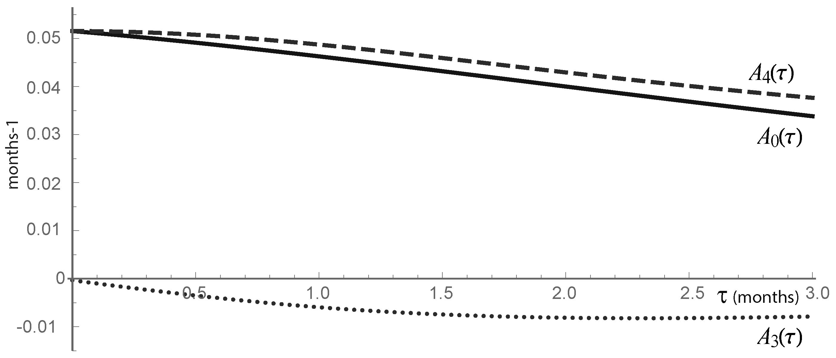
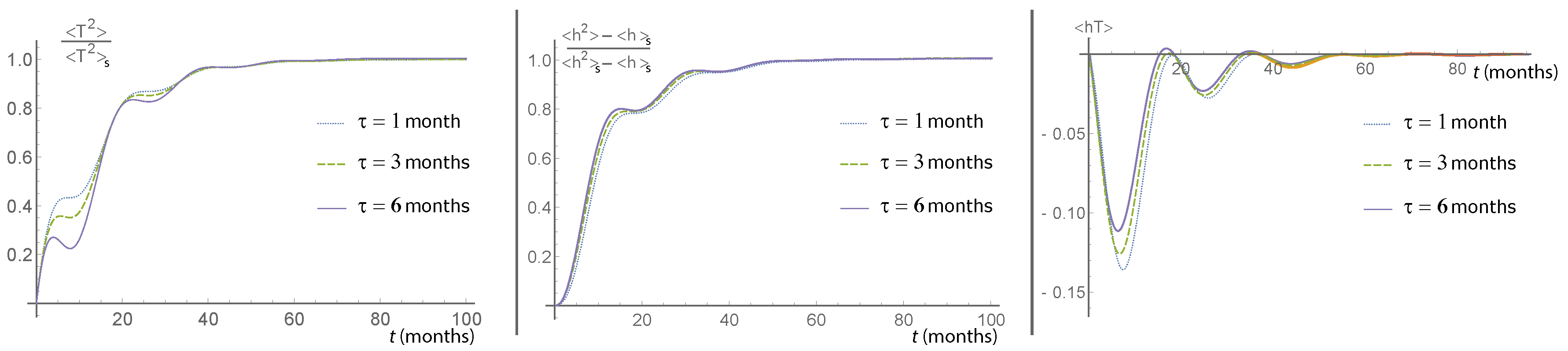
Concerning the equations of motion of the second moments (Equation (20b)), we see that they weakly depend on the B diffusion coefficient. Moreover, using the relationships of Equations (A10), (A14) and (A15), we have that they mainly depend on and ; thus, the dynamics of the second moments should not depend too much on the time scale separation between the average ROM dynamics and that of the fast forcing . Estimates of the time scale are in the range of 6–12 months. Assuming an exponential decay of the autocorrelation function of , i.e. , we can verify that for up to months, the transport coefficient A has the same structure it has in the limit of very large time scale separation (), namely (see Figure 2), and as is shown in Figure 3, the dynamics of the second moments is almost independent of .
The results of this section allow us to get two main important conclusions:
- analyzing only the first and second moments/cumulants/cross-correlation functions of the observations data, we cannot identify/detect the (possible) nonlinearity due to the interaction with the atmosphere, in the ENSO system;
- comparing the first and second moments/cumulants/cross-correlation functions, we obtain from the FPE of Equation (18) with observations, it would be really hard to determine how small the time scale of decaying of the correlation function of the effective noise perturbing the ROM is. On the other hand, as has been shown in [17], also for , the FPE of Equation (18) well accounts for the non-Gaussianity of the ENSO statistics. Thus, for the sake of simplicity, from now on, we shall use the FPE of Equation (17), which is the white noise limit of Equation (18), even if we are aware of the fact that the time scale separation between the dynamics of the averaged ROM and that of the fast atmosphere is not so “extreme”.
In the next subsection, we shall analyze Point 1 in detail.
6.2. The Covariance Matrix of the ROM and the Comparison with the ENSO Data
Given the results of the previous subsection, we assume that to describe the statistics of the ENSO, we can use the simplified FPE of Equation (17), instead of the more general Equation (18). This FPE must be validated with data from observations.
To this end, we write again the first equations for the time evolution of the first two moments, using the FPE Equation (17) (we also use the shift to ensure that the mean value of the thermocline depth anomaly is zero):
For the sake of simplicity, in the above equations, we have explicitly made the approximation of neglecting the terms proportional to , assuming that and . The validity of this assumption will be shown later. In any case, these approximations could be weakened without affecting the derivation below. From the above equations, we get the following stationary first and second moments:
The values of the ratio can be obtained from the observations with a very good accuracy. According to Equation (24), can be inferred from the variance of the Niño 3 time series, leading to (we recall that is the “standard” diffusion coefficient). For the other coefficients in the FPE of Equation (17), we focus our attention on the elements of the covariance matrix , where “x” and “y” can be either h or T. We note that by definition, we have:
where is the adjoint of the Liouvillian defined by the FPE of Equation (17). Thus, the evolutions and are solutions of the differential equations for the lowest order moments of Equation (23a). Because Equation (23a) is linear, the solutions will be linear combinations of h and T:
where:
Exploiting Equation (26), Equation (25) becomes:
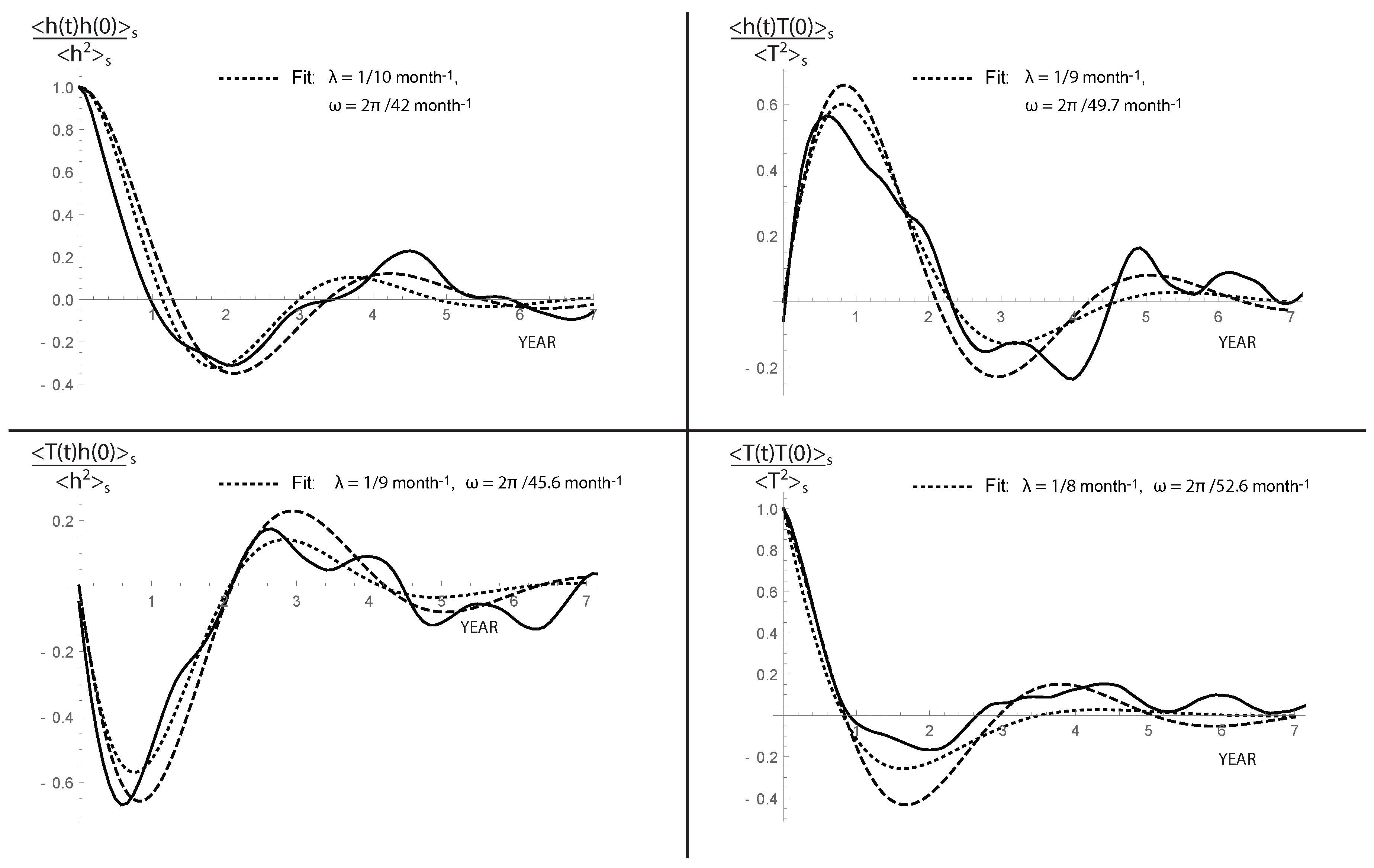
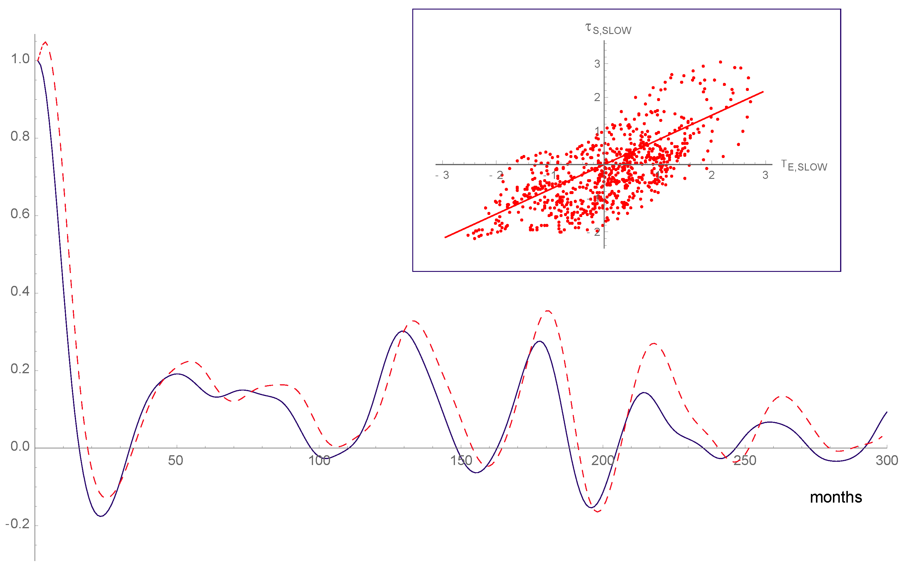
where (see Equation (24)) . In Figure 4, we show the time evolution of the elements of the correlation matrix obtained from observations and the best fit obtained with Equation (27). This best fit yields values of /48 month and month, but the residuals of these fitting functions are quite large. For that, in the same figure, we also insert the plot of the same functions of Equation (27), but with the ROM coefficients given by /48 month and month, which, as we shall see later, well agree also with other aspects of the data analysis.
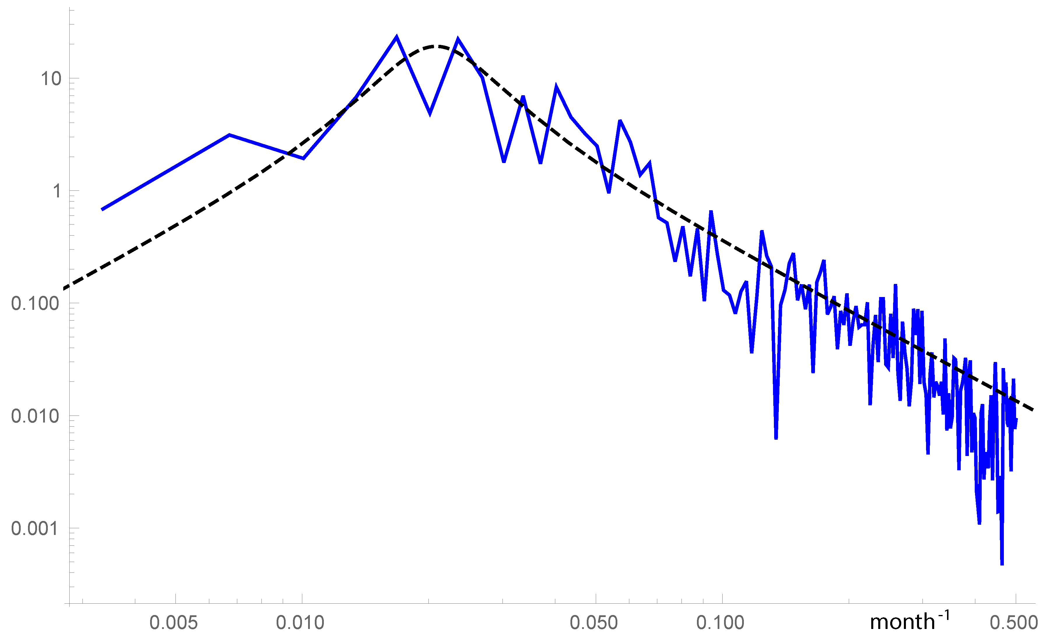
After the above results, it is not surprising that also the power spectrum analysis of the Niño 3 data shown in Figure 5 does not allow us to infer the non-Gaussian character of the ENSO statistics. In fact, although in Figure 5, the power spectrum is evaluated directly as the periodogram of the observed Niño 3 index, it is well known that it is directly related to the Fourier transform of the autocorrelation function of T, which, in our ROM with CAM forcing, does not depend on (see Equations (27) and (28)). From a quantitative point of view, the comparison of the observed and theoretical spectra in Figure 5 confirms the already found values for the unperturbed ROM parameters: /48 month, month.
6.3. Signatures of a Nonlinear Perturbation: Skewed Stationary PDF and High Frequency of Strong Events
As we have already noticed, if we focused on the first and second moments of the ENSO, we would not be able to estimate the value of the parameter responsible for the nonlinearity of the perturbed ROM of Equation (15) (or the FPE of Equation (17)). To infer the value of the parameter, we have to focus our attention on the non-Gaussian character of the ENSO statistics; hence, we have to evaluate the stationary PDF of the FPE of Equation (17). Although this FPE is simplified with respect to the more general one (Equation (18)), the exact stationary PDF is not known. It has been shown in [17], using a reasonable ansatz, that it is possible to obtain the following analytic expression for the reduced stationary PDF of the sole T variable (see also Appendix C):
where the Gamma-like density function is defined as:
in which is the standard complete Gamma function. This stationary PDF depends only on the value of the parameter that controls the relative intensity of the multiplicative part of the perturbation and on the ratio via the parameter of Equation (30). Notice that, as shown in Equation (24), is the stationary variance of T. It is easy to check analytically that in the limit and fixed, the stationary PDF in Equations (29)–(31) becomes a standard Gaussian, with the same variance . However, for , the stationary PDF is clearly non-Gaussian. In fact, for large positive T, it has a “power law” tail that makes it possible to have large fluctuations of positive values of T (strong El Niño events). From Equation (30), we have that the parameter, which controls the behavior of this “heavy” tail of the stationary PDF, strongly depends on the value of the parameter. The maximum of the stationary PDF is found at ; for fixed , it is proportional to . The probability of strong negative values of T (La Niña events) is largely reduced, and it is null for temperatures smaller than the threshold .
This skewed stationary PDF for T fits well the data from observations (see Figure 1) with and (). The value for is in agreement with the range of values we have already obtained for the variance of the ROM; hence, from now on, we set and .
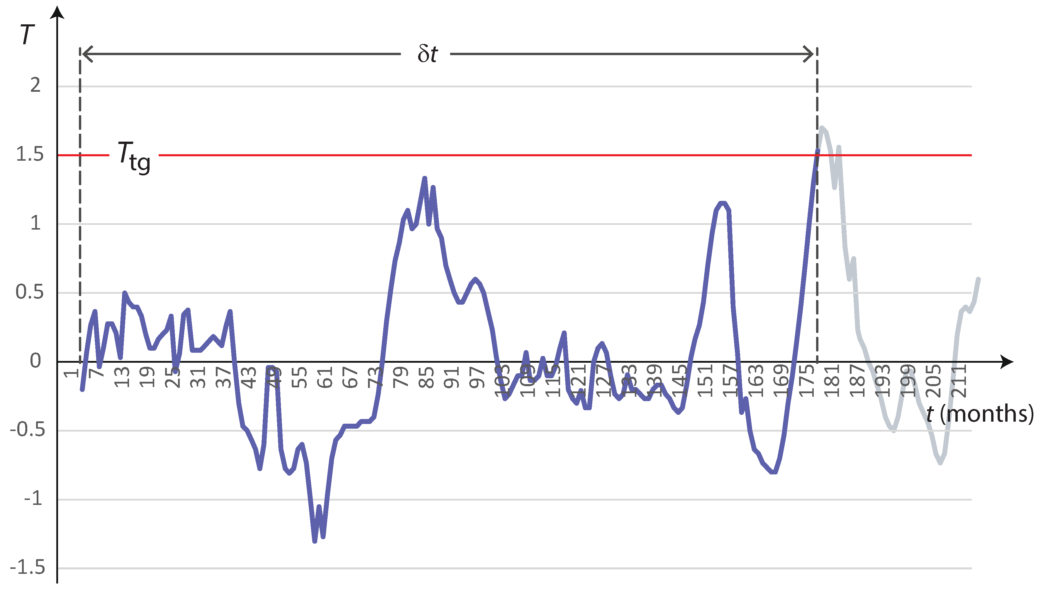
From the FPE of Equation (17) and using the same ansatz that leads to the stationary PDF in Equations (29)–(31), it is also possible to obtain an analytical expression for the mean First Passage Time (FPT) for the ENSO events [77] and to compare these results with the observations. More precisely, we are interested in the average time we have to wait for the onset of a “strong” El Niño event, starting from a “neutral” initial condition defined as the case when the temperature has a value in the range . As depicted in Figure 6, “strong” El Niño events are identified by the criterion . Thus, the FPT is defined as the time when first crosses a given target , starting from the initial value (see Figure 7). However, if is a stochastic process, repeating many times the same “experiment” should lead to different values for , so that the FPT itself is a stochastic process, with its own PDF. We indicate with the moment of the PDF of the FPT. Of course, the mean FPT is given by . As we have shown in [77], we have:
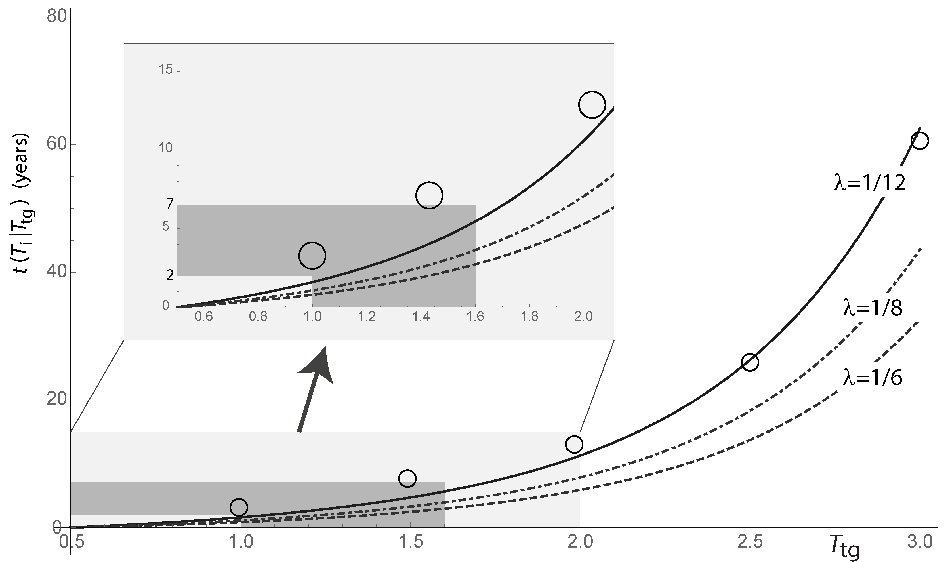
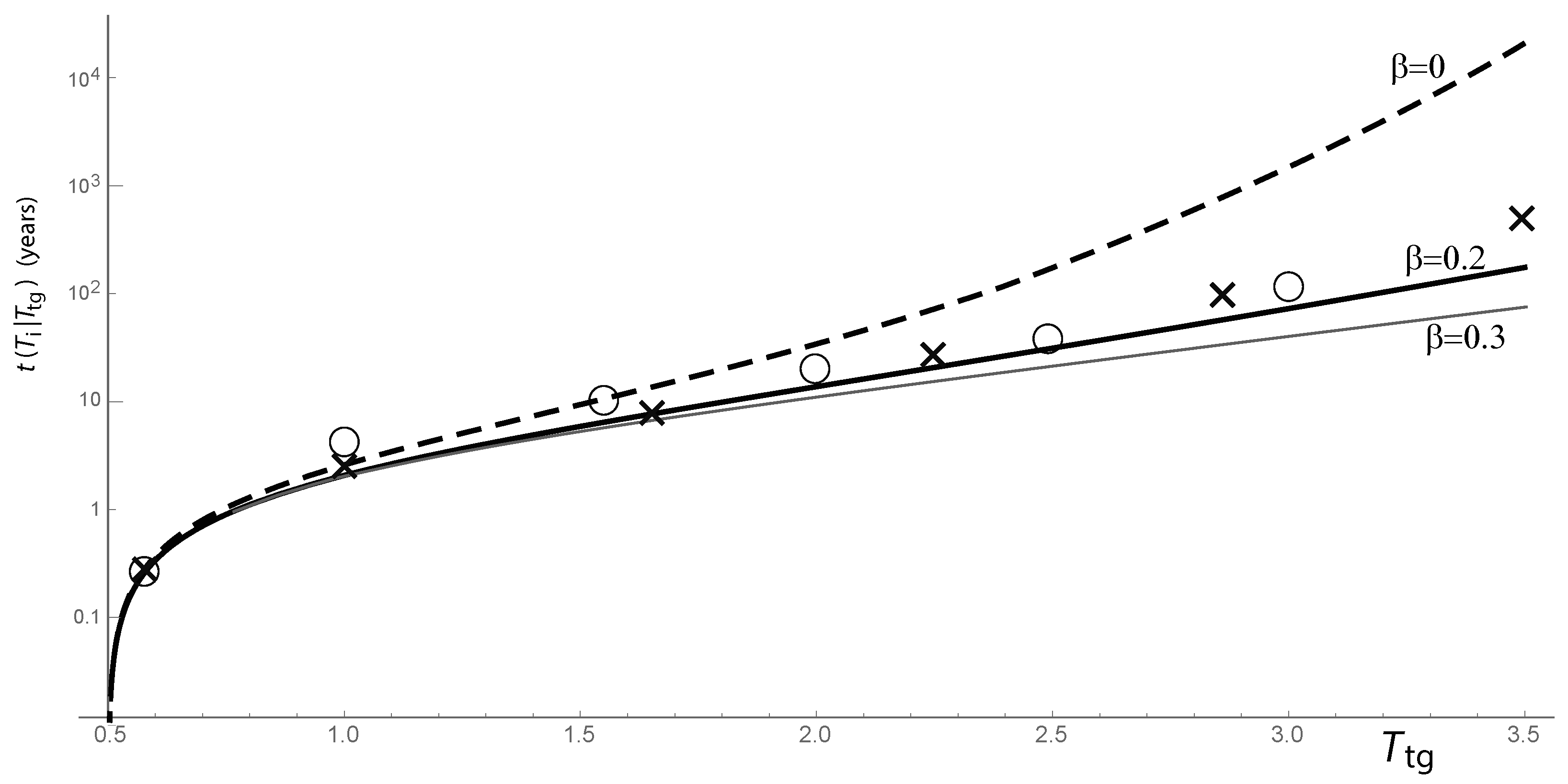
where and is the Kummers (generalized hypergeometric) function of the first kind with the first argument equal to one. We plot Equation (32) in Figure 8 to show the dependence of the mean FPT on for different values of the parameter.
From this figure, we see that months, i.e., a value at the lower end of the expected range, provides the best agreement between observational estimates and our analytic result for the mean FPT. With months, the mean FPT for intermediate target temperatures, obtained from Equation (32), is in the range of 2–7 years, in good agreement with the observed intervals between intermediate El Niño events. Apart from the inverse proportionality relationship with the relaxation coefficient , it is also clear that the average FPT has a strong sensitivity to the value of the parameter (once the variance is kept fixed, the parameter depends only on as ). In Figure 9, we compare the average FPT of Equation (32) with the values obtained through the numerical integration of the stochastic differential equation equivalent to the FPE of Equation (17) using . We can see that there is a good agreement between the analytical and numerical solutions. In the same figure, we also show the analytical solutions of the average FPT in the case of a pure additive perturbation (, in which case, the reduced stationary PDF for the T variable is Gaussian) and for . For weak to intermediate El Niño events (), the average FPT depends weakly on . However, the sensitivity to clearly emerges in the case of strong and very strong events. In particular, the purely additive forcing leads to average FPT that are many orders of magnitude larger than those obtained with (note the logarithmic scale in the ordinate of the graph), while in the case of , the FPTs are shorter at large .
Notice that strong and very strong ENSO are extreme events, and as such, they are rare, so that it is not possible to have a sufficiently large observational sample size to validate in detail the analytical results. In fact, we do not use these extreme events to estimate the value of ( has been estimated by fitting to data the theoretical PDF of Equation (29), and it is compatible with both the observed negative value for the maximum of the PDF and its kurtosis). The other way around, we can use our analytical solution with as a reasonable extrapolation of the mean FPT for these strong or very strong El Niños, and the fact that this extrapolation fits well to the (few) available data is encouraging.
6.4. Inferring the FPE Coefficients from Data
The results of the previous sections validate the FPE of Equation (17) with parameters /48 month, month and . However, at least in principle, there is a way to infer the transport coefficients of an FPE directly from data. For that purpose, let us rewrite the FPE of Equation (17) in the following way:
where (as in Equation (23) we used the transformation to eliminate the mean value of the thermocline depth anomaly):
It is well known that given the FPE of Equation (17), the drift and diffusion coefficients can be inferred using their statistical definitions as conditional first and second moments of the process increments [80,81,82]:
in which is the conditional probability to go from to in an infinitesimal time . From a practical viewpoint, the above expressions are obtained from the expectation values of the first (Equations (35b) and (35c)) and second (Equation (35a)) moments of the difference of two subsequent Niño 3 values, where the time step is month. Because the duration of the h time series is too short to obtain a reliable two-dimensional PDF (note that for h, we use the “proxy” given by the anomalies in the volume of Warm Water (WWV) in the basin 120 E–80 W, 5 S–5 N, in the time range from January 1982–December 2017, taken from [76]), we focus our attention only on the T variable, i.e., we work only with the observed Niño 3 index. This means that we disregard the drift coefficient of Equation (35c), and for each T value, when we evaluate the expectation of the first and second moments of the process increments of T, we automatically average over h at fixed T. This average over the h variable does not affect the diffusion coefficient of Equation (35a), thus,
while for the drift coefficient of Equation (35b), we have:
where means the conditional stationary average at fixed T, and in the second line, we have exploited the ansatz introduced in [17] (see also Appendix C).
The functions in Equations (36) and (37)) correspond to the diffusion and drift coefficients, respectively, of the following reduced FPE for the T variable:
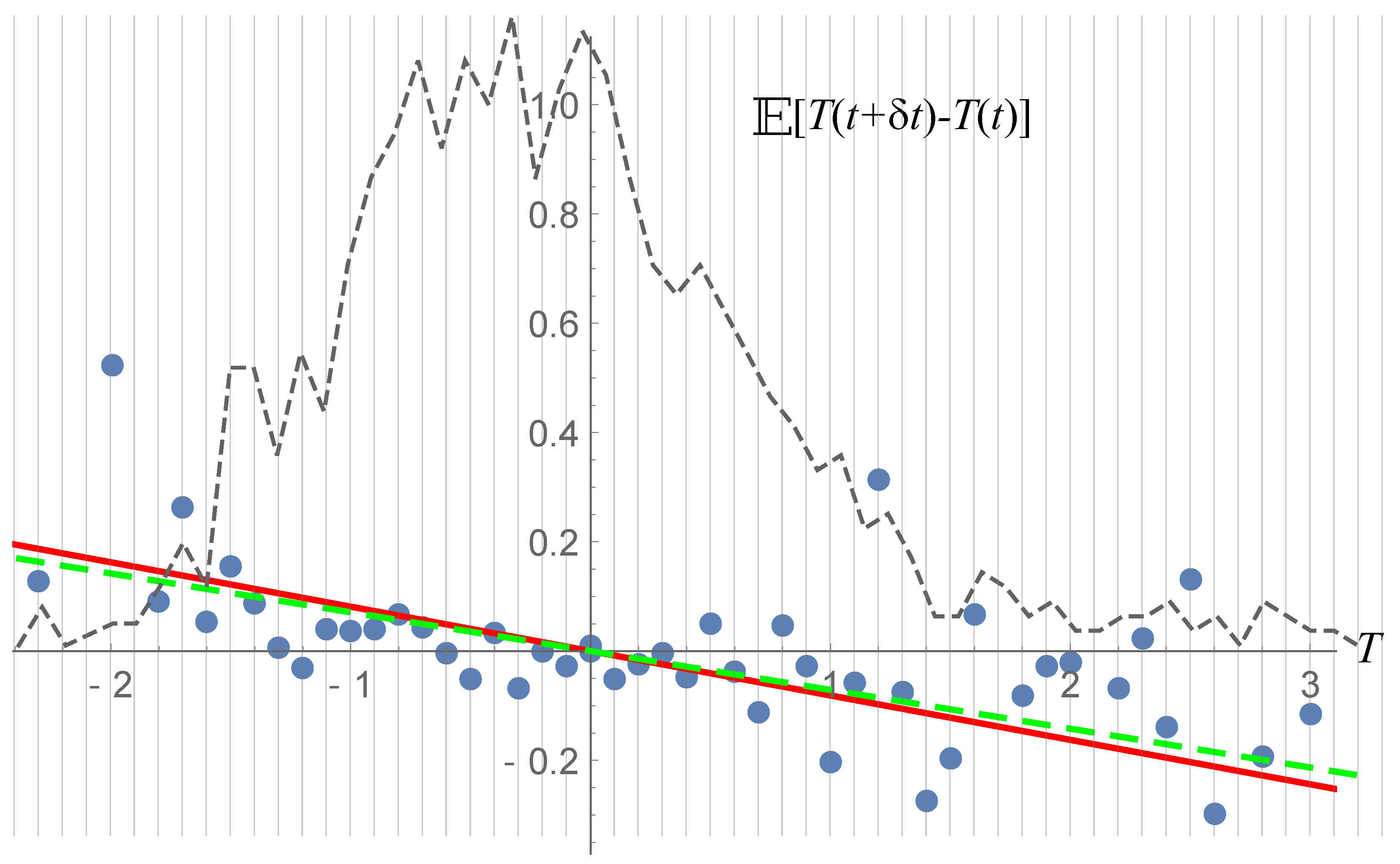
that is, the same FPE we would obtain directly by using the already cited ansatz introduced in [17], in the FPE of Equations (17)–(34). In Figure 10, we see that from the Niño 3 data, the expectation value, looks as a linear function of T, supporting again the view of a linear unperturbed ROM, and the linear fit is very close to with month, the same values we have obtained from the mean FPT analysis of the previous subsection.
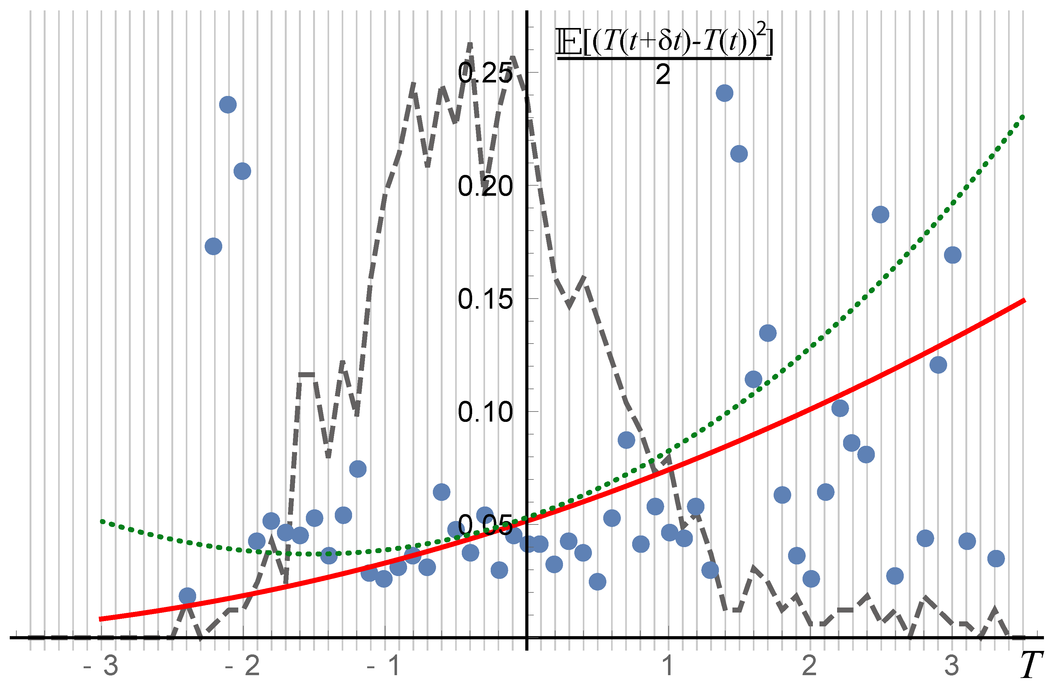
Concerning the diffusion coefficient, evaluated as in Equation (35a), we see from Figure 11 that the expectation value is compatible with the square dependence on T of Equation (36), but the the uncertainty is large. This large uncertainty is due to the nonlinear nature of , which makes the fitting process strongly dependent on large T values where the statistics is poor. The large value of the for large negative T () suggests that could be quite larger than (leading to a diffusion term more symmetric with respect to zero compared with the case ); however, in this case, it would be necessary to add another noise term, additive and uncorrelated with the CAM one, to explain the other results so far presented. Actually, this is the perturbation already introduced in Equation (16), and the corresponding diffusion coefficient is shown in the same Figure 11 as a dashed green line. The case where an additional uncorrelated noise is added to the present perturbed ROM will be deeply analyzed in a forthcoming work.
7. Discussion and Conclusions
Starting from the fact that the ENSO statistics has some clear non- Gaussian features, in this paper, we use the results of some recent papers, and we analyze further the statistics of the ENSO, with the specific goal of discussing which non-linear dynamics might be responsible for them. Thus, as in [17], we work with the Fokker–Planck Equation (FPE) for the PDFof the ROM variables, but here aiming at the search for nonlinearities. In this simplified model, we consider two possible sources of nonlinearities: nonlinearity in the dynamics of the unperturbed ROM and a nonlinear (i.e., multiplicative) fast perturbation of the ROM.
Comparison with observations leads to the conclusion that a possibly nonlinear interaction between the internal ROM variables cannot be inherently the cause of the observed non-Gaussianity, which instead is well reproduced assuming a linear ROM with a nonlinear chaotic perturbation.
The hypothesis of nonlinear interaction between the unperturbed ROM and the fast forcing is strongly supported by the comparison between observations and theoretical results (stationary PDF and average FPT) for values of T where the number of observation data is statistically relevant (weak and intermediate ENSO).
It is noticeable that extrapolating this result also for large T, the heavy tail of the PDF leads to relatively short recurring times of strong ENSO, which still fit well to the few observations and that are orders of magnitude smaller than those we would have in the Gaussian case.
In Section 6.4 for the first time, observation data are used to infer directly the FPE coefficients. In this way, we are able to validate once more the assumption of a linear internal dynamics of the ROM (Figure 10) and of a non-constant diffusion (Figure 11) coefficient. At a quantitative level, however, the exact relationship between T and the diffusion coefficient is difficult to determine in this way because nonlinearities become important in the large T range (rare events), where the statistics is rather poor (dashed line in Figure 11).
We can conclude that the nonlinear interaction between the fast and slow modes of the ENSO gives a substantial contribution to the non-Gaussianity of the ENSO statistics. However, further work is necessary to better quantify the nonlinear nature of the perturbation, which is related to the nonlinear diffusion coefficient of the FPE. For example, from observations, we see that the expectation value , which should reproduce the functional dependence of the diffusion coefficient with respect to the T variable, is compatible with the CAM diffusion term of Equation (36) with a small beta (), but also with the case where there is another diffusion coefficient , in this case constant. In fact, it turns out that the sum fits to the data, as well as alone (see in Figure 11), but with an increased value for and a decreased value for D (the sum must be kept fixed to preserve the value of the variance). Thus, to be able to define the actual and values, we should increase the sample size used for the fitting process, for example using longer time series from century-long reanalysis products (CERA 20C, https://www.ecmwf.int/en/forecasts/datasets/archive-datasets/reanalysis-datasets/cera-20c) and/or proxy data (networks of precipitation, tree-rings, corals and ice core records) that can help extend the time series back in time some hundreds of years [83]. Another point that deserves more investigation is the role of the weak nonlinearity in the interaction between the ROM variables h and T, under the current assumption of the nonlinear perturbation. In fact, in Section 3, we have assumed a linear (i.e., additive) perturbation to show that the internal nonlinearities cannot be the cause of the observed non-Gaussianity of the Niño 3 PDF. However, how much does the internal nonlinearity affect the PDF in the case of a nonlinear interaction? This is not a trivial question because, as we have shown in this paper, the nonlinear interaction leads to a much slower decay of the PDF, with respect to the linear (i.e., additive) case, and the tails of the PDF are where the small nonlinear terms can emerge. These are all issues on which we are currently working.
Author Contributions
Conceptualization, M.B. Formal analysis, M.B., R.M. and S.M. Data, M.B., R.M., S.M. and A.C. Methodology, M.B., R.M. and A.C. Validation, R.M. and A.C. Writing—original draft, M.B. and S.M. Writing—review and editing, M.B., A.C., R.M. and S.M.
Funding
This research received no external funding.
Conflicts of Interest
The authors declare no conflict of interest.
Appendix A. Validation of the Linear Relationship between the Wind Stress and TE
Equation (4) is an assumption that agrees with observations, as shown in the following. The wind stress is considered proportional to the square of the wind velocity at 10 m from the sea surface, taken from [61]. Figure A1 shows the equatorial zonal (i.e., averaged over 5 S–5 N) wind velocity for different longitudes. We see that very close to the Americas’ coasts (81 W), the direction of the wind flips from trade wind to westerly. This is due to the thermal gradient we have when we pass from the cold East Pacific Equatorial Ocean to the warm Central American lands. Thus, for the wind stress of Equation (4), we use the anomaly (i.e., 1948–2018 mean removed) of the equatorial zonal wind stress averaged in the longitude interval 180 W–120 W. The fluctuating quantity is divided into slow () and fast () components. The data are obtained from the one-year average of data, while . Then:
- (1)
- From Figure A2, we clearly see that the time behaviors of and are similar (of course, some lag remains between the wind stress, which is a a forcing term, and the ocean reaction);
- (2)
- From Figure A3, we see that the plot of the cross-correlation between and vs. time (in moths) is very similar to the plot of the autocorrelation of (notice the little time offset between these two plots, indicating the fact that the one-year time average has not completely hidden the cause-effect relationship between and ). Moreover, from the insert of the same figure, we see that the average relationship between and is mainly linear, with a small dispersion of the data around the linear fit (quantities are normalized by the standard deviation of the quantities from observations):
The above two arguments strongly support the hypothesis expressed by Equation (4).
Figure A1.
5N–5S averaged zonal wind for different longitudes. Data from NOAA [61].
Figure A1.
5N–5S averaged zonal wind for different longitudes. Data from NOAA [61].

Appendix B. Very Short Review of the Projection Approach Applied to the ROM
In the present work, we study the same ROM considered in [17]; however, we do not use the FPE in Equations (3) and (4) of [17] because of a marginal mistake: a missing additive term in the FPE, which here we want to fix. Thus, for the reader’s convenience, in the following, we give a short summary of the projection procedure adapted to the present case.
The idea of this approach is to assume that the fast fluctuating force has a deterministic nature, namely that the ROM of Equation (15) is just a part of a set of equations describing a larger deterministic system:
Using the terminology of the projection approach [27,66,84], the ROM is viewed as the “system of interest” (or system a), while represents the booster system (or “rest of the system” or system b), namely a set of general chaotic and fast variables, e.g., the MJO and WWB [85,86,87,88,89], which, perturbing the ROM, activate the El Niño/La Niña phenomena and which obey some unspecified equations of motion expressed by the generic functions and . The value of the parameter determines the intensity of the perturbation to the ROM. For , the first two lines of Equation (A2) define the unperturbed system of interest (or unperturbed ROM).
We stress that we leave unspecified the exact expressions of the functions and , representing the equation of motion for the booster, because we do not need to know them in detail (the booster typically will be a nonlinear chaotic system); it is enough that they satisfy some specific assumptions, as detailed in the following.
More generally, the interaction between the ROM and the booster should be bi-directional: the booster equation of motion should be affected by the dynamics of the ROM: and . The function is the “reaction” force of the ROM variables on the MJO/WWB system. However, for the sake of simplicity, we shall consider hereafter as in [17]. The feedback term can be included following the general approach of [26,33]. The goal is to describe the statistics of the part of interest. We start from the following Langevin equation for the PDF of the total system:
where the unperturbed and perturbation Liouville operators are given by:
respectively. In Equation (A3), we do not write the explicit expression of the Liouville operator of the booster because it is related to the unknown functions and .
We are interested in obtaining a Fokker–Plank Equation (FPE) for the reduced (or marginal) PDF of the system of interest, given by . Introducing the projection operator, , where is the stationary PDF of the booster, defined by , we have: . Following the Zwanzig-like formal projection approach in the perturbation version of [64,65,66] to the lowest non-vanishing order on the coupling parameter , the time evolution of is governed by the following integro-differential equation:
In the above equation, is the normalized auto-correlation function of the booster variable and is the variance of (without any loss of generality, we assumed ). A very important outcome of Equation (A5) is that we can group all the possible booster dynamical systems in different classes of equivalence, where all the boosters belonging to the same class give rise to the same statistical properties for a given system of interest. In fact, the FPE depends only on the booster autocorrelation function : different dynamical systems that share the same autocorrelation function belong to the same booster class of equivalence. Given Equation (A4), we can rewrite Equation (A5) as:
where we have used the identity (this last term was the cited missed one in [17], and it is not vanishing when the interaction with the booster is not Hamiltonian, as in the present case), and we have introduced the decay time of the booster autocorrelation function as . Moreover, in the above equation, we have exploited the result (see for example Equations (31) and (32) of [27]), where and (for further use) are the unperturbed () back time evolution for a time u of the T and the h variables, respectively, starting from the initial condition () given by and .
In the case where there is an extremely large time scale separation between the dynamics of the unperturbed ROM and the forcing atmosphere, the autocorrelation function decays so fast, with respect to the typical time scale of the unperturbed ROM, that we can make the following approximations: and . Thus, in this case, from Equation (A6), we obtain the standard result of the theory of stochastic Markovian processes [74], namely the FPE of Equation (17).
More in general, Equation (A6) gives the transport coefficients and of Equation (18), also for the cases where we do not assume such stringent assumptions about the time scale separation between the unperturbed ROM and the fast atmosphere. These have been already given in the Supporting Information of [17], by making a link with some final results of [27]. We mention only the fact that the most troublesome problem in order to get and from Equation (A6) is to manipulate the compound of operators . For that, we refer the reader to the results of [33] and (for a more general approach to the Lie evolution of differential operators) to the more recent work of [32]. Here, we report the final result, which is given by Equation (19), where ():
with , and the symbols and stand for the imaginary and the real part of , respectively, and the hat over the function means the Fourier transform of this function, having assumed for : . The following equalities hold:
Appendix C. The Ansatz and the Stationary PDF
Here, we review Appendix B of [17], to find the reduced stationary PDF for the T variable. We start from the FPE of Equation (17), which, after the shift , which annuls the mean value of the anomaly thermocline depth, becomes the FPE of Equations (33) and (34). Because we are interested only in the reduced PDF for the T variable, we integrate the h variable in the FPE of Equations (33) and (34), to obtain (we remind again that ):
where is the reduced PDF for the T variable and is the conditional average value of the h variable (note: ). Because and , we are neither in the under-damped, nor in the over-damped standard cases where it is possible to reduce the two-dimensional FPE to the one-dimensional type [42,65,90]. However, we take advantage of the fact that here, we focus our attention on the stationary PDF of the reduced FPE, for which in Equation (A16). Thus, observing that the relations among the stationary first and second moments of the h and T variables that we obtain from Equation (23) are the same for the case of a stochastic damped linear oscillator (see also B_16), we make the following ansatz:
where the former equality represents the ansatz.
Inserting Equation (A17) in the FPE of Equation (A16), imposing the condition of vanishing current and using the definition , we obtain:
From the previous equation, we get two results: the stationary PDF has a maximum (i.e., the T derivative vanishes) for ; the stationary PDF must vanish for (and for lesser values as well, for obvious physical reasons). As already noted in [17], from Equation (23), for (namely, for ), the equation of motion of the first and second order moments of the ROM converge to a finite value for . It is not difficult to check that the same constraint ensures that also the solution of the FPE of Equation (17) converges, for , to a finite (normalizable) stationary PDF. Thus, under the assumption that , from Equation (A18), we get the stationary PDF given in Equation (29).
Figure A2.
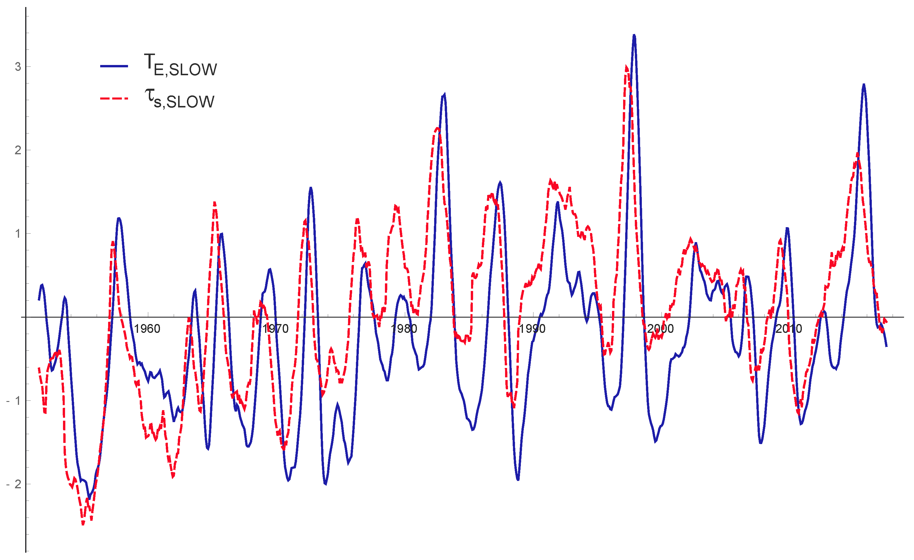
Plot of the 13-month averaged Niño 3 data (blues solid line) and of the 13-month averaged wind stress anomaly (dashed red line). Quantities are normalized by their respective standard deviations. The Niño 3 data are from [50], while the wind stress is proportional to the square of the wind velocity, where the wind data are from [61]. The wind stress has been averaged on the equatorial strip defined by (5 S–5 N) × (120 W–180 W).
Figure A2.
Plot of the 13-month averaged Niño 3 data (blues solid line) and of the 13-month averaged wind stress anomaly (dashed red line). Quantities are normalized by their respective standard deviations. The Niño 3 data are from [50], while the wind stress is proportional to the square of the wind velocity, where the wind data are from [61]. The wind stress has been averaged on the equatorial strip defined by (5 S–5 N) × (120 W–180 W).

Figure A3.
Blue solid line: normalized auto-correlation of the one-year averaged Niño 3 index: . Red-dashed line: cross-correlation between the and , normalized with the initial value: . We can see that they are very similar to each other. Insert: vs. (red dots). Data from NOAA [50] (Niño 3) and [61] (wind).

References
- Larkin, N.K.; Harrison, D.E. ENSO Warm (El Niño) and Cold (La Niña) Event Life Cycles: Ocean Surface Anomaly Patterns, Their Symmetries, Asymmetries, and Implications. J. Clim. 2002, 15, 1118–1140. [Google Scholar] [CrossRef]
- Kug, J.S.; Ham, Y.G. Are there two types of La Nina? Geophys. Res. Lett. 2011, 38. [Google Scholar] [CrossRef] [Green Version]
- An, S.I. Interdecadal changes in the El Nino-La Nina asymmetry. Geophys. Res. Lett. 2004, 31. [Google Scholar] [CrossRef] [Green Version]
- An, S.I.; Kim, J.W. Role of nonlinear ocean dynamic response to wind on the asymmetrical transition of El Niño and La Niña. Geophys. Res. Lett. 2017, 44, 393–400. [Google Scholar] [CrossRef]
- Dommenget, D.; Bayr, T.; Frauen, C. Analysis of the non-linearity in the pattern and time evolution of El Niño southern oscillation. Clim. Dyn. 2013, 40, 2825–2847. [Google Scholar] [CrossRef]
- Frauen, C.; Dommenget, D. El Niño and La Niña amplitude asymmetry caused by atmospheric feedbacks. Geophys. Res. Lett. 2010, 37, L18801. [Google Scholar] [CrossRef]
- Moore, A.M.; Kleeman, R. The dynamics of error growth and predictability in a coupled model of ENSO. Q. J. R. Meteorol. Soc. 1996, 122, 1405–1446. [Google Scholar] [CrossRef]
- Penland, C.; Sardeshmukh, P.D. The Optimal Growth of Tropical Sea Surface Temperature Anomalies. J. Clim. 1995, 8, 1999–2024. [Google Scholar] [CrossRef] [Green Version]
- Weiss, J.B. Fluctuation properties of steady-state Langevin systems. Phys. Rev. E 2007, 76, 061128. [Google Scholar] [CrossRef] [PubMed]
- Jin, F.F. An Equatorial Ocean Recharge Paradigm for ENSO. Part II: A Stripped-Down Coupled Model. J. Atmos. Sci. 1997, 54, 830–847. [Google Scholar] [CrossRef]
- Jin, F.F. An Equatorial Ocean Recharge Paradigm for ENSO. Part I: Conceptual Model. J. Atmos. Sci. 1997, 54, 811–829. [Google Scholar] [CrossRef]
- Burgers, G.; Jin, F.F.; van Oldenborgh, G.J. The simplest ENSO recharge oscillator. Geophys. Res. Lett. 2005, 32, L13706. [Google Scholar] [CrossRef]
- Capotondi, A.; Wittenberg, A.; Masina, S. Spatial and temporal structure of Tropical Pacific interannual variability in 20th century coupled simulations. Ocean Model. 2006, 15, 274–298. [Google Scholar] [CrossRef]
- Jin, F.F.; Lin, L.; Timmermann, A.; Zhao, J. Ensemble-mean dynamics of the ENSO recharge oscillator under state-dependent stochastic forcing. Geophys. Res. Lett. 2007, 34, L03807. [Google Scholar] [CrossRef]
- Levine, A.F.Z.; Jin, F.F. Noise-Induced Instability in the ENSO Recharge Oscillator. J. Atmos. Sci. 2010, 67, 529–542. [Google Scholar] [CrossRef] [Green Version]
- Ren, H.L.; Jin, F.F. Recharge Oscillator Mechanisms in Two Types of ENSO. J. Clim. 2013, 26, 6506–6523. [Google Scholar] [CrossRef]
- Bianucci, M. Analytical probability density function for the statistics of the ENSO phenomenon: Asymmetry and power law tail. Geophys. Res. Lett. 2016, 43, 386–394. [Google Scholar] [CrossRef]
- Battisti, D.S.; Hirst, A.C. Interannual variability in a tropical atmosphere-ocean model: Influence of the basic state, ocean geometry and nonlinearity. J. Atmos. Sci. 1989, 46, 1687–1712. [Google Scholar] [CrossRef]
- Mantua, N.J.; Battisti, D.S. Evidence for the Delayed Oscillator Mechanism for ENSO: The “Observed” Oceanic Kelvin Mode in the Far Western Pacific. J. Phys. Oceanogr. 1994, 24, 691–699. [Google Scholar] [CrossRef] [Green Version]
- Im, S.H.; An, S.I.; Kim, S.T.; Jin, F.F. Feedback processes responsible for El Niño-La Niña amplitude asymmetry. Geophys. Res. Lett. 2015, 42, 5556–5563. [Google Scholar] [CrossRef] [Green Version]
- Sardeshmukh, P.D.; Penland, C. Understanding the distinctively skewed and heavy tailed character of atmospheric and oceanic probability distributions. Chaos 2015, 25, 036410. [Google Scholar] [CrossRef] [PubMed] [Green Version]
- Sardeshmukh, P.D.; Sura, P. Reconciling Non-Gaussian Climate Statistics with Linear Dynamics. J. Clim. 2009, 22, 1193–1207. [Google Scholar] [CrossRef] [Green Version]
- Sura, P.; Sardeshmukh, P.D. A global view of air-sea thermal coupling and related non-Gaussian {SST} variability. Atmos. Res. 2009, 94, 140–149. [Google Scholar] [CrossRef]
- Sardeshmukh, P.D.; Compo, G.P.; Penland, C. Need for Caution in Interpreting Extreme Weather Statistics. J. Clim. 2015, 28, 9166–9187. [Google Scholar] [CrossRef]
- Penland, C.; Sardeshmukh, P.D. Alternative interpretations of power-law distributions found in nature. Chaos Interdiscip. J. Nonlinear Sci. 2012, 22, 023119. [Google Scholar] [CrossRef] [PubMed]
- Bianucci, M.; Merlino, S. Non Standard Fluctuation Dissipation Processes in Ocean-Atmosphere Interaction and for General Hamiltonian or Non Hamiltonian Phenomena: Analytical Results; Mathematics Research Developments, Nova Science Publisher: Hauppauge, NY, USA, 2017. [Google Scholar]
- Bianucci, M. On the correspondence between a large class of dynamical systems and stochastic processes described by the generalized Fokker Planck equation with state-dependent diffusion and drift coefficients. J. Stat. Mech. Theory Exp. 2015, 2015, P05016. [Google Scholar] [CrossRef]
- Dorfman, J.R. An Introduction to Chaos in Nonequilibrium Statistical Mechanics; Cambridge Lecture Notes in Physics; Cambridge University Press: Cambridge, UK, 1999. [Google Scholar]
- Zwanzig, R. (Ed.) Nonequilibrium Statistical Mechanics; Oxford University Press: Oxford, UK, 2001. [Google Scholar]
- Chorin, A.J.; Hald, O.H.; Kupferman, R. Optimal prediction and the Mori-Zwanzig representation of irreversible processes. Proc. Natl. Acad. Sci. USA 2000, 97, 2968–2973. [Google Scholar] [CrossRef] [PubMed] [Green Version]
- Grigolini, P.; Marchesoni, F. Basic Description of the Rules Leading to the Adiabatic Elimination of Fast Variables. In Advances in Chemical Physics: Memory Function Approaches to Stochastich Problems in Condensed Matter; Evans, M.W., Grigolini, P., Parravicini, G.P., Eds.; John Wiley & Sons: New York, NY, USA, 1985; Volume 62, p. 556. [Google Scholar]
- Bianucci, M. Using some results about the Lie evolution of differential operators to obtain the Fokker-Planck equation for non-Hamiltonian dynamical systems of interest. J. Math. Phys. 2018, 59, 053303. [Google Scholar] [CrossRef]
- Bianucci, M. Large Scale Emerging Properties from Non Hamiltonian Complex Systems. Entropy 2017, 19, 302. [Google Scholar] [CrossRef]
- Smoluchowski, M.V. Irregularity in the distribution of gaseous molecules and its influence. Boltzmann Festschr. 1904, 626–641. [Google Scholar]
- Smoluchowski, M.V. Theory of the Brownian movements. Bull. Acad. Sci. Crac. 1906, 577–602. [Google Scholar]
- Schadschneider, A.; Chowdhury, D.; Nishinari, K. (Eds.) Stochastic Transport in Complex Systems. From Molecules to Vehicles; Elsevier: Amsterdam, The Netherlands, 2010. [Google Scholar]
- Kampen, N.V. (Ed.) Stochastic Processes in Physics and Chemistry, 3rd ed.; Elsevier: Amsterdam, The Netherlands, 2007. [Google Scholar]
- Risken, H. The Fokker-Planck Equation. Methods of Solution and Applications; Springer: Berlin/Heidelberg, Germany, 1996; Volume 18. [Google Scholar]
- Kubo, R.; Toda, M.; Hashitsume, N. Statistical Physics II. Nonequilibrium Statistical Mechanics; Springer: Berlin/Heidelberg, Germany, 1985; Volume 31. [Google Scholar]
- Ding, M.; Rangarajan, G. First Passage Time Problem: A Fokker-Planck Approach. In New Directions in Statistical Physics: Econophysics, Bioinformatics, and Pattern Recognition; Wille, L.T., Ed.; Springer: Berlin/Heidelberg, Germany, 2004; pp. 31–46. [Google Scholar]
- Kramers, H. Brownian motion in a field of force and the diffusion model of chemical reactions. Physica 1940, 7, 284–304. [Google Scholar] [CrossRef]
- Bianucci, M.; Grigolini, P.; Palleschi, V. Beyond the linear approximations of the conventional approaches to the theory of chemical relaxation. J. Chem. Phys. 1990, 92, 3427–3441. [Google Scholar] [CrossRef]
- Bianucci, M. Ordinary chemical reaction process induced by a unidimensional map. Phys. Rev. E 2004, 70, 026107. [Google Scholar] [CrossRef] [PubMed]
- Revelli, J.A.; Budde, C.E.; Wio, H.S. Diffusion in fluctuating media: First passage time problem. Phys. Lett. A 2002, 306, 104–109. [Google Scholar] [CrossRef]
- Kulkarni, V.G.; Tzenova, E. Mean first passage times in fluid queues. Oper. Res. Lett. 2002, 30, 308–318. [Google Scholar] [CrossRef]
- Giorno, V.; Nobile, A.; Ricciardi, L. Single neuron’s activity: On certain problems of modeling and interpretation. Biosystems 1997, 40, 65–74. [Google Scholar] [CrossRef]
- Tuckwell, H.C. (Ed.) Introduction to Theoretical Neurobiology; Cambridge Studies in Mathematical Biology; Cambridge University Press: Cambridge, UK, 2006. [Google Scholar]
- Kurzyński, M.; Chełminiak, P. Mean First-Passage Time in the Stochastic Theory of Biochemical Processes. Application to Actomyosin Molecular Motor. J. Stat. Phys. 2003, 110, 137–181. [Google Scholar] [CrossRef]
- Brics, M.; Kaupuzs, J.; Mahnke, R. How to solve Fokker-Planck equation treating mixed eigenvalue spectrum? Condens. Matter Phys. 2013, 16, 1–13. [Google Scholar] [CrossRef]
- NOAA Climate Prediction Center. Available online: https://www.cpc.ncep.noaa.gov/data/indices/ (accessed on 20 June 2018).
- Philander, S.G.H. The Response of Equatorial Oceans to a Relaxation of the Trade Winds. J. Phys. Oceanogr. 1981, 11, 176–189. [Google Scholar] [CrossRef] [Green Version]
- Jin, F.F.; Neelin, J.D. Modes of Interannual Tropical Ocean-Atmosphere Interaction—A Unified View. Part I: Numerical Results. J. Atmos. Sci. 1993, 50, 3477–3503. [Google Scholar] [CrossRef]
- Neelin, J.D.; Jin, F.F. Modes of Interannual Tropical Ocean-Atmosphere Interaction—A Unified View. Part II: Analytical Results in the Weak-Coupling Limit. J. Atmos. Sci. 1993, 50, 3504–3522. [Google Scholar] [CrossRef]
- Khas’minskii, R. A Limit Theorem for the Solutions of Differential Equations with Random Right-Hand Sides. Theory Probab. Appl. 1966, 11, 390–406. [Google Scholar] [CrossRef]
- Gallavotti, G.; Cohen, E.G.D. Dynamical ensembles in stationary states. J. Stat. Phys. 1995, 80, 931–970. [Google Scholar] [CrossRef] [Green Version]
- Gallavotti, G.; Cohen, E.G.D. Dynamical Ensembles in Nonequilibrium Statistical Mechanics. Phys. Rev. Lett. 1995, 74, 2694–2697. [Google Scholar] [CrossRef] [PubMed]
- Terwiel, R. Projection operator method applied to stochastic linear differential equations. Physica 1974, 74, 248–265. [Google Scholar] [CrossRef]
- Da-jin, W.; Li, C.; Bo, Y. Probability Evolution and Mean First-Passage Time for Multidimensional Non-Markovian Processes. Commun. Theor. Phys. 1989, 11, 379. [Google Scholar] [CrossRef]
- Kampen, N.V. Elimination of fast variables. Phys. Rep. 1985, 124, 69–160. [Google Scholar] [CrossRef]
- Kim, S.T.; Jin, F.F. An ENSO stability analysis. Part II: Results from the twentieth and twenty-first century simulations of the CMIP3 models. Clim. Dyn. 2011, 36, 1609–1627. [Google Scholar] [CrossRef]
- NOAA ESRL, NCEP/NCAR Reanalysis Data. Available online: https://www.esrl.noaa.gov/psd/data/gridded/data.ncep.reanalysis.derived.surfaceflux.html (accessed on 20 June 2018).
- Wen, C.; Kumar, A.; Xue, Y.; McPhaden, M.J. Changes in Tropical Pacific Thermocline Depth and Their Relationship to ENSO after 1999. J. Clim. 2014, 27, 7230–7249. [Google Scholar] [CrossRef]
- Bianucci, M. Nonconventional fluctuation dissipation process in non-Hamiltonian dynamical systems. Int. J. Mod. Phys. B 2015, 30, 1541004. [Google Scholar] [CrossRef]
- Grigolini, P. The projection approach to the Fokker-Planck equation: Applications to phenomenological stochastic equations with coloured noises. In Noise in Nonlinear Dynamical Systems; Moss, F., McClintock, P.V.E., Eds.; Cambridge University Press: Cambridge, UK, 1989; Volume 1, Chapter 5; p. 161. [Google Scholar]
- Bianucci, M.; Grigolini, P. Nonlinear and non Markovian fluctuation-dissipation processes: A Fokker-Planck treatment. J. Chem. Phys. 1992, 96, 6138–6148. [Google Scholar] [CrossRef]
- Bianucci, M.; Mannella, R.; West, B.J.; Grigolini, P. From dynamics to thermodynamics: Linear response and statistical mechanics. Phys. Rev. E 1995, 51, 3002–3022. [Google Scholar] [CrossRef]
- Hayashi, M.; Jin, F.F. Subsurface Nonlinear Dynamical Heating and ENSO Asymmetry. Geophys. Res. Lett. 2017, 44. [Google Scholar] [CrossRef]
- Kapur, A.; Zhang, C. Multiplicative MJO Forcing of ENSO. J. Clim. 2012, 25, 8132–8147. [Google Scholar] [CrossRef]
- Capotondi, A.; Sardeshmukh, P.D.; Ricciardulli, L. The Nature of the Stochastic Wind Forcing of ENSO. J. Clim. 2018, 31, 8081–8099. [Google Scholar] [CrossRef]
- Sura, P. On non-Gaussian SST variability in the Gulf Stream and other strong currents. Ocean Dyn. 2010, 60, 155–170. [Google Scholar] [CrossRef]
- Sura, P. A general perspective of extreme events in weather and climate. Atmos. Res. 2011, 101, 1–21. [Google Scholar] [CrossRef]
- Frankignoul, C. Sea surface temperature anomalies, planetary waves, and air-sea feedback in the middle latitudes. Rev. Geophys. 1985, 23, 357–390. [Google Scholar] [CrossRef]
- Papanicolaou, G.C.; Kohler, W. Asymptotic theory of mixing stochastic ordinary differential equations. Commun. Pure Appl. Math. 1974, 27, 641–668. [Google Scholar] [CrossRef]
- Gardiner, C. Stochastic Methods. A Handbook for the Natural and Social Sciences, 4th ed.; Springer: Berlin/Heidelberg, Germany, 2009; Volume 13, pp. 18, 447. [Google Scholar]
- Prasad, P.; Ravindran, R. Partial Differential Equations; Wiley Eastern, Delhi and John Wiley & Sons: New York, NY, USA, 1985. [Google Scholar]
- IRI/LDEO Climate Data Library. Available online: http://iridl.ldeo.columbia.edu/ (accessed on 20 June 2018).
- Bianucci, M.; Capotondi, A.; Merlino, S.; Mannella, R. Estimate of the average timing for strong El Niño events using the recharge oscillator model with a multiplicative perturbation. Chaos Interdiscip. J. Nonlinear Sci. 2018, 28, 103118. [Google Scholar] [CrossRef] [PubMed]
- Tokyo Climate Center. Available online: http://ds.data.jma.go.jp/tcc/tcc/ (accessed on 20 January 2018).
- Gardiner, C. Stochastic Methods; Springer: Berlin/Heidelberg, Germany, 2009; Volume 20. [Google Scholar]
- Wang, M.C.; Uhlenbeck, G.E. On the Theory of the Brownian Motion II. Rev. Mod. Phys. 1945, 17, 323–342. [Google Scholar] [CrossRef]
- Siegert, A.J.F. On the First Passage Time probability problem. Phys. Rev. 1951, 81, 617–623. [Google Scholar] [CrossRef]
- Kampen, N.V. Chapter {VIII}—{THE} FOKKER–PLANCK {EQUATION}. In Stochastic Processes in Physics and Chemistry, 3rd ed.; Kampen, N.V., Ed.; North-Holland Personal Library, Elsevier: Amsterdam, The Netherlands, 2007; pp. 193–218. [Google Scholar]
- McGregor, S.; Timmermann, A.; Timm, O. A unified proxy for ENSO and PDO variability since 1650. Clim. Past 2010, 6, 1–17. [Google Scholar] [CrossRef] [Green Version]
- Bianucci, M.; Mannella, R.; Fan, X.; Grigolini, P.; West, B.J. Standard fluctuation-dissipation process from a deterministic mapping. Phys. Rev. E 1993, 47, 1510–1519. [Google Scholar] [CrossRef]
- Zhang, C.; Gottschalck, J. SST Anomalies of ENSO and the Madden-Julian Oscillation in the Equatorial Pacific. J. Clim. 2002, 15, 2429–2445. [Google Scholar] [CrossRef]
- Li, R.C.Y.; Zhou, W.; Chan, J.C.L.; Huang, P. Asymmetric Modulation of Western North Pacific Cyclogenesis by the Madden-Julian Oscillation under ENSO Conditions. J. Clim. 2012, 25, 5374–5385. [Google Scholar] [CrossRef]
- Zavala-Garay, J.; Zhang, C.; Moore, A.M.; Kleeman, R. The Linear Response of ENSO to the Madden-Julian Oscillation. J. Clim. 2005, 18, 2441–2459. [Google Scholar] [CrossRef]
- Hendon, H.H.; Wheeler, M.C.; Zhang, C. Seasonal Dependence of the MJO-ENSO Relationship. J. Clim. 2007, 20, 531–543. [Google Scholar] [CrossRef]
- Dijkstra, H.A.; Burgers, G. Fluid dynamics of el Niño variability. Annu. Rev. Fluid Mech. 2002, 34, 531–558. [Google Scholar] [CrossRef]
- Carmeli, B.; Nitzan, A. Non-Markovian theory of activated rate processes. I. Formalism. J. Chem. Phys. 1983, 79, 393–404. [Google Scholar] [CrossRef]
Figure 1.
Histogram of the frequency for the three-month average Niño 3 data from NOAA [50]. The dashed line is the best fit of the stationary PDF found in [17] (strongly skewed and with a heavy tail), and solid blue line is a normal distribution with the same average and variance of the observation data.

Figure 2.
The values of the coefficients , and vs. for for months. In the shown range 0 months months, and . We recall that and that . Thus, , which must be compared to , which holds true in the limit of a very large time scale separation between the dynamics of the ROM and that of the booster (see the text for details).

Figure 3.
Evolution of the variance of T (left), h (center) and of the cross-correlation between T and h, obtained from Equation (20b) with the and coefficients given by Equations (A7)–(A14), in the case where month and , for different values of . Solid line: months; dashed line: months; dotted line: month. Curves for different values are very similar.

Figure 4.
Correlation matrix , where “x” and “y” can be either h or T. Solid line: from the NOAA data (the h values are taken from [76] and refer to the anomalies of the Volume of Warm Water (WWV) in the basin 120 E–80 W, 5 S–5 N, in the time range from January 1982–December 2017). Dashed line, from the Fokker–Planck Equation (FPE) of the Recharge Oscillator Model (ROM), i.e., from Equations (27) and (28) in the case where /48 month and month. Dotted line: a fit with the same functions of Equations (27) and (28).

Figure 5.
Solid blue line: periodogram of the Niño 3 data from NOAA evaluated averaging over non-overlapping partitions of length 300 months. Dashed black line: theoretical power spectrum of an ROM with /48 month, month and additive white noise perturbation.
Figure 5.
Solid blue line: periodogram of the Niño 3 data from NOAA evaluated averaging over non-overlapping partitions of length 300 months. Dashed black line: theoretical power spectrum of an ROM with /48 month, month and additive white noise perturbation.

Figure 6.
The month averaged Niño 3 data from January 1949–February 2016. Data are from the Tokyo Climate Center, WMO Regional Climate Centers (RCCs) [78]. In green, we highlight a segment of the time series to illustrate the First Passage Time (FPT) for a given target temperature anomaly (here, ), starting from an initial neutral temperature (). See also the text and Figure 7 for details about the FPT.

Figure 7.
The first passage time for a target temperature anomaly of is defined as the first time the fluctuating temperature crosses the threshold ( in this case), starting from an initial temperature (that we will choose in the range , corresponding to neutral ENSO conditions).
Figure 7.
The first passage time for a target temperature anomaly of is defined as the first time the fluctuating temperature crosses the threshold ( in this case), starting from an initial temperature (that we will choose in the range , corresponding to neutral ENSO conditions).

Figure 8.
The mean FPT for different values of the parameter, vs. the target temperature, obtained using Equation (32), compared with observations (circles). The values of and have been fixed by fitting the stationary PDF of Equations (29)–(31) to Niño 3 from [50]: and (see the text for details). Dashed line: month, dotted-dashed line month, solid line month. In the inset, a zoom of the same graphs, where the gray background emphasizes the range of 2–7 years and , corresponding to the typical recurring time interval for intermediate El Niño events. Notice how the curve obtained with month falls better than the others in this zone.

Figure 9.
Semi-log plot of the average FPT as a function of the target temperature , for month and (see the text for details). Thick and thin solid lines show analytical solutions from Equation (32) with and , respectively; while the thick dashed line is for the case , corresponding to the pure additive forcing of the ROM (in this case, the stationary PDF is the Gaussian). Circles: the average FPT from Niño 3 data from NOAA [50]. Crosses: average FPT from numerical simulations of the Îto SDE corresponding to the FPE of Equation (17) [79]: ; , where W is a Wiener process, , and month.

Figure 10.
Dots: the expectation value where month, of the Niño 3 data from NOAA [50] compared with the drift coefficient (see Equation (37)), in the cases where the coefficient is obtained as the the best fit to the data (dashed green line), from which month, close to the case where month (solid red line) that corresponds to the value obtained fitting the correlation functions and the average timing of the ENSO events (see the text for details). Gray dashed line: number of observed events for each value of T, scaled by a factor 1/76 in the vertical axes. For large absolute values of T, the spreading of the data around the linear fit increases because the number of registered ENSO events decreases (e.g., just one for ).

Figure 11.
Dots: the expectation value where month, of the Niño 3 data from NOAA [50]. Solid red line: diffusion term (see Equation (36)), where and month (see the text for details). Gray dashed line: the number of observed events for each value of T, scaled by a factor 1/160 in the vertical axes. The points for extreme events are not that close to the red line, but in these cases, the statistics is also really poor. Green dotted line, function , with the following figures obtained from the fit to the data with fit parameters and D ( to ensure a fixed variance of the PDF): , month and month month month.

© 2018 by the authors. Licensee MDPI, Basel, Switzerland. This article is an open access article distributed under the terms and conditions of the Creative Commons Attribution (CC BY) license (http://creativecommons.org/licenses/by/4.0/).
Share and Cite
MDPI and ACS Style
Bianucci, M.; Capotondi, A.; Mannella, R.; Merlino, S. Linear or Nonlinear Modeling for ENSO Dynamics? Atmosphere 2018, 9, 435. https://doi.org/10.3390/atmos9110435
AMA Style
Bianucci M, Capotondi A, Mannella R, Merlino S. Linear or Nonlinear Modeling for ENSO Dynamics? Atmosphere. 2018; 9(11):435. https://doi.org/10.3390/atmos9110435
Chicago/Turabian StyleBianucci, Marco, Antonietta Capotondi, Riccardo Mannella, and Silvia Merlino. 2018. "Linear or Nonlinear Modeling for ENSO Dynamics?" Atmosphere 9, no. 11: 435. https://doi.org/10.3390/atmos9110435
Note that from the first issue of 2016, this journal uses article numbers instead of page numbers. See further details here.