A Review of Paleo El Niño-Southern Oscillation


1
Department of Physical Geography and Ecosystem Science, Lund University, 22100 Lund, Sweden
2
Department of Geography, Ohio State University, Columbus, OH 43210, USA
3
Laboratory of Climate, Ocean and Atmosphere Studies, School of Physics, Peking University, Beijing 100871, China
4
Department of Earth and Environmental Sciences, University of Michigan, Ann Arbor, MI 48109, USA
5
School of Earth and Atmospheric Sciences, Georgia Institute of Technology, Atlanta, GA 30332, USA
*
Author to whom correspondence should be addressed.
Atmosphere 2018, 9(4), 130; https://doi.org/10.3390/atmos9040130
Submission received: 16 February 2018
/
Revised: 26 March 2018
/
Accepted: 27 March 2018
/
Published: 30 March 2018
(This article belongs to the Special Issue El Niño Southern Oscillation (ENSO))
Abstract
:The Earth has seen El Niño-Southern Oscillation (ENSO)—the leading mode of interannual climate variability—for at least millennia and likely over millions of years. This paper reviews previous studies from perspectives of both paleoclimate proxy data (from traditional sediment records to the latest high-resolution oxygen isotope records) and model simulations (including earlier intermediate models to the latest isotope-enabled coupled models). It summarizes current understanding of ENSO’s past evolution during both interglacial and glacial periods and its response to external climatic forcings such as volcanic, orbital, ice-sheet and greenhouse gas forcings. Due to the intrinsic irregularity of ENSO and its complicated relationship with other climate phenomena, reconstructions and model simulations of ENSO variability are subject to inherent difficulties in interpretations and biases. Resolving these challenges through new data syntheses, new statistical methods, more complex climate model simulations as well as direct model-data comparisons can potentially better constrain uncertainty regarding ENSO’s response to future global warming.
1. Introduction
El Niño-Southern Oscillation (ENSO) is the leading mode of natural climate variability that fluctuates irregularly on interannual time scales. It is known that ENSO is associated with tropical ocean-atmosphere interactions [1,2,3,4,5]: an initial warming in the eastern equatorial Pacific sea surface temperature (SST) tends to reduce the surface pressure, trade wind strength, and, in turn, the oceanic equatorial upwelling, further amplifying the initial warming and eventually leading to an El Niño event. The oceanic waves (westward-propagating Rossby waves and eastward-propagating Kelvin waves) accompanying the initial warming tend to generate a delayed cooling in the subsurface ocean, which eventually switches the surface warming to a cooling, or a La Niña event. This episodic warming and cooling of SST can cause unusual weather patterns such as droughts and floods across the globe [6] through atmospheric teleconnections [7], leaving a widespread impact on human society [4].
Studies on ENSO dynamics and their impact have progressed dramatically in the last 40 years, in which ENSO is either characterized as a self-sustained oscillator (various oscillator models are thus proposed) or a stable mode punctuated by stochastic forcing (see a review by Wang et al. [8]). Together with advanced understanding of ENSO dynamics, operational ENSO predictions using both dynamical and statistical models have shown substantial skills at seasonal time scale, as exemplified by the prediction of the last 2015-16 El Niño event [9]. However, the model prediction skill of ENSO is still facing significant challenges, for example, in spring 2014 a major El Niño was forecasted but it never materialized later that year [10]. Moreover, it remains highly uncertain how ENSO variability will respond to future global warming, as reviewed in the projections of the current generation of climate models [11,12,13,14,15,16].
Instrumental records of SST, albeit sparser back in time, have shown the existence of ENSO as early as the 1850s [17]. ENSO-related observations have expanded significantly since the deployment of the Tropical Ocean and Global Atmosphere (TOGA) array across the equatorial Pacific Ocean [18] and the application of remote sensing observations from space [4]. However, one critical deficiency of the direct observations in assessing the ENSO response to climate change is their short time span, insufficient to constrain current climate models. Observations of ENSO prior to instrumental records, or paleo ENSO reconstructions, provide an alternative for reconstructing and studying the response of ENSO to various climate forcings. They therefore may help to constrain climate models and reduce the uncertainties in simulating the ENSO response to external forcings [19,20]. Furthermore, climate models can offer critical insights into the underlying mechanisms for ENSO evolution in the past [21], which in turn can shed light on the interpretation of proxy records.
This paper provides a review of paleo ENSO studies from both the proxy and modeling perspectives. We first discuss briefly the available proxy reconstructions and the development of model simulations of paleo ENSO in Section 2. Then we will focus on a compilation of paleo ENSO records, model simulations and model-data comparisons, along with the forcing mechanisms for the Last Millennium (Section 3), the Holocene (Section 4), the glacial and deglacial (Section 5) and the warm periods beyond the last glacial (Section 6), respectively. A short summary and discussion are given in Section 7.
2. Methods to Study Paleo ENSO
2.1. Reconstructing Paleo ENSO Using Proxies
The paleoclimate proxy reconstructions that are closely related to ENSO variability are either direct proxies in the core ENSO region (most of them are coral and mollusk records and some are marine sediments) or indirect ones from remote regions that are affected significantly by ENSO through atmospheric and oceanic teleconnections (lake sediment, tree ring, speleothem and ice core) (Figure 1; Table 1).
A direct assessment of past SST variability in the tropical Pacific spanning several decades can be retrieved from oxygen isotope measurements on fossil corals, collected from the tropical central and eastern Pacific [33,35,39,40,41], or from mollusk shells well preserved in the archeological sites on the coast of Peru [42]. The carbonate oxygen isotopes (δ18O) in such marine records reflect variations in both SST and the hydrological cycle at as high as monthly resolution [43]. Most of these high-resolution records cover the past several thousand years. Some marine sediment records also have been measured and also been linked to the past ENSO variability, going back to tens of thousands of years. They include continuous time series of carotenoid pigments and fine-grained lithic [27] and scattered records of oxygen isotope (δ18O) and magnesium/calcium (Mg/Ca) ratios in sedimentary foraminifera shells [28,29,30,31,44].
South America coastal regions and nearby islands in the tropical eastern Pacific, located in the ENSO center of action, are ideal regions to search for information on past ENSO variability. Early archaeological records [45] and later high-resolution lake sediment records showing variations in sediment composition [22,23,24,26,46] have been collected. These radiocarbon-dated records are usually continuous in time and can date back thousands of years in the past. To reconstruct ENSO history over the last few centuries, tree ring data has been used (see a synthesis by Li et al. [36]). Strong ENSO signals have been detected in tree rings from the tropics and the mid-latitudes. Recently, tree-ring cellulose δ18O, instead of the conventional width, was also measured to infer the SST change over the tropical central Pacific [37,47]. On rare occasions, oxygen isotope ratios from ice cores at low latitudes can provide a high-resolution record of climate variability in the tropics during the last millennium [38]. All these circum-Pacific proxy reconstructions are interpreted as anomalous regional weather or climate patterns, which are linked to the SST variability in the tropical Pacific.
2.2. Simulating Paleo ENSO Using Climate Models
Since the earlier studies, paleo ENSO simulations have been carried out in both intermediate models that require prescribed mean climate state [48,49] and coupled general circulation models (CGCM) [50]. Current CGCMs can reproduce ENSO’s amplitude, spatial pattern, asymmetry, phase locking and irregularity that are generally within the range of its natural variation but are heavily model dependent [51,52,53]. Recently, water isotope-enabled CGCMs allowing direct model-data comparison of oxygen isotopes have been applied to paleo-ENSO [54,55,56]. Paleo ENSO modeling has benefitted significantly from the Paleoclimate Modelling Intercomparison Project (PMIP) [19] (https://pmip4.lsce.ipsl.fr/doku.php/exp_design:index) for two periods: the mid-Holocene (MH, ~6000 years ago) [57] and the Last Glacial Maximum (LGM, ~21,000 years ago) [58]. The MH simulations provide an opportunity to explore ENSO response to orbital forcing, while the LGM simulations focus on ENSO sensitivity to the presence of vast continental ice sheets, reduced greenhouse gas (GHG) concentrations and a generally cold mean climate. Additionally, the Pliocene Model Intercomparison Project (PlioMIP) [59,60] has been created to investigate the mid-Pliocene warm period (~3.3–3 Ma). The PlioMIP ensemble mainly aims to advance our knowledge about the ENSO response to increased GHG concentrations (400 ppm of CO2) and a different land-sea distribution. These CGCM experiments are all snapshot experiments that simulate the climate at a particular period of a few hundred years. Recently, transient CGCM simulations have been used to study the evolution and abrupt change of the ENSO response during the entire last deglaciation, such as in the TRACE21 project that simulates the transient climate evolution since the LGM in CCSM3 [61,62] and the transient simulation of the last 142,000 years in ECHO-G model forced by the orbital forcing accelerated by a factor of 100 [63]. Ensemble transient simulations are also widely performed to study the ENSO variability and forcing mechanisms in the last millennium [64,65,66,67,68], in which even more external forcings are included (solar activities, volcanic eruptions, land use, GHG, orbital parameters and ozone-aerosol).
Next, we will discuss the specific ENSO reconstructions and possible reasons for inconsistencies among the data and review the present status of paleoclimatic numerical experiments and model-data comparison of ENSO. Then, we examine recent developments in understanding the forcing mechanisms of paleo ENSO in terms of the mean climate and, in turn, coupled instability, the nonlinear interaction of ENSO with the annual cycle and the impact of stochastic forcing. We proceed in time order of different periods (and the related external forcing factors), with particular reference to the last millennium, the Holocene, the glacial-deglacial and warm periods beyond the last glacial.
3. The Last Millennium
3.1. Proxy Records
The existence of many long, high-resolution paleoclimate records from the circum-Pacific regions paints a relatively detailed picture of ENSO variability in the last millennium. In particular, paleo ENSO studies for the past millennium have been focusing on resolving the dynamical connections between ENSO processes and centennial Northern Hemisphere (NH) climate anomalies [69]—notably the warm Medieval Climate Anomaly (MCA, ~900–1450 CE), the cold Little Ice Age (LIA, ~1450–1850 CE) and then an industrial global warming. Volcanic eruptions inject aerosols into the atmosphere and impact the global climate through radiative forcing and complicated interactions with clouds [70,71]. The last millennium is an ideal period to investigate the ENSO sensitivity to radiative forcing induced by large tropical volcanic eruptions that are well documented [72] (Figure 2a, black bar).
ENSO variability is the dominant source of δ18O variability during the last millennium in the Palmyra fossil-coral δ18O records [39] (Figure 2b). The mean climate in the central tropical Pacific shifted from relatively cool and dry during the tenth century to increasingly warmer and wetter climate in the 20th century. ENSO exhibits considerable natural variability but its behavior is poorly correlated with the estimates of mean climate. The most intense ENSO activity occurred during the mid-seventeenth century. It is also found that ENSO exhibited considerable natural variability at decadal time scale. These results imply that the majority of ENSO variability over the last millennium might have arisen from internal ENSO dynamics.
Carotenoid pigments and fine-grained lithic rate in the marine sediment off Peruvian coast [27] (Figure 2c; see also Figure 12c in [27]) shows that at the beginning of the last millennium El Niño was not active and was persistently suppressed since its maximum at ~3–2 thousand years before present (ka). Later, sediment flux regained pre-anomaly values for a short period (~1300–1500 CE) after the MCA. The last five hundred years of the sediment is rather uniform, implying relatively weak El Niño. However, their conclusion is contradictory to that from another multidecadally-resolved marine sediments on Galápagos in the eastern equatorial Pacific [32]. In Rustic et al. [32] sample variance of δ18O in individual Globigerinoides ruber (G. ruber) shells was calculated and compared with modern sample benchmark (Figure 2d), as well as with the occurrence of warm and cold outliers beyond high-probability ENSO events over the continuous period ~1000–2009 CE. Both the frequency of outliers and δ18O variance indicate a mid-millennium (~1500 CE) shift from a less volatile state to higher ENSO variability. Also, the averaged modern δ18O variance is found to be intermediate between the millennium maxima and minima but the exceptionally intense 1997–1998 El Niño has no match in the earlier part of the millennium.
Li et al. [36] synthesized 2222 tree-ring records from both the tropics and mid-latitudes (Asia, New Zealand and North and South America) to reconstruct ENSO variability for the past seven centuries (Figure 2e). This comprehensive tree-ring network includes several individual datasets in previous studies on this topic [73,74]. Strong ENSO signals and substantial interdecadal–centennial variability is resolved in these records. The reconstructed ENSO variance is coherent with the NH mean climate. ENSO weakened in the early LIA of the 1300s–1550s, then strengthened during the late LIA of the 1550s–1880s. Moreover, ENSO activity was anomalously high in the late 20th century, exceeding that exhibited over the past seven centuries. The tree-ring compilation also suggests a robust ENSO response to large tropical eruptions, with anomalous cooling in the east-central tropical Pacific in the year of eruption, followed by anomalous warming one year after. The new δ18O reconstruction from tree cellulose in Taiwan [37] (Figure 2f) also reveals a late 20th century enhancement of interannual variability compared to any other intervals of the 818-year-long reconstruction, associated with relatively warmer Nino 4 sea-surface mean temperature. Before the 20th century, the largest interannual excursions occurred during the early to mid-seventeenth century. The highest single tree-ring δ18O value of the entire reconstruction was in 1651 AD and might correspond to an exceptionally large El Niño event.
A compilation of the last millennium records shows some degree of similarity in the highly volatile ENSO variance on decadal to centennial time scales. Although ENSO variability was consistently above the average level over the past several centuries, there still seems to be not enough evidence to conclude that the late 20th-century ENSO intensity is exceptionally high, which is only seen in the tree-ring synthesis [36]. The sensitivity of ENSO to volcanic forcing (the cooling effect) is more evident in tree-ring synthesis [36] than in the fossil-coral records [39] and marine sediment records [32], probably because of the compensation of increased solar irradiance (the warming effect) [32]. Changes in the ENSO variability during the MCA and LIA remain unclear in current reconstructions: despite a mid-millennium shift captured in most continuous records [27,32,36], the sign of change is inconsistent. Moreover, most records do not show a significant difference between the end of LIA and the beginning of the industrial warming period. In short, substantial discrepancies still exist in current reconstructions, probably because of the large internal/spatial variation of ENSO and the relative weak forcing during the last millennium, illustrating the difficulty of quantitatively assessing ENSO sensitivity to the mean climate anomalies for this period.
3.2. Model Simulations and Model-Data Comparison
The volcanic impacts on the tropical climate and ENSO variability have first been studied using some early models (see a review by Timmreck [71]). It is proposed that the cooling induced by volcanic eruptions can force the climate system to a state where El Niño-like conditions are favored in the year following a large volcanic eruption, through the ‘thermostat’ mechanism [75,76]. This finding is supported by intermediate model [75] and GCM [77] simulations but with some exceptions [78]. According to the thermostat mechanism, a sudden cooling caused by a volcanic eruption induces a relative warming in the eastern equatorial Pacific, because of the dilution of cooling in the eastern equatorial Pacific by the upwelling and diverging surface currents. This relative warming induces a reduction of the trade wind and in turn further anomalous warming through the Bjerknes feedback [1].
In the recent efforts of the Community Earth System Model-Last Millennium Ensemble project (CESM-LME), however, the ensemble mean indicates different ENSO phase response to individual volcanic eruptions [66,68]. It is found that eruptions in the Northern Hemisphere lead to a subsequent weakening but distinct El Niño-like pattern; eruptions in the Southern Hemisphere enhances the probability of a La Niña; eruptions in the tropics has little systematic impact on the generation of either El Niño or La Niña events during the winter after the eruption. Furthermore, probability of the El Niño events is found to increase one boreal winter following Tropical and Northern eruptions and two boreal winters following all eruption types. The mechanism for the different ENSO responses to volcanic eruptions in different hemispheres in CESM-LME seems to be more complex than the ‘thermostat’ mechanism and related to the different responses of the Intertropical Convergence Zone (ITCZ) [68]. In the CESM that the strongest dynamic response to Northern eruptions is an equatorward migration of the ITCZ and associated trade wind weakening, which favors an El Niño initiation; the reverse may explain the enhanced La Niña probability after Southern events. Nevertheless, this interpretation is consistent with a study using another CGCM [79]. They suggest that after a high-latitude eruption in the Northern Hemisphere, the ITCZ shifts southward and implies a weakening of the easterly trade winds (weakest in the proximity of the ITCZ) along the equator in the central and eastern equatorial Pacific, thus leading to a reduction in the east–west temperature contrast across the tropical Pacific and an El Niño-like anomaly.
The CESM-LME also provide a more comprehensive view on ENSO variability under realistic transient forcings (solar activities, volcanic eruptions, land use, GHG, orbital parameters and ozone-aerosol) during the last millennium [66]. The ENSO variability in the CESM-LME is the dominant internal variability, with little sign of a systematic change and inconsistent linear trends in variance among all realizations. Some ensemble members exhibit an increasing trend in ENSO variance during the 20th century but the signal is not robust until the very end of the simulation. ENSO variance responses to varying solar irradiance and volcanic eruptions are obvious. CESM-LME can also detect substantial impacts of forced changes on ENSO diversity identified as the relative proportions of the Eastern Pacific (EP) and Central Pacific (CP) El Niño events [67]. It is found that anthropogenic changes in GHG and ozone/aerosol emissions [80] modify the persistence of both EP and CP El Niño events, although the effect is opposite; land use changes [81,82] most strongly amplify EP El Niño events while orbital forcing most strongly damps CP El Niño events [67].
Lewis and LeGrande and Hope et al. [64,65] also investigated the ENSO variability during the last millennium based on the Last Millennium experiments of Coupled Model Intercomparison Project-Phase 5 and Paleoclimate Modelling Intercomparison Project-Phase 3 (CMIP5–PMIP3) [83] with the focus on ENSO’s spatial pattern and spectral characteristics, respectively. Evident decadal- to centennial-scale El Niño- and La Niña-like episodes during the last millennium simulations were identified. ENSO amplitude in the historical period (1906–2005) was found to be greater than that of the last millennium, due to the increased atmospheric GHG concentrations. The gridwise correlation of Tropical Pacific (East, Central, West) temperature and precipitation was found temporally and regionally dependent.
The forced change in ENSO diversity in the CESM-LME was quantitatively investigated [67] using heat budget analysis adopted by Capotondi [84]. They suggested that EP El Niño events are most strongly forced by Land use/land cover changes that result in strongly amplified EP El Niño events, due to stronger westerly current anomalies and enhanced zonal advective feedback during an El Niño development. EP El Niño events are preferentially terminated under increased GHG, due to more efficient upwelling-induced cooling in a more strongly stratified equatorial eastern Pacific; the reverse effect of ozone/aerosol forcing enhances EP El Niño persistence. On the other hand, CP El Niño events also exhibit compensating influences from GHG and ozone/aerosol forcing, with increased GHG inducing a slight and marginally significant enhancement in zonal advective feedback that prolongs an El Niño; the opposite effect is shown from the latter. But CP El Niño events are most strongly forced by orbital changes, which preferentially cool the eastern Pacific during boreal winter and spring, enhance the zonal SST gradient during El Niño termination and lead to much more strongly negative zonal advective feedback [67].
Large uncertainty of ENSO variability in the CESM-LME and Last Millennium experiments of CMIP5-PMIP3 along with strong internal variability of ENSO in proxy records limits the confidence of a vigorous model-data comparison. The only qualitatively consistent conclusion among different simulations seems to be that the 20th century ENSO was intensified [37,64,65,66]. Additionally, the hydroclimate responses show agreement in volcano-induced ENSO anomaly patterns between CESM-LME and tree-ring data following the eruption year but they somehow contradict during the eruption year [68]. Model simulations suggest that the interpretations of proxy records should be considered in conjunction with paleo-reconstructions from within the central Pacific to deconvolve changes occurring in the Nino 3.4 region from those related to local climatic variables [65].
In summary, relatively intensified ENSO after the industrial warming compared to the last millennium is recognized in both proxy records and model simulations while its magnitude is still uncertain. Consistent sensitivity of the ENSO variability to centennial mean climate anomalies such as the MCA and LIA is yet to be found from reconstructions and models.
4. The Holocene
4.1. Proxy Records
The tropical climate exhibits significant variations on orbital time scales (see a review by Schneider et al. [85]) due to changes in latitudinal and seasonal distribution of solar insolation [86]. The slowly modulated ENSO evolution in the Holocene has been studied most intensively. Early studies of archaeological records from the coast of Peru suggest that active ENSO variability similar to today can be traced back to the MH [45]. Later some continuous lake sediment archives offer the first prospect of understanding past ENSO dynamics and its responses to altered external forcing throughout the Holocene. Rodbell et al. and Moy et al. [22,46] presented a continuous record of ENSO variability based on measuring different reflectances between light-colored inorganic clastic and dark-colored organic-rich silt in sediment cores in the center of Laguna Pallcacocha in Ecuador. The change of intensity of red (light) color is associated with ENSO-induced precipitation and suggests an overall increase in ENSO frequency and magnitude that began about 6.5 ka (Figure 3b).
Another record was collected from a sediment core from hypersaline Bainbridge Crater Lake, Galápagos Islands [23]. Using a similar method to scan the optical features in short intervals, millennial-scale trend in El Niño frequency and intensity was analyzed. It is estimated that the MH El Niño activity was infrequent, with 23 strong to very strong and 56 moderate events occurring between 6–4 ka. El Niño frequency then increased between 4–3 ka (7 strong/very strong and 83 moderate events). The last 3 ka before the 1990s are characterized by an increase in the frequency (266) and intensity (80 strong/very strong) of events. Recently, Thompson et al. [26] presented long-term monitoring results of the local climate and limnology in the same region. In their revised interpretation of this record, brown-green, organic-rich, siliciclastic laminae reflect warm and wet conditions typical of El Niño events (previously interpreted as strong El Niño events), whereas carbonate and gypsum precipitate during cool and dry La Niña events and persistent dry periods (previously interpreted as moderate El Niño events). They found that ENSO events of both phases were generally less frequent between 6–4 ka relative to the last 1.5 ka and were intensified from 2–1.7 ka until 0.7 ka (Figure 3c).
Photospectrometer-measured changes in carotenoid pigments and fine-grained lithic reflectance in a marine sediment record spanning the last 20,000 years on the continental shelf off the coast of Peru are hypothesized to reflect El Niño-induced wind/upwelling and precipitation anomalies [27]. This result also suggests reduced El Niño activity during 8–5.6 ka (Figure 3d). Then the sediment flux rates recovered from the minimum to gradually reached a maximum around 3–2 ka; afterwards they were again persistently weakened. During the early Holocene, strong El Niño floods were abundant as inferred from strong lithic peaks recurring with ENSO frequencies.
Based on grain size data from a more recent continuous lake sediment record from El Junco Crater Lake, Galápagos Islands, Conroy et al. [24] produced a new record of past lake level variability and likely seasonal precipitation and ENSO frequency history through the Holocene. The grain size is interpreted as the amount of terrestrial versus aquatic organics in the lake sediments, corroborating lake levels indicated by carbon/nitrogen (C/N) ratios (Figure 3e,f). It implies increased precipitation intensity prior to ~9 ka and after ~4 ka, as well as a two-step increase in precipitation at 3 ka and 2 ka. Maximum Holocene precipitation and ENSO variability occurred between 2–1.5 ka. However, changes in the concentration and hydrogen isotope ratio of alga lipids in a sediment record retrieved from the same location [25] show only 5.6–3.5 ka was characterized by minimum El Nino activities and moderate ENSO events persisted during the early Holocene (Figure 3g).
Apart from these sediment records, a more direct proxy for ENSO is fossil coral records from the Northern Line Islands in the tropical central Pacific spanning the past 7 ka [40]. The interannual variability in fossil coral δ18O was compared against the late 20th century counterpart to assess the ENSO variance in the past. The coral records suggest highly variable ENSO activity in the last 7 ka, with no evidence for a systematic trend in ENSO variance. The average fossil coral ENSO variance is lower but with some rare cases exceeding or comparable to that in the 20th century. A reconstruction of ENSO in the eastern tropical Pacific Nino 1 + 2 region (90°–80° W, 0°–10° S) of the past 10,000 years derived from oxygen isotopes in mollusk aragonitic skeletons from Peru was presented by Carré et al. [42]. A composite Holocene record of ENSO variance and skewness from 180 mollusk shells and seven archaeological sites was analyzed. The results suggest that ENSO variability was volatile throughout the Holocene, with highest variance during the Holocene in the late 20th century, even if the influence of the 1982–1983 and 1997–1998 extreme El Niño events were excluded, and lowest variance between 5–4 ka. ENSO variance between 10–6 ka was variable but was not statistically different from that in the late Holocene.
Emile-Geay et al. [33] synthesized high-resolution, well-dated oxygen isotope records of paleo ENSO variance across the tropical Pacific spanning the Holocene (Figure 3h–j). Records from 65 sites in the core ENSO region in the Pacific were compiled, including the above coral and mollusk reconstructions [40,42]. Most of the individual records are comparatively short in coverage (50 years or less) and together they constitute combined 2162 sample years out of the past 10,000 years. The records were clustered into three groups according to their regions: the tropical western Pacific, the tropical central Pacific and the tropical eastern Pacific. Within each region, changes in ENSO variance were quantified by computing the ratio of fossil to modern variance in the 2–7-year band. Most records suggest paleo ENSO variance was lower than modern ENSO variance but there are no coherent millennial-scale changes among ENSO reconstructions from the three regions, possibly because paleo ENSO was highly variable. However, this dataset does show consistently reduced MH ENSO variance, for example, during the early Holocene and 6–2 ka in the Western Pacific (WP), during the past 7 ka and during 3–5 ka (a reduction of 64%) in the Central Pacific (CP) and during ~4.6 ka in the Eastern Pacific (EP). A newly discovered seasonally-resolved stalagmite δ18O variance record [34] (Figure 3k) consistently shows a significant reduction in interannual variability during the MH (~3 ka and ~5 ka) relative to both the late Holocene (~2 ka) and early Holocene (~7 ka but not applied to ~8 ka).
So far, it is still difficult to draw a clear conclusion on the general trend of ENSO evolution during the Holocene from the diverse lines of evidence. High-resolution ENSO records as direct estimate of the tropical monthly SST (Figure 3h–j) and salinity and convection show no clear trend of the ENSO amplitude throughout the Holocene and recognize minimum ENSO strength during the MH [33,34]. In comparison, conservative sediment records suggest an increased frequency of ENSO events towards the late Holocene, although the timing of the onset of active ENSO somewhat differs (Figure 3b–f). Moreover, all sediment records suggest the period of 2–1 ka experienced extremely high frequency of ENSO activities, which is almost absent in high-resolution records. It should also be noted that other scarce glacial ENSO reconstructions which happen to cover some periods of the Holocene (see more details in Section 5.1) generally support an intensified ENSO during the Holocene (Figure 3l,m) but it should be treated with caution because of the small sample size. In short, the intensification of ENSO from the mid- to late Holocene seems to be qualitatively consistent among ENSO proxies but the ENSO evolution from the early to mid-Holocene remains controversial.
The discrepancies among proxies may result from the high irregularity of ENSO [87], the sparse data sampling and the caveats attached to data interpretation. The short length and small number of high-resolution oxygen isotope records denote a greater possibility that they may only capture some irregular signals in random ENSO events rather than its long-term trend [61]. For the sediment records, they are often not sensitive to La Niña (or drought in the sampling regions) conditions [22,24,25,27] and lack the resolution to resolve ENSO explicitly. In addition, the representation of physical processes that is the basis of paleo-ENSO proxy data interpretation could be altered in the past due to changes in ENSO centers of action [33,42] or ENSO seasonal phase locking [88]. For example, the spatial patterns of ENSO-induced atmospheric teleconnection for precipitation-sensitive proxy records, or the salinity-isotope relation for temperature-sensitive proxy records may have been different from what they are today. Ultimately, high-resolution paleoclimate data from ENSO centers of action (the central-eastern equatorial Pacific) must be expanded significantly to resolve these issues and provide particularly effective benchmarks for model simulations of ENSO variability.
4.2. Model Simulations and Model-Data Comparison
One of the most robust features of paleo ENSO simulation is the reduction of ENSO during the early and mid-Holocene. This feature has been simulated by most climate models, including the earlier simulations in intermediate coupled models [49,89] and a CGCM [50] and later across most CGCM simulations [90,91,92,93,94,95,96] and, systematically, in the PMIP2/3 simulations [19,20,97,98]. However, there are exceptions. For example, 1 out of the 5 PMIP2 experiments [20] and 8 out of the 28 PMIP2/3 experiments [98] do not show a significant reduction in ENSO amplitude during the MH [97].
In the transient simulation TRACE21, ENSO variance is modulated by the precessional forcing and it increases gradually by ~15% from the mid- to late Holocene [61] (Figure 4e, red). The magnitude of the ENSO strengthening simulated by TRACE21 lies within the ensemble spread of PMIP2/PMIP3 simulations with a median of 10–15% [19] (Figure 4e, green bars). The prominent precessional modulation on ENSO evolution (the overall high-low-high trend) is also consistent with another transient simulation [63].
The ENSO intensification over the Holocene simulated by the transient and snapshot simulations is qualitatively consistent with several key ENSO proxies, for example, the lake sediment records [22,23,24,26] and the marine sediment record [29]. However, most of the simulations fail to capture the magnitude of the ENSO reduction inferred in the proxy, which could amount to 30–60% in the MH relative to the late Holocene. Furthermore, none of the models is able to simulate a minimum ENSO in the MH (i.e., the MH ENSO is weaker compared to both the early Holocene and the late Holocene) as suggested by recent high-resolution ENSO reconstructions [33,34,40,42]. This model-data discrepancy may result, partly, from the small sample size of the high-resolution ENSO proxies, relative to the high level of intrinsic variability of ENSO [61]. It can also be caused by model deficiencies, either in or outside the coupled ocean-atmosphere system. The coarse resolution in both the atmosphere and ocean models and the persistence tropical biases in current CGCMs [99] may contribute to the deficient ENSO simulation. A recent study further suggests that a vegetated and less dusty North Africa during the MH could also suppress ENSO significantly through its impact on the atmosphere and in turn atmospheric teleconnection into the tropical Pacific [95]. Moreover, the shift of ENSO centers of action [33,61] and the change in timing of ENSO events [88,93] further complicate this problem for both more effective data interpretations and more reliable model simulations. To resolve the model-data inconsistency regarding the evolution of the ENSO variability during the Holocene, much more high-resolution paleoclimate data from ENSO centers of action, model simulations with more complete physical processes and better model-data comparison/synthesis are still needed.
4.3. Forcing Mechanisms
For the modulation of ENSO variance in the early and mid-Holocene, the orbital forcing is a likely cause because ice volume and GHG concentrations changed little [80,100,101]. Starting from the early Holocene, precession induced a weakened (enhanced) annual cycle of insolation in the Northern (Southern) Hemisphere following approximately half of a precession cycle (Figure 4a, grey). In addition, when obliquity was reduced, leading to less (more) annual mean insolation over the tropics (mid and high latitudes) and a usually secondary but globally weakened annual cycle in insolation.
Multiple hypotheses have been put forward to explain the reduction of ENSO during the early to mid-Holocene by orbital modulation. Some studies have attributed the weakened ENSO to an enhanced seasonal forcing through the nonlinear mechanism of frequency entrainment [102]: when a strong equatorial annual cycle forcing is present, the amplitude of ENSO oscillation tends to be reduced due to its nonlinear interaction with the annual cycle. The enhanced seasonal forcing, however, could be attributed to either the seasonal insolation forcing locally over the Pacific [49], the seasonal cycle of cloudiness in the off-equatorial regions and the resulting meridional SST gradient in the eastern equatorial Pacific [63], or the remote forcing from the enhanced NH monsoons [50,98], all under precession modulation. The latter also induces enhanced trade winds over the equatorial central Pacific and suppresses the development of warm ENSO events through upwelling cooling [20,50,90,91,94]. However, it should be pointed out that the inverse relationship between the amplitude of the annual cycle and ENSO strength during the Holocene is not found in high-resolution reconstructions [33] or in some other model simulations [33,61,90,96].
Orbital forcing may modulate the tropical mean climate and, in turn, the strength of ocean–atmosphere feedback and change ENSO intensity in the Holocene. A recent study in a transient CGCM simulation [61] suggests that the precessional modulation of the coupled ocean–atmosphere feedback dominates the ENSO evolution in the Holocene. This mechanism of the reduced ENSO in the MH involves the subduction of South Pacific subtropical water, the weakening of the equatorial thermocline [103] and in turn positive ocean-atmosphere feedbacks [61]. Relative to the late Holocene, the boreal winter (or austral summer) insolation in the early and mid-Holocene is reduced locally in the Southern Hemisphere (SH). The reduced seasonal cycle of insolation in winter in the SH warms the SST in the SH and, in turn, the subducted water in the permanent thermocline [104] in the South Pacific, which is eventually transported to the equatorial thermocline, forming a warmer subsurface water in the tropics, weakening the oceanic stratification and the strength of positive ocean-atmosphere feedbacks (dominated by Ekman upwelling feedback). This mechanism is now supported by a quantitative examination of ENSO feedbacks employing Bjerknes stability (BJ) analysis [105,106,107], as well as by comparing full forcing and individual forcing sensitivity experiments. Quantitative analyses further illustrate that the precessional forcing can reduce ocean-atmosphere feedbacks through other mechanisms, such as the ocean’s SST response to wind stress forcing, the increased thermal damping and weakened atmospheric response to SST [61,98]. For example, the annual mean cooling in the equatorial Pacific in the MH reduces the saturation moisture and in turn atmospheric response to a given SST anomaly, leading to a reduced Bjerknes feedback [89].
It has been proposed that ENSO can be reduced in the MH by the reduced intensity of extratropical atmospheric synoptic variability [92], in addition to local mechanisms in the coupled ocean-atmosphere in the tropical Pacific. The extratropical atmospheric variability acts as a stochastic forcing to ENSO through equatorward propagation of the coupled wind-evaporation-SST feedback [108] or the so-called Pacific Meridional Mode (PMM) [109,110]. The PMM represents the coupled teleconnection process through which the North Pacific atmospheric variations may trigger ENSO events in the present day observation [111].
ENSO can be further weakened by mechanisms involved outside the ocean-atmosphere system. A recent study using a set of GCGM experiments with different vegetation covers and dust concentrations [95] shows that ENSO in the MH can be weakened by an increased vegetation cover and a reduced dust aerosol level over the North Africa. They highlight a link between the intensity of the climatological West Africa Monsoon (WAM), Walker circulation strength and position and their indirect effects on ENSO activity. The increased vegetation cover strengthens the WAM, which then shifts the ascending branch of the Walker circulation in the Atlantic westward in boreal summer, leading to an increased divergence in the central equatorial Pacific through the westward propagation of atmospheric equatorial Rossby waves. The associated wind field deepens the equatorial thermocline in the east and causes a shoaling of the thermocline in the central Pacific, both reducing the Bjerknes feedback. Given that active vegetation cover and the associated dust emission reduction have not been included in previous modeling studies on ENSO in the Holocene, this study suggests that ENSO may be suppressed further by feedback processes that are missing in current models and the weaker suppression of MH ENSO activity in current CCGMs (~10%) than in proxy records (30–60%) may be caused partly by this deficiency of current CGCMs [95].
Recent modeling studies further suggest that, in addition to the reduction in the variance, ENSO is also affected in its phase-locking during the MH such that its peak season is delayed towards spring by approximately 2 months, resulting from changes in the seasonality of ENSO feedbacks [93]. This feature of ENSO phase shift is also implied by paleoclimate proxies from the central Pacific [88]. Under the MH insolation forcing, a delayed ENSO phase is remotely forced by the West Pacific, where a weakening of the trade winds in early boreal spring in the MH initiates an anomalous downwelling annual Kelvin wave, which reaches the eastern Pacific and deepens the thermocline during the boreal fall [112], weakens the upper ocean stratification and results in reduced upwelling feedback during ENSO development season [93].
Finally, the transient simulation of Liu et al. [61] indicates that the orbital time-scale ENSO variability is the most sensitive to the precessional forcing, while the obliquity effect does not play a significant role, qualitatively consistent with a previous transient simulation of the last 140 ka [63].
In summary, ENSO suppression in the early to mid-Holocene seems to be robust across models. The mechanism of the suppression, however, is less certain, ranging from reduced coupled feedbacks, interaction with the annual cycle, the impact from the extratropics, to factors even outside the ocean-atmosphere system. The reduced ENSO in the MH in the models is consistent with proxy records. However, there is little evidence in models so far that ENSO intensity reached minimum in the MH, as implied from some high-resolution proxy records.
5. The Glacial and Deglacial
5.1. Proxy Records
Following the LGM [113] the deglacial climate change was accompanied by a retreat of ice sheets over the globe, notably over North America and Northwestern Eurasia [101], a rise of atmospheric CO2 by ~100 ppm [114] and changes of orography, surface conditions (e.g., albedo) and sea level. These climatic forcing factors have been shown to have major influences on the atmospheric and oceanic circulations [115,116,117,118,119], including the coupled ocean-atmosphere system in the tropics [120,121,122]. Moreover, meltwater fluxes from the retreating ice sheets were released to the North and South Atlantic (see a review by Carlson and Clark [123]), causing abrupt climate changes, for example, Heinrich event 1 (~19–14.5 ka), meltwater pulse 1A (~14.6 ka), the Bølling-Allerød (~14.7–12.7 ka), the Younger Dryas (~12.9–11.7 ka) and the 8.2 ka event (~8.4–8.2 ka). All these make the ENSO evolution in the last deglacial period more complex.
The paleoclimate records of ENSO variability before the Holocene are scarce. Some rarely preserved corals from Papua New Guinea suggest that the ENSO variability has existed for the past 130,000 years of glacial and interglacial times [41], which is consistent with recently retrieved giant clams (Tridacna sp.) from the Western Pacific warm pool [124] over 60 ka old. For the last deglaciation period (since ~21 ka), there is only one continuous high-resolution ENSO record, a marine sediment core from off Peru [27]. Nevertheless, non-continuous marine sediment records have been used to infer ENSO variability across a wide range of times, albeit covering only some intervals separated by gaps [28,29,30,31]. A common method adopted by these marine records is individual foraminifera analysis, which compares the variance of samples of repeatedly measured δ18O in foraminifera shells between a past time period and the modern time or the late Holocene.
The continuous ENSO record from Peru [27] (Figure 3d) suggests that El Niño activity was weaker during the LGM than the present-day one and it started to strengthen around 17 ka, coinciding with the retreat of the Laurentide Ice Sheet during Heinrich event 1. ENSO experienced centennial-scale variability during the deglaciation, as Peru climate was characterized by centennial-scale drier (less El Niño activity) and wetter (more El Niño activity) periods; then ENSO strengthened sharply throughout and after the Younger Dryas before it weakened again towards the MH.
Leduc et al. [28] performed repeated isotopic analysis on δ18O in shells of thermocline-dwelling Neogloboquadrina dutertrei (N. dutertrei) at eight intervals of the last 50 ka (Figure 3l). Their record suggests marginally reduced ENSO activity during the LGM compared to the Holocene, while it increased during the last deglacial period, with the lowest ENSO reached during the late LGM. The highest ENSO variance was at the beginning of Marine Isotope Stage 3 (MIS3) during Dansgaard-Oeschger (DO) interstadial 14 (~52.1 ka). Furthermore, ENSO activity did not respond to rapid climate shifts such as the Heinrich events and DO interstadials, especially during Heinrich event 4 (~39.6 ka) and DO8 (~38.9 ka).
Sadekov et al. [30] also investigated total variance in specimens of subsurface-dwelling N. dutertrei in the eastern equatorial Pacific at intervals of the modern (1.6 ka), the early Holocene (9.1 ka), deglaciation (12.5, 15.1 and 17.9 ka) and the Last Glacial Maximum (20.7 ka) (Figure 3m). ENSO variability was found to be ~20% higher than the modern-day during the LGM and increased significantly during early deglaciation (for example, at 17.9 and 15.1 ka interval). It then declined, reaching levels close to modern at 12.5 ka, lowest in the early Holocene (~27% lower than modern level at 9.1 ka).
Using individual foraminifera analysis of the surface-dwelling Globigerinoides ruber (G. ruber) in the eastern equatorial Pacific over thirty-nine narrow intervals in the last 25 ka (Figure 3n), Koutavas et al. [29,44] suggested that LGM ENSO was 27% greater than the late Holocene mean (0–4 ka) and 7% greater than the late 20th century. The highest LGM variance at 20.7 ka exceeded the lowest MH value at 5.3 ka by four-fold.
It should be noted that the variance of the foraminifera temperature, if treated as the strength of ENSO, can be used to infer the broad trend of ENSO variability through different time periods [28,29,30,44]. However, since these snapshots are distributed most likely randomly in time, their variance most likely represents the total variability across all the time scales including the seasonal cycle, interannual variability, decadal and longer variabilities. A test using a last millennial sediment shows that there is only a slight influence of annual cycle on the total variance [32]. However, this representation is likely to depend on location, time period and the inferred variable. In fact, statistical and modeling studies suggest that changes in the total variance during the LGM can be very different from changes at the interannual time scale, especially over the eastern equatorial Pacific [56,125] where the annual cycle is prominent [126].
Ford et al. [31] used both surface- (Globigerinoides sacculifer) and subsurface-dwelling (Globorotalia tumida) foraminifera in cores in the equatorial Pacific to reconstruct tropical SST variability during the late Holocene (<6000 years ago) and the LGM. They claimed that the quantile-quantile (Q-Q) plots of populations of ocean temperature from individual foraminifera analysis were able to separate changes in ENSO variability from seasonality during the LGM. The LGM records in the eastern equatorial Pacific suggest a reduced ENSO variability and an enhanced seasonal cycle compare to present day. They also suggest although thermocline temperature proxy shows enhanced variability during the LGM, it might not be the best indicator of ENSO strength because there could be substantial changes in thermocline depth.
In summary, although evident ENSO variability existed within the glacial climates [41,124], proxy records so far show contradictions on the strength of ENSO during the glacial and deglacial periods. For example, surface [29] and subsurface [30] proxies have been interpreted as strengthened ENSO variability at the LGM, while other proxies [28,31] show weakened ENSO. These contradictions suggest that ENSO strength during the glacial period thus remains unclear.
5.2. Model Simulations and Model-Data Comparison
As with the paleo reconstructions, there is no consensus on the intensity of ENSO at the LGM versus the late Holocene among CGCMs [19,20,56,94,127,128]. The PMIP2 simulations show contrasting ENSO strength at the LGM compared to the present day: there is one model showing an ENSO weakening of more than 30%, one model showing a strengthening of more than 10% and two models showing slightly insignificant weakening (<5%) [20]. The median of 10 LGM simulations from the PMIP2/PMIP3 shows a weakening of the ENSO variability around 10% but the ensemble spread is twice as large as that of the MH simulations [19] (Figure 4e, green bars). Despite the large uncertainty between different climate models, there might be some consistency between different generations of climate models from a single group, highlighting the model dependence of ENSO sensitivity. For instance, the simulated weakened ENSO at the LGM in a recent isotope-enabled CGCM [56] is in qualitative agreement with results from its previous versions [20,127].
TRACE21 also simulates ENSO evolution during the entire last deglaciation [61] (Figure 4e, red), which is characterized largely by a precessional modulation, with an initial weakening at the early Holocene and a subsequent strengthening towards the late Holocene. There is pronounced millennial variability of ENSO intensity during the early deglaciation, associated with meltwater pulses in the North Atlantic. The meltwater forcing tends to intensify the ENSO amplitude, agreeing with a study using multiple models [129]. Furthermore, the presence of large continental ice sheets during the glacial period tends to suppress the ENSO variability, while the lower concentrations of GHG also at glacial time seem to strengthen it, resulting in a modestly reduced ENSO at the LGM relative to the late Holocene.
The model-data comparison regarding glacial ENSO strength is rather challenging. First, as discussed above, information from reconstructions using individual foraminifera analysis is inconclusive and these reconstructions are usually subject to complicated uncertainties. For example, changes in total variance from individual foraminifera analysis could reflect changes in the annual cycle [56,125], vertical migration of the foraminifera [56], variations in the isotope composition of seawater [54], intershell variability and changes in seasonality of sedimentation rate [130]. Second, all climate models have to employ lots of parameterizations and they all have systematic biases in simulating the mean climate in the tropics and the extratropics, for example, the double ITCZ problem and the bias in simulating stratiform clouds in the subtropics [99]. Last but not least, variables from proxy records are usually not directly simulated in climate models, making it hard to address the inconsistencies between models and reconstructions and among themselves.
Using a state-of-the-art water isotope-enabled climate model, Zhu et al. [56] made the first direct model-data comparison regarding ENSO strength at the LGM. By realizing the possible uncertainties in reconstructions and combining evidence from both model and data, they argued that the ENSO strength at the LGM was most likely weaker than that at the preindustrial. Their water-isotope enabled modeling suggests that changes in the total variance from records in the eastern equatorial Pacific using the individual foraminifera analysis [29] could merely reflect changes in the annual cycle instead of ENSO variability. Furthermore, their modeling study suggests that the subsurface records using the individual foraminifera analysis [30] could be subject to substantial complications from the possible migration of the habitat depth of the thermocline-dwelling foraminifera. Consequently, the weaker ENSO at the LGM suggested by the isotope-enabled simulation is in a qualitative agreement with the ensemble mean of recent generation of climate models [19,20,127], the transient simulation TRACE21 [61] and other proxy reconstructions [28,31,41,131].
5.3. Forcing Mechanisms
Compared to the Holocene, glacial and deglacial climate changes are associated with more complicated forcings, for example, the GHG, ice sheets, freshwater forcing, surface boundary conditions and ocean bathymetry. The ENSO strength at the glacial period and its deglacial evolution should be a result of interactions with these climatic forcings. The evolution of ENSO during the last deglaciation is explained by response to GHG, ice-sheet and melt water forcings through the nonlinear frequency entrainment mechanism in a CGCM [61] (Figure 4g,h). During the deglaciation, the increased GHG concentrations led to an asymmetric annual mean warming in the tropical Pacific with a stronger warming to the north of the equator [132], which enhanced the equatorial asymmetry and in turn the annual cycle, favoring weakened ENSO amplitude [133]. In contrast, a retreat of continental ice sheets in the NH led to a northward displacement of the NH jet stream, increased sea-ice coverage over the North Atlantic and North Pacific and a subsequent cooling over the equatorial northeast Pacific and in turn a weaker annual cycle, favoring a stronger ENSO [121]. These competing effects on ENSO by the retreat of ice sheets and increased GHG concentrations could explain the large uncertainty of the ENSO strength at the LGM across multiple models. This interpretation is consistent with PMIP2 simulations which show less constraint of the seasonal cycle on the El Niño characteristics at the LGM than in the MH, probably because of competing heat fluxes and local responses and the resultant zonal SST gradient change within the Pacific Ocean [20].
So far, reconstructions on the ENSO strength during abrupt climate changes (e.g., the Heinrich Event 1, the Bølling-Allerød warming and the Younger Dryas) are still lacking. These abrupt climate changes are thought to be related to variations in the Atlantic Meridional Overturning Circulation (AMOC) [134]. However, an enhanced ENSO variability in response to a weakening of the AMOC seems to be a robust feature in almost all the climate models [61,129] (Figure 4e, red; Figure 4g, blue). The models suggest that a meltwater pulse in the North Atlantic weakens the AMOC, shifts the ITCZ southwards and creates a more symmetric annual mean climate in the eastern equatorial Pacific. The more symmetric mean climate is associated with a weaker north–south difference in the SST and a weaker equatorial annual cycle, resulting an amplified ENSO through the nonlinear mechanism of frequency entrainment. The influence of north-south asymmetry and the shift of ITCZ may not be as sufficient during the LGM due to either only subtle southward-shift of the ITCZ [135], or the remote forcing of ice-sheets [121].
In contrast to these studies that rely on frequency entrainment mechanism, a recent modeling study [56] attributes the weakened ENSO at the LGM to weaker coupled ocean-atmosphere feedbacks. Feedback analysis shows a decrease in all three positive feedbacks, namely the Ekman pumping feedback, thermocline feedback and zonal advection feedback. A further quantification of these feedbacks reveals that the weakened feedbacks are caused by the reduced mean thermal stratification, the deepened thermocline and the generally reduced sensitivity of the ocean dynamic response to surface wind anomalies (probably due to the increased thermodynamic and dynamic inertia). Additional sensitivity experiments with single climatic factors suggest that both lowered GHG and the presence of the glacial ice sheets contribute to the weakened ENSO at the LGM but the role of GHG is in contrast to that in the transient simulation in Liu et al. [61].
In summary, the response of ENSO to deglacial climate changes remains uncertain in both models and reconstructions. Also, mechanisms responsible for the glacial and deglacial ENSO changes range from the nonlinear frequency entrainment to different details of coupled ocean-atmosphere feedbacks. Model simulations seem to suggest that the presence of glacial ice sheets tend to suppress ENSO variability, nonetheless only two models have done this exercise so far. The role of GHG forcing is still debatable in models. The response of ENSO to meltwater forcing is more robust in models, with a meltwater forcing inducing stronger ENSO. This response, however, has yet to be confirmed by observations.
6. Warm Periods beyond the Last Glacial Period
6.1. Proxy Records
Sustained periods of global warmth beyond the last glacial period can provide extraordinary insights into the ENSO projections under future global warming. So far, there are very limited records allowing us glimpses of ENSO changes during these periods, such as the most recent warmer climate interval at the early/mid Pliocene (~4.5–3 Ma) [136,137] when the global temperature was ~3 °C higher than that of the pre-industrial and the early Eocene (56–50 Ma) [138] when the global temperature increase was ~13 °C warmer than modern temperatures [139].
Two monthly-resolved fossil porites coral records around 3.5–3.8 Ma in the Philippines reveals variability that is similar to the present ENSO variation [35]. Paleotemperature proxies from the early Eocene that can be used to assess ENSO variability have not been gathered from the tropical Pacific. Only annually-resolved varved sediments from midaltitude lakes show a strong interannual signal in varve thickness spectrum [140]. These pieces of evidence seem to support the presence of active ENSO in warm periods.
One highly debatable topic is the paradox of a ‘permanent El Niño’ at the Pliocene (see a review by Fedorov et al. [141]) but it should be regarded as an issue of the mean climate rather than climate variability. Wara et al. [142] first showed that during the warm early Pliocene (~4.5–3 Ma) the mean zonal SST contrast across the tropical Pacific was like a continual modern El Niño, using marine sediments from the western and eastern equatorial Pacific of the last 5 Ma. The reduced zonal SST gradient (less than 2 °C) during the early Pliocene is also supported by some other marine sediment records [141]. Extratropical land reconstructions in North America also show the distinctive climate signatures during the Pliocene warmth that resemble the teleconnection pattern of an El Niño [143]. However, a SST reconstruction using biomarkers suggests a zonal SST difference in the equatorial Pacific as large as 3–4 °C [144], in contrast to the ‘permanent El Niño’ hypothesis. Although this record showing a strong SST gradient was challenged later by Ravelo et al. [145], who argued that their results could have been misinterpreted because of the different between Quaternary and modern baselines and the coarse temporal resolution.
Currently observational evidence renders a ‘permanent El Niño’ (which also implies no ENSO variability) unlikely during these past warm periods in deep time [8]. However, the fundamental ENSO characters in response to past global warming and possibly weakened instability (weaker east-west SST contrast and thus weaker Walker circulation) remains inconclusive due to the lack of high resolution proxies.
6.2. Model Simulations and Model-Data Comparison
Modeling efforts have been made to answer the question of whether a ‘permanent El Niño’ existed and whether ENSO fluctuations were inactive in the past warm periods. So far models have difficulties in producing a ‘permanent El Niño’ mean state. Prescribed mid-Pliocene boundary condition fails to drive substantial reduction in zonal SST gradient without modifications of model physics [146]. Although earlier climate models were able to produce an active ENSO in past warm periods in deep time [140,147,148], both non-weaker [149,150] and weaker [151,152,153] ENSO variations compared to the pre-industrial were reported. The PlioMIP ensemble [60] shows overall reduced ENSO variability (7 models out of 8) but no robust changes in the ENSO flavor [146]. Song et al. [154] presented some model sensitivity experiments with seaway changes during the Pliocene. They found a reduced ENSO amplitude (15–20%) due to the closing of the Panama Seaway in the Kiel Climate Model (KCM), while prescribing changes in the Indonesian Passages has less impact. The ENSO sensitivity to the specific geometry changes highlights the challenge in model configurations to provide a reasonable representation of climatic features during these earlier warm periods.
The ENSO forcing mechanisms during the Pliocene warm period, which is often seen as a potential testbed for future ENSO projection, have not been studied thoroughly. Although several hypotheses [142,151,155] have been proposed to explain the mean SST gradient along the equator in the Pacific that is regarded very weak or absent (a ‘permanent El Niño’), when it comes to the climate variability, however, there is a general lack of diagnostics due to the disagreement in ENSO variability in the Pliocene warm period [146,149,150,151,152,153]. Particularly puzzling is why a mean climate with a ‘permanent El Niño’ condition can still maintain a robust ENSO cycle [35,140]. Some clues can be found in one special case which is missing in other modeling studies: closing Panama Seaway closing and/or narrowing Indonesian Passages during the Pliocene [154]. The closing of the Panama Seaway in the KCM can lead to an enhanced meridional SST gradient thus strongly strengthening southerly wind stress in the eastern Pacific. Other responses include shoaling of the thermocline across the tropical Pacific, slightly decreased zonal equatorial SST gradient and zonal wind stress. The annual cycle is also strengthened mainly due to the stronger southerly wind stress and can suppress ENSO through frequency entrainment [102]. In addition, BJ analysis shows relatively small change between the modern and Pliocene Panama Seaway experiments. It underlines some external forcing factors that can have considerable impacts on the tropical Pacific mean climate and ENSO during the Pliocene as documented in the proxy reconstructions, yet to be more systematically studied.
In summary, the paleo ENSO variability forced by natural variation of GHG in warm periods beyond the last glacial such as the early Eocene and the early/mid Pliocene likely exist, which provides possible analogues of its future behavior.
7. Discussion and Conclusions
Significant advances have been made in the paleoclimate ENSO studies in the last few decades. From the perspective of reconstructions, an increasing number of high-resolution proxy records have been recovered and synthesized across the tropical Pacific to provide a better picture of the past ENSO variability; new statistical methods have been introduced to target paleo ENSO more effectively. From the modeling perspective, numerical experiments using a newer generation of CGCMs with more complete physics have been widely coordinated and analyzed; continuous simulations of past climate for tens of thousands of years in a CGCM is now a possibility; isotope-enabled climate models have offered new opportunities to make direct model-data comparison and improve interpretations of proxy records. Held together through more intensive collaborations between communities, paleoclimate data scientists and modelers are now more likely to create conditions for unbiased interpretations of the results and portray a more confident outcome.
Nevertheless, we should keep in mind not to overestimate how much we actually understand ENSO under climate changes from a paleoclimate point of view. The first and perhaps the simplest case is the MH ENSO (Section 4). Sediment records disagree with recent high-resolution water isotope reconstructions on the magnitude of the ENSO variance reduction during the MH and it is not yet known very well why the latter suggest a ‘mid-Holocene minimum.’ CGCM simulations cannot quantitatively produce the reduced ENSO activity during the MH suggested by proxy data, as some models even generate a stronger MH ENSO. There are many proposed mechanisms but the underlying details are conflicting. For example, a simulated inverse relationship between the amplitude of the seasonal cycle and ENSO-related variance in sea surface temperatures in the eastern equatorial Pacific contradicts that of the reconstructions. Some new but important dynamic processes have not been thoroughly studied yet, such as the response of spatial shift (diversity) and seasonality of ENSO under external forcing and only after such study could we generate more convincing MH ENSO scenarios. The understanding of the last millennial ENSO and a clear detection of forcing signals are obscured by ENSO’s highly variable features and somewhat minor forcings and whether the 20th century is a period of the strongest ENSO during the past millennium remains disputed. There is an additional need for rigorous examinations of more challenging cases such as the glacial and deglacial ENSO, or further back in time and isotope-enabled CGCM simulations could be the next application of reproducing these underlying comprehensive physical processes.
Past experience suggests that the next steps regarding paleo ENSO studies are the synthesis of much more high-resolution paleoclimate data from ENSO centers of action and new statistical methods to avoid any misinterpretation, the development of the next generation of Earth system models with more complete physical processes (e.g., reducing model biases such as the cold tongue bias, the use of isotope-enabled model, model with predictive vegetation module and producing ensembles, etc.) and above all, the continuous interaction between paleoclimate data scientists and modelers.
Acknowledgments
This study is a contribution to the strategic research area MERGE and to the Lund University Centre for Climate and Carbon Cycle Studies (LUCCI). This study is supported by NSFC41630527, NSF P2C2 Program and Climate Dynamics Program. We thank the three anonymous reviewers for their careful reading of our manuscript and their constructive comments.
Author Contributions
Zhengyao Lu and Zhengyu Liu conceived the idea. Zhengyao Lu wrote the manuscript with input from all authors.
Conflicts of Interest
The authors declare no conflict of interest.
References
- Bjerknes, J. Atmospheric teleconnections from the equatorial pacific 1. Mon. Weather Rev. 1969, 97, 163–172. [Google Scholar] [CrossRef]
- Cane, M.A.; Zebiak, S.E.; Dolan, S.C. Experimental forecasts of EL Nino. Nature 1986, 321, 827. [Google Scholar] [CrossRef]
- Neelin, J.D.; Battisti, D.S.; Hirst, A.C.; Jin, F.F.; Wakata, Y.; Yamagata, T.; Zebiak, S.E. ENSO theory. J. Geophys. Res. Oceans 1998, 103, 14261–14290. [Google Scholar] [CrossRef]
- Philander, S.G. El Niño, La Niña, and the Southern Oscillation; Academic Press: London, UK, 1990; Volume 46, 289p. [Google Scholar]
- Wyrtki, K. El Nino-the dynamic response of the equatorial Pacific oceanto atmospheric forcing. J. Phys. Oceanogr. 1975, 5, 572–584. [Google Scholar] [CrossRef]
- Trenberth, K.E.; Branstator, G.W.; Karoly, D.; Kumar, A.; Lau, N.C.; Ropelewski, C. Progress during TOGA in understanding and modeling global teleconnections associated with tropical sea surface temperatures. J. Geophys. Res. Oceans 1998, 103, 14291–14324. [Google Scholar] [CrossRef]
- Liu, Z.; Alexander, M. Atmospheric bridge, oceanic tunnel, and global climatic teleconnections. Rev. Geophys. 2007, 45. [Google Scholar] [CrossRef]
- Wang, C.; Deser, C.; Yu, J.-Y.; DiNezio, P.; Clement, A. El Nino and southern oscillation (ENSO): A review. Coral Reefs East. Pac. 2012, 8, 3–19. [Google Scholar]
- L’Heureux, M.L.; Takahashi, K.; Watkins, A.B.; Barnston, A.G.; Becker, E.J.; Di Liberto, T.E.; Gamble, F.; Gottschalck, J.; Halpert, M.S.; Huang, B. Observing and predicting the 2015-16 El Niño. Bull. Am. Meteorol. Soc. 2017, 98, 1363–1382. [Google Scholar] [CrossRef]
- Hu, S.; Fedorov, A.V. Exceptionally strong easterly wind burst stalling El Niño of 2014. Proc. Natl. Acad. Sci. USA 2016, 113, 2005–2010. [Google Scholar] [CrossRef] [PubMed]
- Christensen, J.H.; Kumar, K.K.; Aldrian, E.; An, S.-I.; Cavalcanti, I.F.A.; Castro, M.D.; Dong, W.; Goswami, P.; Hall, A.; Kanyanga, J.K.; et al. Climate Phenomena and their Relevance for Future Regional Climate Change. In Climate Change 2013: The Physical Science Basis; Contribution of Working Group I to the Fifth Assessment Report of the Intergovernmental Panel on Climate Change; Stocker, T.F., Qin, D., Plattner, G.-K., Tignor, M., Allen, S.K., Boschung, J., Nauels, A., Xia, Y., Bex, V., Midgley, P.M., Eds.; Cambridge University Press: Cambridge, UK; New York, NY, USA, 2013. [Google Scholar]
- Collins, M.; An, S.-I.; Cai, W.; Ganachaud, A.; Guilyardi, E.; Jin, F.-F.; Jochum, M.; Lengaigne, M.; Power, S.; Timmermann, A. The impact of global warming on the tropical Pacific Ocean and El Niño. Nat. Geosci. 2010, 3, 391–397. [Google Scholar] [CrossRef]
- Guilyardi, E. El Niño–mean state–seasonal cycle interactions in a multi-model ensemble. Clim. Dyn. 2006, 26, 329–348. [Google Scholar] [CrossRef]
- Latif, M.; Keenlyside, N.S. El Niño/Southern Oscillation response to global warming. Proc. Natl. Acad. Sci. USA 2009, 106, 20578–20583. [Google Scholar] [CrossRef] [Green Version]
- Meehl, G.A.; Stocker, T.F.; Collins, W.D.; Friedlingstein, P.; Gaye, A.T.; Gregory, J.M.; Kitoh, A.; Knutti, R.; Murphy, J.M.; Noda, A.; et al. Global Climate Projections. In Climate Change 2007: The Physical Science Basis; Contribution of Working Group I to the Fourth Assessment Report of the Intergovernmental Panel on Climate Change; Solomon, S., Qin, D., Manning, M., Chen, Z., Marquis, M., Averyt, K.B., Tignor, M., Miller, H.L., Eds.; Cambridge University Press: Cambridge, UK; New York, NY, USA, 2007. [Google Scholar]
- Van Oldenborgh, G.J.; Philip, S.; Collins, M. El Niño in a changing climate: A multi-model study. Ocean Sci. Discuss. 2005, 2, 267–298. [Google Scholar] [CrossRef]
- Huang, B.; Banzon, V.F.; Freeman, E.; Lawrimore, J.; Liu, W.; Peterson, T.C.; Smith, T.M.; Thorne, P.W.; Woodruff, S.D.; Zhang, H.-M. Extended reconstructed sea surface temperature version 4 (ERSST. v4). Part I: Upgrades and intercomparisons. J. Clim. 2015, 28, 911–930. [Google Scholar] [CrossRef]
- Hayes, S.; Mangum, L.; Picaut, J.; Sumi, A.; Takeuchi, K. TOGA-TAO: A moored array for real-time measurements in the tropical Pacific Ocean. Bull. Am. Meteorol. Soc. 1991, 72, 339–347. [Google Scholar] [CrossRef]
- Masson-Delmotte, V.; Schulz, M.; Abe-Ouchi, A.; Beer, J.; Ganopolski, A.; Rouco, J.F.G.; Jansen, E.; Lambeck, K.; Luterbacher, J.; Naish, T.; et al. Information from Paleoclimate Archives. In Climate Change 2013: The Physical Science Basis; Contribution of Working Group I to the Fifth Assessment Report of the Intergovernmental Panel on Climate Change; Stocker, T.F., Qin, D., Plattner, G.-K., Tignor, M., Allen, S.K., Boschung, J., Nauels, A., Xia, Y., Bex, V., Midgley, P.M., Eds.; Cambridge University Press: Cambridge, UK; New York, NY, USA, 2013. [Google Scholar]
- Zheng, W.; Braconnot, P.; Guilyardi, E.; Merkel, U.; Yu, Y. ENSO at 6 ka and 21 ka from ocean–atmosphere coupled model simulations. Clim. Dyn. 2008, 30, 745–762. [Google Scholar] [CrossRef]
- Cane, M.A. The evolution of El Niño, past and future. Earth Planet. Sci. Lett. 2005, 230, 227–240. [Google Scholar] [CrossRef]
- Moy, C.M.; Seltzer, G.O.; Rodbell, D.T.; Anderson, D.M. Variability of El Niño/Southern Oscillation activity at millennial timescales during the Holocene epoch. Nature 2002, 420, 162–165. [Google Scholar] [CrossRef] [PubMed]
- Riedinger, M.A.; Steinitz-Kannan, M.; Last, W.M.; Brenner, M. A ~6100 14 C yr record of El Niño activity from the Galápagos Islands. J. Paleolimnol. 2002, 27, 1–7. [Google Scholar] [CrossRef]
- Conroy, J.L.; Overpeck, J.T.; Cole, J.E.; Shanahan, T.M.; Steinitz-Kannan, M. Holocene changes in eastern tropical Pacific climate inferred from a Galápagos lake sediment record. Quat. Sci. Rev. 2008, 27, 1166–1180. [Google Scholar] [CrossRef]
- Zhang, Z.; Leduc, G.; Sachs, J.P. El Niño evolution during the Holocene revealed by a biomarker rain gauge in the Galápagos Islands. Earth Planet. Sci. Lett. 2014, 404, 420–434. [Google Scholar] [CrossRef]
- Thompson, D.M.; Conroy, J.L.; Collins, A.; Hlohowskyj, S.; Overpeck, J.T.; Riedinger-Whitmore, M.; Cole, J.E.; Bush, M.B.; Whitney, H.; Corley, T.L. Tropical Pacific climate variability over the last 6000 years as recorded in Bainbridge Crater Lake, Galápagos. Paleoceanography 2017. [Google Scholar] [CrossRef]
- Rein, B.; Lückge, A.; Reinhardt, L.; Sirocko, F.; Wolf, A.; Dullo, W.C. El Niño variability off Peru during the last 20,000 years. Paleoceanography 2005, 20. [Google Scholar] [CrossRef] [Green Version]
- Leduc, G.; Vidal, L.; Cartapanis, O.; Bard, E. Modes of eastern equatorial Pacific thermocline variability: Implications for ENSO dynamics over the last glacial period. Paleoceanography 2009, 24. [Google Scholar] [CrossRef]
- Koutavas, A.; Joanides, S. El Niño–Southern Oscillation extrema in the Holocene and Last Glacial Maximum. Paleoceanography 2012, 27. [Google Scholar] [CrossRef]
- Sadekov, A.Y.; Ganeshram, R.; Pichevin, L.; Berdin, R.; McClymont, E.; Elderfield, H.; Tudhope, A.W. Palaeoclimate reconstructions reveal a strong link between El Niño-Southern Oscillation and Tropical Pacific mean state. Nat. Commun. 2013, 4, 2692. [Google Scholar] [CrossRef] [PubMed] [Green Version]
- Ford, H.L.; Ravelo, A.C.; Polissar, P.J. Reduced El Niño–Southern Oscillation during the Last Glacial Maximum. Science 2015, 347, 255–258. [Google Scholar] [CrossRef] [PubMed]
- Rustic, G.T.; Koutavas, A.; Marchitto, T.M.; Linsley, B.K. Dynamical excitation of the tropical Pacific Ocean and ENSO variability by Little Ice Age cooling. Science 2015, 350, 1537–1541. [Google Scholar] [CrossRef] [PubMed]
- Emile-Geay, J.; Cobb, K.; Carré, M.; Braconnot, P.; Leloup, J.; Zhou, Y.; Harrison, S.; Corrège, T.; McGregor, H.; Collins, M. Links between tropical Pacific seasonal, interannual and orbital variability during the Holocene. Nat. Geosci. 2016, 9, 168–173. [Google Scholar] [CrossRef]
- Chen, S.; Hoffmann, S.S.; Lund, D.C.; Cobb, K.M.; Emile-Geay, J.; Adkins, J.F. A high-resolution speleothem record of western equatorial Pacific rainfall: Implications for Holocene ENSO evolution. Earth Planet. Sci. Lett. 2016, 442, 61–71. [Google Scholar] [CrossRef]
- Watanabe, T.; Suzuki, A.; Minobe, S.; Kawashima, T.; Kameo, K.; Minoshima, K.; Aguilar, Y.M.; Wani, R.; Kawahata, H.; Sowa, K. Permanent El Niño during the Pliocene warm period not supported by coral evidence. Nature 2011, 471, 209–211. [Google Scholar] [CrossRef] [PubMed]
- Li, J.; Xie, S.-P.; Cook, E.R.; Morales, M.S.; Christie, D.A.; Johnson, N.C.; Chen, F.; D’Arrigo, R.; Fowler, A.M.; Gou, X. El Niño modulations over the past seven centuries. Nat. Clim. Chang. 2013, 3, 822–826. [Google Scholar] [CrossRef] [Green Version]
- Liu, Y.; Cobb, K.M.; Song, H.; Li, Q.; Li, C.-Y.; Nakatsuka, T.; An, Z.; Zhou, W.; Cai, Q.; Li, J. Recent enhancement of central Pacific El Nino variability relative to last eight centuries. Nat. Commun. 2017, 8, 15386. [Google Scholar] [CrossRef] [PubMed]
- Thompson, L.G.; Mosley-Thompson, E.; Davis, M.; Zagorodnov, V.; Howat, I.; Mikhalenko, V.; Lin, P.-N. Annually resolved ice core records of tropical climate variability over the past~1800 years. Science 2013, 340, 945–950. [Google Scholar] [CrossRef] [PubMed]
- Cobb, K.M.; Charles, C.D.; Cheng, H.; Edwards, R.L. El Nino/Southern Oscillation and tropical Pacific climate during the last millennium. Nature 2003, 424, 271–276. [Google Scholar] [CrossRef] [PubMed]
- Cobb, K.M.; Westphal, N.; Sayani, H.R.; Watson, J.T.; Di Lorenzo, E.; Cheng, H.; Edwards, R.; Charles, C.D. Highly variable El Niño–Southern Oscillation throughout the Holocene. Science 2013, 339, 67–70. [Google Scholar] [CrossRef] [PubMed]
- Tudhope, A.W.; Chilcott, C.P.; McCulloch, M.T.; Cook, E.R.; Chappell, J.; Ellam, R.M.; Lea, D.W.; Lough, J.M.; Shimmield, G.B. Variability in the El Niño-Southern Oscillation through a glacial-interglacial cycle. Science 2001, 291, 1511–1517. [Google Scholar] [CrossRef] [PubMed]
- Carré, M.; Sachs, J.P.; Purca, S.; Schauer, A.J.; Braconnot, P.; Falcón, R.A.; Julien, M.; Lavallée, D. Holocene history of ENSO variance and asymmetry in the eastern tropical Pacific. Science 2014, 345, 1045–1048. [Google Scholar] [CrossRef] [PubMed]
- Cobb, K.M.; Charles, C.D.; Cheng, H.; Kastner, M.; Edwards, R.L. U/Th-dating living and young fossil corals from the central tropical Pacific. Earth Planet. Sci. Lett. 2003, 210, 91–103. [Google Scholar] [CrossRef]
- Koutavas, A.; Demenocal, P.B.; Olive, G.C.; Lynch-Stieglitz, J. Mid-Holocene El Niño–Southern Oscillation (ENSO) attenuation revealed by individual foraminifera in eastern tropical Pacific sediments. Geology 2006, 34, 993–996. [Google Scholar] [CrossRef]
- Sandweiss, D.H.; Richardson, J.B., III; Reitz, E.J.; Rollins, H.B.; Maasch, K.A. Geoarchaeological evidence from Peru for a 5000 years BP onset of El Nino. Science 1996, 273, 1531–1532. [Google Scholar] [CrossRef]
- Rodbell, D.T.; Seltzer, G.O.; Anderson, D.M.; Abbott, M.B.; Enfield, D.B.; Newman, J.H. An ~15,000-year record of El Niño-driven alluviation in southwestern Ecuador. Science 1999, 283, 516–520. [Google Scholar] [CrossRef] [PubMed]
- Dansgaard, W. Stable isotopes in precipitation. Tellus 1964, 16, 436–468. [Google Scholar] [CrossRef]
- Clement, A.C.; Seager, R.; Cane, M. Orbital controls on the El Nino/Southern Oscillation and the tropical climate. Paleoceanography 1999, 14, 441–456. [Google Scholar] [CrossRef]
- Clement, A.C.; Seager, R.; Cane, M.A. Suppression of El Niño during the Mid-Holocene by changes in the Earth’s orbit. Paleoceanography 2000, 15, 731–737. [Google Scholar] [CrossRef]
- Liu, Z.; Kutzbach, J.; Wu, L. Modeling climate shift of El Nino variability in the Holocene. Geophys. Res. Lett. 2000, 27, 2265–2268. [Google Scholar] [CrossRef]
- Capotondi, A.; Ham, Y.-G.; Wittenberg, A.; Kug, J.-S. Climate model biases and El Niño Southern Oscillation (ENSO) simulation. US CLIVAR Var. 2015, 13, 21–25. [Google Scholar]
- Chen, C.; Cane, M.A.; Wittenberg, A.T.; Chen, D. ENSO in the CMIP5 simulations: Life cycles, diversity, and responses to climate change. J. Clim. 2017, 30, 775–801. [Google Scholar] [CrossRef]
- Kug, J.-S.; Ham, Y.-G.; Lee, J.-Y.; Jin, F.-F. Improved simulation of two types of El Niño in CMIP5 models. Environ. Res. Lett. 2012, 7, 034002. [Google Scholar] [CrossRef]
- Russon, T.; Tudhope, A.; Hegerl, G.; Collins, M.; Tindall, J. Inter-annual tropical Pacific climate variability in an isotope-enabled CGCM: Implications for interpreting coral stable oxygen isotope records of ENSO. Clim. Past 2013, 9, 1543–1557. [Google Scholar] [CrossRef] [Green Version]
- Tindall, J.; Valdes, P.; Sime, L.C. Stable water isotopes in HadCM3: Isotopic signature of El Niño–Southern Oscillation and the tropical amount effect. J. Geophys. Res. Atmos. 2009, 114. [Google Scholar] [CrossRef] [Green Version]
- Zhu, J.; Liu, Z.; Brady, E.; Otto-Bliesner, B.; Zhang, J.; Noone, D.; Tomas, R.; Nusbaumer, J.; Wong, T.; Jahn, A. Reduced ENSO Variability at the LGM Revealed by an Isotope-enabled Earth System Model. Geophys. Res. Lett. 2017. [Google Scholar] [CrossRef]
- Otto-Bleisner, B.L.; Braconnot, P.; Harrison, S.P.; Lunt, D.J.; Abe-Ouchi, A.; Albani, S.; Bartlein, P.J.; Capron, E.; Carlson, A.E.; Dutton, A. The PMIP4 contribution to CMIP6–Part 2: Two interglacials, scientific objective and experimental design for Holocene and last interglacial simulations. Geosci. Model Dev. Discuss. 2017, 10, 3979–4003. [Google Scholar] [CrossRef]
- Kageyama, M.; Braconnot, P.; Harrison, S.; Haywood, A.; Jungclaus, J.; Otto-Bliesner, B.; Peterschmitt, J.; Abe-Ouchi, A.; Albani, S.; Bartlein, P. PMIP4-CMIP6: The contribution of the Paleoclimate Modelling Intercomparison Project to CMIP6. Geosci. Model Dev. Discuss. 2016. [Google Scholar] [CrossRef]
- Haywood, A.M.; Dowsett, H.J.; Dolan, A.M.; Chandler, M.A.; Hunter, S.J.; Lunt, D.J. The Pliocene Model Intercomparison Project (PlioMIP) Phase 2: Scientific objectives and experimental design. Clim. Past 2016, 12, 663. [Google Scholar] [CrossRef] [Green Version]
- Haywood, A.M.; Dowsett, H.J.; Robinson, M.M.; Stoll, D.K.; Dolan, A.M.; Lunt, D.J.; Otto-Bliesner, B.; Chandler, M.A. Pliocene Model Intercomparison Project (PlioMIP): Experimental design and boundary conditions (experiment 2). Geosci. Model Dev. 2011, 4, 571–577. [Google Scholar]
- Liu, Z.; Lu, Z.; Wen, X.; Otto-Bliesner, B.; Timmermann, A.; Cobb, K. Evolution and forcing mechanisms of El Nino over the past 21,000 years. Nature 2014, 515, 550–553. [Google Scholar] [CrossRef] [PubMed]
- Liu, Z.; Otto-Bliesner, B.; He, F.; Brady, E.; Tomas, R.; Clark, P.; Carlson, A.; Lynch-Stieglitz, J.; Curry, W.; Brook, E. Transient simulation of last deglaciation with a new mechanism for Bølling-Allerød warming. Science 2009, 325, 310–314. [Google Scholar] [CrossRef] [PubMed]
- Timmermann, A.; Lorenz, S.; An, S.; Clement, A.; Xie, S. The effect of orbital forcing on the mean climate and variability of the tropical Pacific. J. Clim. 2007, 20, 4147–4159. [Google Scholar] [CrossRef]
- Hope, P.; Henley, B.J.; Gergis, J.; Brown, J.; Ye, H. Time-varying spectral characteristics of ENSO over the Last Millennium. Clim. Dyn. 2017, 49, 1705–1727. [Google Scholar] [CrossRef]
- Lewis, S.; LeGrande, A. Stability of ENSO and its tropical Pacific teleconnections over the Last Millennium. Clim. Past 2015, 11, 1347–1360. [Google Scholar] [CrossRef]
- Otto-Bliesner, B.L.; Brady, E.C.; Fasullo, J.; Jahn, A.; Landrum, L.; Stevenson, S.; Rosenbloom, N.; Mai, A.; Strand, G. Climate variability and change since 850 CE: An ensemble approach with the community earth system model. Bull. Am. Meteorol. Soc. 2016, 97, 735–754. [Google Scholar] [CrossRef]
- Stevenson, S.; Capotondi, A.; Fasullo, J.; Otto-Bliesner, B. Forced changes to twentieth century ENSO diversity in a last Millennium context. Clim. Dyn. 2017, 1–16. [Google Scholar] [CrossRef]
- Stevenson, S.; Otto-Bliesner, B.; Fasullo, J.; Brady, E. “El Niño Like” Hydroclimate Responses to Last Millennium Volcanic Eruptions. J. Clim. 2016, 29, 2907–2921. [Google Scholar] [CrossRef]
- Mann, M.E.; Zhang, Z.; Rutherford, S.; Bradley, R.S.; Hughes, M.K.; Shindell, D.; Ammann, C.; Faluvegi, G.; Ni, F. Global signatures and dynamical origins of the Little Ice Age and Medieval Climate Anomaly. Science 2009, 326, 1256–1260. [Google Scholar] [CrossRef] [PubMed]
- Robock, A. Volcanic eruptions and climate. Rev. Geophys. 2000, 38, 191–219. [Google Scholar] [CrossRef]
- Timmreck, C. Modeling the climatic effects of large explosive volcanic eruptions. Wiley Interdiscip. Rev. Clim. Chang. 2012, 3, 545–564. [Google Scholar] [CrossRef]
- Gao, C.; Robock, A.; Ammann, C. Volcanic forcing of climate over the past 1500 years: An improved ice core-based index for climate models. J. Geophys. Res. Atmos. 2008, 113, D23. [Google Scholar] [CrossRef]
- Fowler, A.M.; Boswijk, G.; Lorrey, A.M.; Gergis, J.; Pirie, M.; McCloskey, S.P.; Palmer, J.G.; Wunder, J. Multi-centennial tree-ring record of ENSO-related activity in New Zealand. Nat. Clim. Chang. 2012, 2, 172–176. [Google Scholar] [CrossRef]
- Li, J.; Xie, S.-P.; Cook, E.R.; Huang, G.; D’arrigo, R.; Liu, F.; Ma, J.; Zheng, X.-T. Interdecadal modulation of El Niño amplitude during the past millennium. Nat. Clim. Chang. 2011, 1, 114–118. [Google Scholar] [CrossRef]
- Clement, A.C.; Seager, R.; Cane, M.A.; Zebiak, S.E. An ocean dynamical thermostat. J. Clim. 1996, 9, 2190–2196. [Google Scholar] [CrossRef]
- Mann, M.E.; Cane, M.A.; Zebiak, S.E.; Clement, A. Volcanic and solar forcing of the tropical Pacific over the past 1000 years. J. Clim. 2005, 18, 447–456. [Google Scholar] [CrossRef]
- Emile-Geay, J.; Seager, R.; Cane, M.A.; Cook, E.R.; Haug, G.H. Volcanoes and ENSO over the past millennium. J. Clim. 2008, 21, 3134–3148. [Google Scholar] [CrossRef]
- McGregor, S.; Timmermann, A. The effect of explosive tropical volcanism on ENSO. J. Clim. 2011, 24, 2178–2191. [Google Scholar] [CrossRef]
- Pausata, F.S.; Chafik, L.; Caballero, R.; Battisti, D.S. Impacts of high-latitude volcanic eruptions on ENSO and AMOC. Proc. Natl. Acad. Sci. USA 2015, 112, 13784–13788. [Google Scholar] [CrossRef] [PubMed]
- Joos, F.; Spahni, R. Rates of change in natural and anthropogenic radiative forcing over the past 20,000 years. Proc. Natl. Acad. Sci. USA 2008, 105, 1425–1430. [Google Scholar] [CrossRef] [PubMed]
- Foley, J.A.; DeFries, R.; Asner, G.P.; Barford, C.; Bonan, G.; Carpenter, S.R.; Chapin, F.S.; Coe, M.T.; Daily, G.C.; Gibbs, H.K. Global consequences of land use. Science 2005, 309, 570–574. [Google Scholar] [CrossRef] [PubMed]
- Kalnay, E.; Cai, M. Impact of urbanization and land-use change on climate. Nature 2003, 423, 528–531. [Google Scholar] [CrossRef] [PubMed]
- Taylor, K.E.; Stouffer, R.J.; Meehl, G.A. An overview of CMIP5 and the experiment design. Bull. Am. Meteorol. Soc. 2012, 93, 485–498. [Google Scholar] [CrossRef]
- Capotondi, A. ENSO diversity in the NCAR CCSM4 climate model. J. Geophys. Res. Oceans 2013, 118, 4755–4770. [Google Scholar] [CrossRef]
- Schneider, T.; Bischoff, T.; Haug, G.H. Migrations and dynamics of the intertropical convergence zone. Nature 2014, 513, 45–53. [Google Scholar] [CrossRef] [PubMed]
- Berger, A.; Loutre, M.-F. Insolation values for the climate of the last 10 million years. Quat. Sci. Rev. 1991, 10, 297–317. [Google Scholar] [CrossRef]
- Wittenberg, A.T. Are historical records sufficient to constrain ENSO simulations? Geophys. Res. Lett. 2009, 36. [Google Scholar] [CrossRef]
- McGregor, H.; Fischer, M.J.; Gagan, M.; Fink, D.; Phipps, S.J.; Wong, H.; Woodroffe, C. A weak El Niño/Southern Oscillation with delayed seasonal growth around 4300 years ago. Nat. Geosci. 2013, 6, 949–953. [Google Scholar] [CrossRef]
- Roberts, W.H.; Battisti, D.S.; Tudhope, A.W. ENSO in the Mid-Holocene according to CSM and HadCM3. J. Clim. 2014, 27, 1223–1242. [Google Scholar] [CrossRef]
- Braconnot, P.; Luan, Y.; Brewer, S.; Zheng, W. Impact of Earth’s orbit and freshwater fluxes on Holocene climate mean seasonal cycle and ENSO characteristics. Clim. Dyn. 2012, 38, 1081–1092. [Google Scholar] [CrossRef]
- Brown, J.; Collins, M.; Tudhope, A.W.; Toniazzo, T. Modelling mid-Holocene tropical climate and ENSO variability: Towards constraining predictions of future change with palaeo-data. Clim. Dyn. 2008, 30, 19–36. [Google Scholar] [CrossRef]
- Chiang, J.; Fang, Y.; Chang, P. Pacific climate change and ENSO activity in the mid-Holocene. J. Clim. 2009, 22, 923–939. [Google Scholar] [CrossRef]
- Karamperidou, C.; Di Nezio, P.N.; Timmermann, A.; Jin, F.F.; Cobb, K.M. The response of ENSO flavors to mid-Holocene climate: Implications for proxy interpretation. Paleoceanography 2015, 30, 527–547. [Google Scholar] [CrossRef]
- Otto-Bliesner, B.L.; Brady, E.C.; Shin, S.I.; Liu, Z.; Shields, C. Modeling El Niño and its tropical teleconnections during the last glacial-interglacial cycle. Geophys. Res. Lett. 2003, 30. [Google Scholar] [CrossRef]
- Pausata, F.S.; Zhang, Q.; Muschitiello, F.; Lu, Z.; Chafik, L.; Niedermeyer, E.M.; Stager, J.C.; Cobb, K.M.; Liu, Z. Greening of the Sahara suppressed ENSO activity during the mid-Holocene. Nat. Commun. 2017, 8, 16020. [Google Scholar] [CrossRef] [PubMed]
- Salau, O.; Schneider, B.; Park, W.; Khon, V.; Latif, M. Modeling the ENSO impact of orbitally induced mean state climate changes. J. Geophys. Res. Oceans 2012, 117. [Google Scholar] [CrossRef] [Green Version]
- An, S.-I.; Choi, J. Mid-Holocene tropical Pacific climate state, annual cycle, and ENSO in PMIP2 and PMIP3. Clim. Dyn. 2014, 43, 957–970. [Google Scholar] [CrossRef]
- Tian, Z.; Li, T.; Jiang, D.; Chen, L. Cause of ENSO weakening during the mid-Holocene. J. Clim. 2017. [Google Scholar] [CrossRef]
- Flato, G.; Marotzke, J.; Abiodun, B.; Braconnot, P.; Chou, S.C.; Collins, W.J.; Cox, P.; Driouech, F.; Emori, S.; Eyring, V. Evaluation of climate models. In Climate Change 2013: The Physical Science Basis; Contribution of Working Group I to the Fifth Assessment Report of the Intergovernmental Panel on Climate Change; Cambridge University Press: Cambridge, UK, 2013; Volume 5, pp. 741–866. [Google Scholar]
- Peltier, W. Global glacial isostasy and the surface of the ice-age Earth: The ICE-5G (VM2) model and GRACE. Annu. Rev. Earth Planet. Sci. 2004, 32, 111–149. [Google Scholar] [CrossRef]
- Peltier, W.; Argus, D.; Drummond, R. Space geodesy constrains ice age terminal deglaciation: The global ICE-6G_C (VM5a) model. J. Geophys. Res. Solid Earth 2015, 120, 450–487. [Google Scholar] [CrossRef]
- Liu, Z. A Simple Model Study of ENSO Suppression by External Periodic Forcing. J. Clim. 2002, 15, 1088–1098. [Google Scholar] [CrossRef]
- White, S.M.; Christina Ravelo, A.; Polissar, P.J. Dampened El Niño in the early and mid-Holocene due to insolation-forced warming/deepening of the thermocline. Geophys. Res. Lett. 2018. [Google Scholar] [CrossRef]
- Stommel, H. Determination of water mass properties of water pumped down from the Ekman layer to the geostrophic flow below. Proc. Natl. Acad. Sci. USA 1979, 76, 3051–3055. [Google Scholar] [CrossRef] [PubMed]
- Jin, F.F.; Kim, S.T.; Bejarano, L. A coupled-stability index for ENSO. Geophys. Res. Lett. 2006, 33. [Google Scholar] [CrossRef]
- Kim, S.T.; Jin, F.-F. An ENSO stability analysis. Part II: Results from the twentieth and twenty-first century simulations of the CMIP3 models. Clim. Dyn. 2011, 36, 1609–1627. [Google Scholar] [CrossRef]
- Kim, S.T.; Jin, F.-F. An ENSO stability analysis. Part I: Results from a hybrid coupled model. Clim. Dyn. 2011, 36, 1593–1607. [Google Scholar] [CrossRef]
- Liu, Z.; Xie, S. Equatorward propagation of coupled air-sea disturbances with application to the annual cycle of the eastern tropical Pacific. J. Atmos. Sci. 1994, 51, 3807–3822. [Google Scholar] [CrossRef]
- Vimont, D.J.; Battisti, D.S.; Hirst, A.C. Footprinting: A seasonal connection between the tropics and mid-latitudes. Geophys. Res. Lett. 2001, 28, 3923–3926. [Google Scholar] [CrossRef]
- Vimont, D.J.; Wallace, J.M.; Battisti, D.S. The seasonal footprinting mechanism in the Pacific: Implications for ENSO*. J. Clim. 2003, 16, 2668–2675. [Google Scholar] [CrossRef]
- Chang, P.; Zhang, L.; Saravanan, R.; Vimont, D.J.; Chiang, J.C.; Ji, L.; Seidel, H.; Tippett, M.K. Pacific meridional mode and El Niño—Southern oscillation. Geophys. Res. Lett. 2007, 34. [Google Scholar] [CrossRef]
- Erb, M.P.; Broccoli, A.J.; Graham, N.T.; Clement, A.C.; Wittenberg, A.T.; Vecchi, G.A. Response of the equatorial Pacific seasonal cycle to orbital forcing. J. Clim. 2015, 28, 9258–9276. [Google Scholar] [CrossRef]
- Dyke, A.S. An outline of North American deglaciation with emphasis on central and northern Canada. Dev. Quat. Sci. 2004, 2, 373–424. [Google Scholar]
- Petit, J.-R.; Jouzel, J.; Raynaud, D.; Barkov, N.I.; Barnola, J.-M.; Basile, I.; Bender, M.; Chappellaz, J.; Davis, M.; Delaygue, G. Climate and atmospheric history of the past 420,000 years from the Vostok ice core, Antarctica. Nature 1999, 399, 429–436. [Google Scholar] [CrossRef]
- DiNezio, P.N.; Tierney, J.E. The effect of sea level on glacial Indo-Pacific climate. Nat. Geosci. 2013, 6, 485–491. [Google Scholar] [CrossRef]
- Eisenman, I.; Bitz, C.M.; Tziperman, E. Rain driven by receding ice sheets as a cause of past climate change. Paleoceanography 2009, 24. [Google Scholar] [CrossRef]
- Kutzbach, J.; Wright, H., Jr. Simulation of the climate of 18,000 years BP: Results for the North American/North Atlantic/European sector and comparison with the geologic record of North America. Quat. Sci. Rev. 1985, 4, 147–187. [Google Scholar] [CrossRef]
- Zhang, X.; Lohmann, G.; Knorr, G.; Purcell, C. Abrupt glacial climate shifts controlled by ice sheet changes. Nature 2014, 512, 290–294. [Google Scholar] [CrossRef] [PubMed]
- Zhu, J.; Liu, Z.; Zhang, X.; Eisenman, I.; Liu, W. Linear Weakening of the AMOC in response to Receding Glacial Ice Sheets in CCSM3. Geophys. Res. Lett. 2014. [Google Scholar] [CrossRef]
- Lee, S.-Y.; Chiang, J.C.; Chang, P. Tropical Pacific response to continental ice sheet topography. Clim. Dyn. 2014, 44, 2429–2446. [Google Scholar] [CrossRef]
- Lu, Z.; Liu, Z.; Zhu, J. Abrupt intensification of ENSO forced by deglacial ice-sheet retreat in CCSM3. Clim. Dyn. 2016, 46, 1877–1891. [Google Scholar] [CrossRef]
- Russell, J.M.; Vogel, H.; Konecky, B.L.; Bijaksana, S.; Huang, Y.; Melles, M.; Wattrus, N.; Costa, K.; King, J.W. Glacial forcing of central Indonesian hydroclimate since 60,000 y BP. Proc. Natl. Acad. Sci. USA 2014, 111, 5100–5105. [Google Scholar] [CrossRef] [PubMed]
- Carlson, A.E.; Clark, P.U. Ice sheet sources of sea level rise and freshwater discharge during the last deglaciation. Rev. Geophys. 2012, 50. [Google Scholar] [CrossRef]
- Driscoll, R.; Elliot, M.; Russon, T.; Welsh, K.; Yokoyama, Y.; Tudhope, A. ENSO reconstructions over the past 60 ka using giant clams (Tridacna sp.) from Papua New Guinea. Geophys. Res. Lett. 2014, 41, 6819–6825. [Google Scholar] [CrossRef]
- Thirumalai, K.; Partin, J.W.; Jackson, C.S.; Quinn, T.M. Statistical constraints on El Niño Southern Oscillation reconstructions using individual foraminifera: A sensitivity analysis. Paleoceanogr. Paleoclimatol. 2013, 28, 401–412. [Google Scholar] [CrossRef]
- Xie, S.-P. On the genesis of the equatorial annual cycle. J. Clim. 1994, 7, 2008–2013. [Google Scholar] [CrossRef]
- Brady, E.C.; Otto-Bliesner, B.L.; Kay, J.E.; Rosenbloom, N. Sensitivity to glacial forcing in the CCSM4. J. Clim. 2013, 26, 1901–1925. [Google Scholar] [CrossRef]
- Otto-Bliesner, B.L.; Brady, E.C.; Clauzet, G.; Tomas, R.; Levis, S.; Kothavala, Z. Last glacial maximum and Holocene climate in CCSM3. J. Clim. 2006, 19. [Google Scholar] [CrossRef]
- Timmermann, A.; Okumura, Y.; An, S.-I.; Clement, A.; Dong, B.; Guilyardi, E.; Hu, A.; Jungclaus, J.; Renold, M.; Stocker, T. The influence of a weakening of the Atlantic meridional overturning circulation on ENSO. J. Clim. 2007, 20, 4899–4919. [Google Scholar] [CrossRef]
- Hemleben, C.; Spindler, M.; Anderson, O.R. Modern Planktonic Foraminifera; Springer Science & Business Media: New York, NY, USA, 2012. [Google Scholar]
- Wolff, C.; Haug, G.H.; Timmermann, A.; Damsté, J.S.S.; Brauer, A.; Sigman, D.M.; Cane, M.A.; Verschuren, D. Reduced interannual rainfall variability in East Africa during the last ice age. Science 2011, 333, 743–747. [Google Scholar] [CrossRef] [PubMed]
- Meehl, G.A.; Teng, H.; Branstator, G. Future changes of El Niño in two global coupled climate models. Clim. Dyn. 2006, 26, 549–566. [Google Scholar] [CrossRef]
- Timmermann, A.; Jin, F.F.; Collins, M. Intensification of the annual cycle in the tropical Pacific due to greenhouse warming. Geophys. Res. Lett. 2004, 31. [Google Scholar] [CrossRef]
- Clement, A.C.; Peterson, L.C. Mechanisms of abrupt climate change of the last glacial period. Rev. Geophys. 2008, 46. [Google Scholar] [CrossRef]
- McGee, D.; Donohoe, A.; Marshall, J.; Ferreira, D. Changes in ITCZ location and cross-equatorial heat transport at the Last Glacial Maximum, Heinrich Stadial 1, and the mid-Holocene. Earth Planet. Sci. Lett. 2014, 390, 69–79. [Google Scholar] [CrossRef]
- Haywood, A.M.; Dowsett, H.J.; Dolan, A.M. Integrating geological archives and climate models for the mid-Pliocene warm period. Nat. Commun. 2016, 7, 10646. [Google Scholar] [CrossRef] [PubMed]
- Ravelo, A.C.; Andreasen, D.H.; Lyle, M.; Lyle, A.O.; Wara, M.W. Regional climate shifts caused by gradual global cooling in the Pliocene epoch. Nature 2004, 429, 263–267. [Google Scholar] [CrossRef] [PubMed]
- McInerney, F.A.; Wing, S.L. The Paleocene-Eocene Thermal Maximum: A perturbation of carbon cycle, climate, and biosphere with implications for the future. Annu. Rev. Earth Planet. Sci. 2011, 39, 489–516. [Google Scholar] [CrossRef]
- Caballero, R.; Huber, M. State-dependent climate sensitivity in past warm climates and its implications for future climate projections. Proc. Natl. Acad. Sci. USA 2013, 110, 14162–14167. [Google Scholar] [CrossRef] [PubMed]
- Huber, M.; Caballero, R. Eocene El Nino: Evidence for robust tropical dynamics in the “hothouse”. Science 2003, 299, 877–881. [Google Scholar] [CrossRef] [PubMed]
- Fedorov, A.; Dekens, P.; McCarthy, M.; Ravelo, A.; Barreiro, M.; Pacanowski, R.; Philander, S. The Pliocene paradox (mechanisms for a permanent El Niño). Science 2006, 312, 1485–1489. [Google Scholar] [CrossRef] [PubMed]
- Wara, M.W.; Ravelo, A.C.; Delaney, M.L. Permanent El Niño-like conditions during the Pliocene warm period. Science 2005, 309, 758–761. [Google Scholar] [CrossRef] [PubMed]
- Molnar, P.; Cane, M.A. El Niño’s tropical climate and teleconnections as a blueprint for pre-Ice Age climates. Paleoceanography 2002, 17. [Google Scholar] [CrossRef]
- Zhang, Y.G.; Pagani, M.; Liu, Z. A 12-million-year temperature history of the tropical Pacific Ocean. Science 2014, 344, 84–87. [Google Scholar] [CrossRef] [PubMed]
- Ravelo, A.C.; Lawrence, K.T.; Fedorov, A.; Ford, H.L. Comment on “A 12-million-year temperature history of the tropical Pacific Ocean”. Science 2014, 346, 1467. [Google Scholar] [CrossRef] [PubMed]
- Brierley, C. Interannual climate variability seen in the Pliocene Model Intercomparison Project. Clim. Past 2015, 11, 605–618. [Google Scholar] [CrossRef]
- Galeotti, S.; Von der Heydt, A.; Huber, M.; Bice, D.; Dijkstra, H.; Jilbert, T.; Lanci, L.; Reichart, G.-J. Evidence for active El Niño Southern Oscillation variability in the Late Miocene greenhouse climate. Geology 2010, 38, 419–422. [Google Scholar] [CrossRef] [Green Version]
- Von der Heydt, A.; Nnafie, A.; Dijkstra, H. Cold tongue/Warm pool and ENSO dynamics in the Pliocene. Clim. Past 2011, 7, 903–915. [Google Scholar] [CrossRef] [Green Version]
- Haywood, A.M.; Valdes, P.J.; Peck, V.L. A permanent El Niño–like state during the Pliocene? Paleoceanography 2007, 22. [Google Scholar] [CrossRef]
- Scroxton, N.; Bonham, S.G.; Rickaby, R.E.; Lawrence, S.; Hermoso, M.; Haywood, A.M. Persistent El Niño–Southern Oscillation variation during the Pliocene Epoch. Paleoceanography 2011, 26. [Google Scholar] [CrossRef]
- Fedorov, A.V.; Brierley, C.M.; Emanuel, K. Tropical cyclones and permanent El Niño in the early Pliocene epoch. Nature 2010, 463, 1066–1070. [Google Scholar] [CrossRef] [PubMed] [Green Version]
- Manucharyan, G.E.; Fedorov, A.V. Robust ENSO across a wide range of climates. J. Clim. 2014, 27, 5836–5850. [Google Scholar] [CrossRef]
- Zhang, Z.-S.; Yan, Q.; Su, J.-Z.; Gao, Y.-Q. Has the problem of a permanent El Nino been resolved for the Mid-Pliocene? Atmos. Ocean. Sci. Lett. 2012, 5, 445–448. [Google Scholar]
- Song, Z.; Latif, M.; Park, W.; Krebs-Kanzow, U.; Schneider, B. Influence of seaway changes during the Pliocene on tropical Pacific climate in the Kiel climate model: Mean state, annual cycle, ENSO, and their interactions. Clim. Dyn. 2017, 48, 3725–3740. [Google Scholar] [CrossRef]
- Brierley, C.M.; Fedorov, A.V.; Liu, Z.; Herbert, T.D.; Lawrence, K.T.; LaRiviere, J.P. Greatly expanded tropical warm pool and weakened Hadley circulation in the early Pliocene. Science 2009, 323, 1714–1718. [Google Scholar] [CrossRef] [PubMed]
Figure 1.
Location of circum-Pacific Paleo El Niño-Southern Oscillation (ENSO) proxy archives. Circles/triangles denote proxies that cover a period older/newer than 1 ka. Larger green triangles are for tree-ring synthesis clusters. Black boxes show Nino 3.4 region and Nino 1 + 2 region.
Figure 1.
Location of circum-Pacific Paleo El Niño-Southern Oscillation (ENSO) proxy archives. Circles/triangles denote proxies that cover a period older/newer than 1 ka. Larger green triangles are for tree-ring synthesis clusters. Black boxes show Nino 3.4 region and Nino 1 + 2 region.

Figure 2.
Time series of external forcings and ENSO variability revealed by proxy reconstructions (with the corresponding colors to Figure 1) since the last millennium. (a) CO2 concentration (red) and global volcano activities (black) [72]; (b) Coral δ18O variability from the equatorial central Pacific [39], modified from Otto-Bliesner et al. [66]; (c) Lithic concentration in a marine sediment from off Peru (% of maximum) [27]; (d) δ18O variability from marine sediments from the tropical eastern Pacific [32]; (e) Tree-ring synthesis from circum-Pacific sites (modified from Li et al. [36]); (f) δ18O variability in tree-ring from Taiwan (modified from Liu et al. [37]). Vertical bars denote the Medieval Climate Anomaly (MCA), the Little Ice Age (LIA) and the industrial warming, respectively.

Figure 3.
Time series of external forcings and ENSO variability revealed by proxy reconstructions (with the corresponding colors to Figure 1) since the Last Glacial Maximum. (a) CO2 concentration (red) and DJF-JJA insolation at 30° S (black); (b) Red laminae intensity in Laguna Pallcacocha record [22]; (c) El Nino (thin red) and La Nina (thin blue) events [26] in Bainbridge Crater Lake [23]; (d) Lithic flux in a marine sediment from off Peru (% of maximum) [27]; (e–g) El Junco sand record and C/N ratio [24] and botryococcene concentration [25]; (h–j) Coral and mollusk synthesis of δ18O variability from Western Pacific (WP), Central Pacific (CP) and Eastern Pacific (EP) clusters [33]; (k) δ18O variability from speleothem [34]; (l–n) δ18O variability in marine sediment records from the tropical eastern Pacific [28,29,30,44].

Figure 4.
Modified from Figure 1 and Figure 3 of Liu et al. [61]. (a) Grey, amplitude of annual cycle of insolation (December, January and February minus June, July and August (DJF–JJA)) at 30° S; black, meltwater flux into the North Atlantic (in equivalent sea level change in meters per 1000 years); (b) Red, Atlantic Meridional Overturning Circulation (AMOC) transport (in Sverdrups (Sv); 1 Sv = 106 m3 s−1); black and grey, 231Pa/230Th ratio in Bermuda; (c) Red, eastern Pacific north–south difference in annual SST (5°–15° N minus 5°–15° S, 140°–100° W); black, marine sediment records reconstruction of meridional SST gradient [29]. VPDB, Vienna Pee Dee Belemnite; (d) Red, Nino3.4 (170°–120° W, 5° S–5° N) annual SST; black, CO2 reconstruction; (e) Red, ENSO amplitude (standard deviation of Nino3.4 interannual (1.5–7 years) SST variability) in 100-year windows from TRACE21 transient simulation [61]; black, lake sediment records in the eastern Pacific (El Junco) [24]; grey, lake sediment records on the South American coast (Laguna Pallcacocha) [22]. The green bars at 6 and 21 ka represent the median (solid) and 75th and 25th centiles (dashes) of ENSO amplitude changes in the mid-Holocene and Last Glacial Maximum (LGM) experiments in the PMIP2/PMIP3 ensemble (rescaled using TRACE21 ENSO in the late Holocene 2–0 ka); (f) Amplitude (standard deviation) of Nino3 (150°–90° W, 5° S–5° N) sea surface temperature (SST) total variability (less than 7 years) in 100-year windows. The black bars show the reconstruction of total SST variance derived from sediment cores in the eastern equatorial Pacific [29]; (g) Amplitude of ENSO and (h) Amplitude of the annual cycle in TRACE21 single forcing runs, both in 300-year windows.


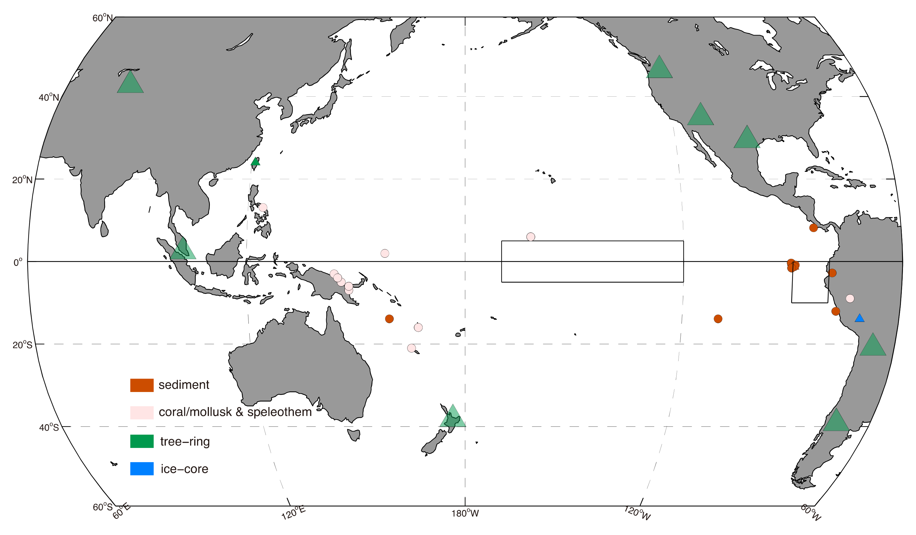
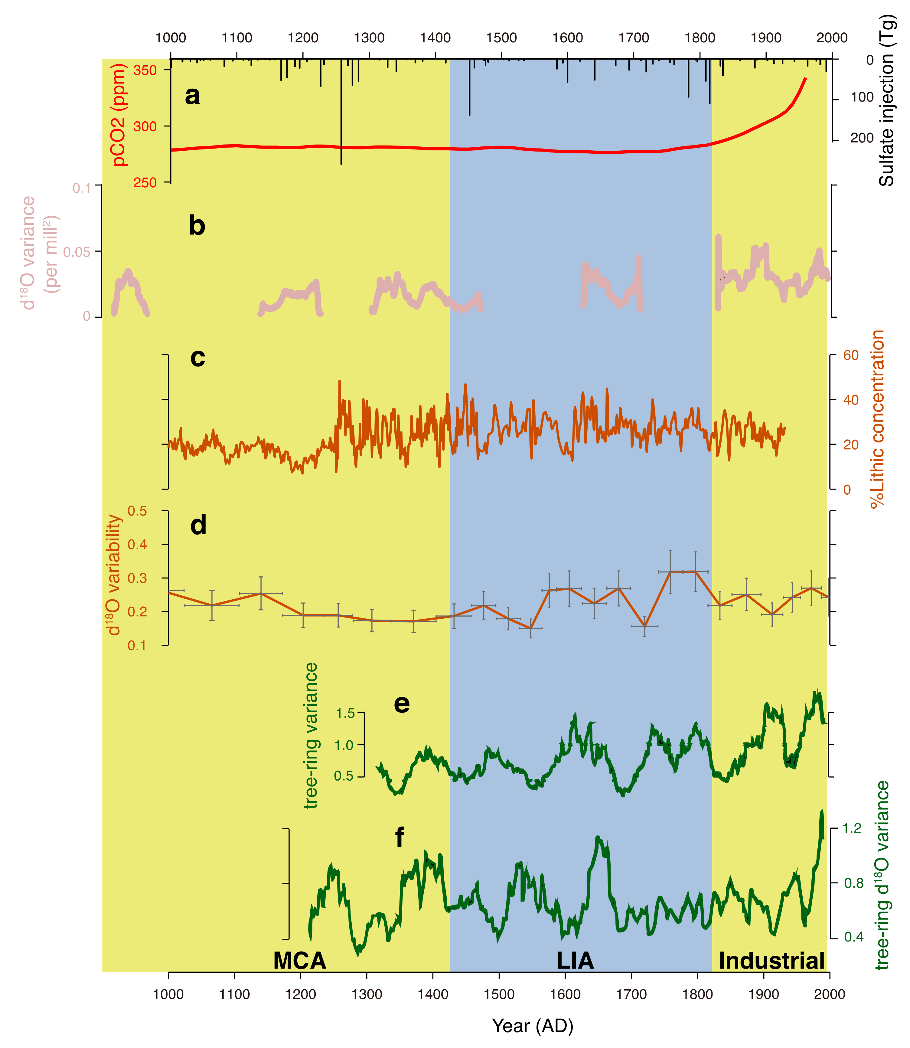
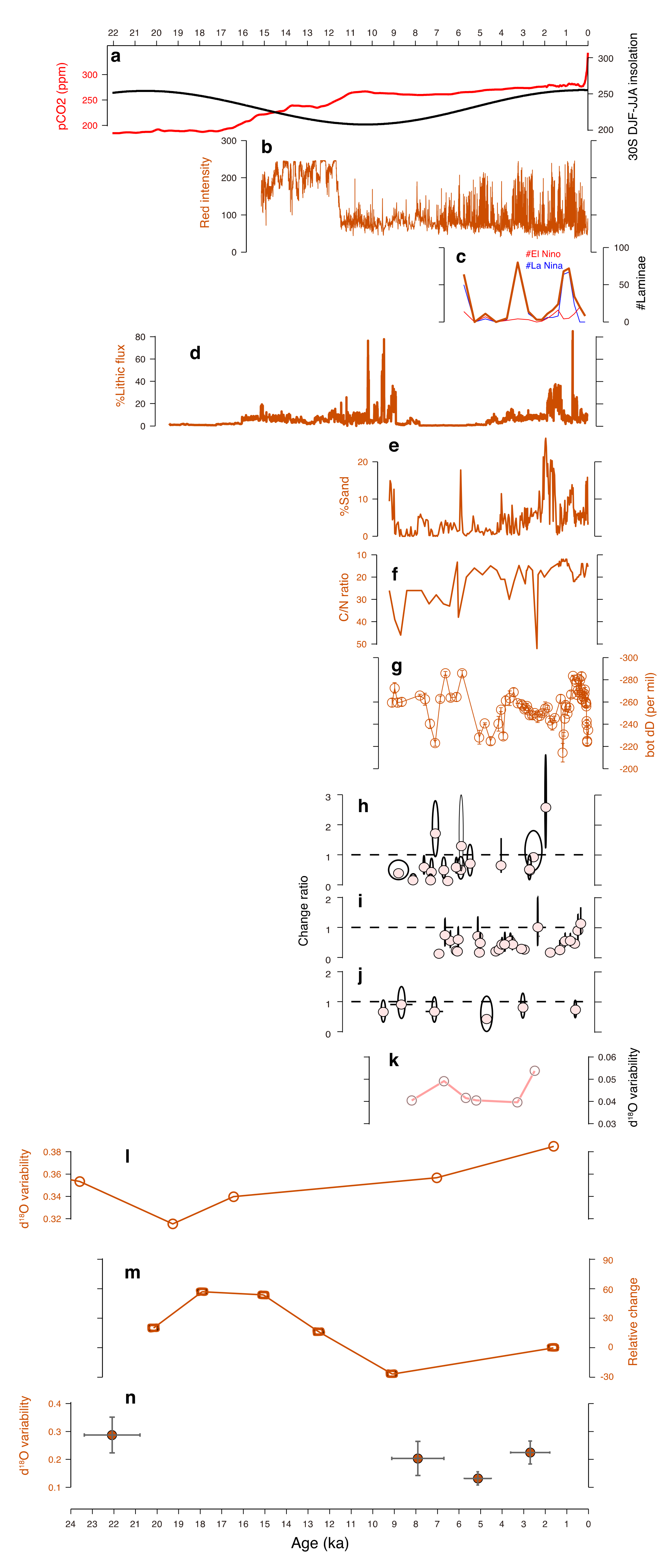
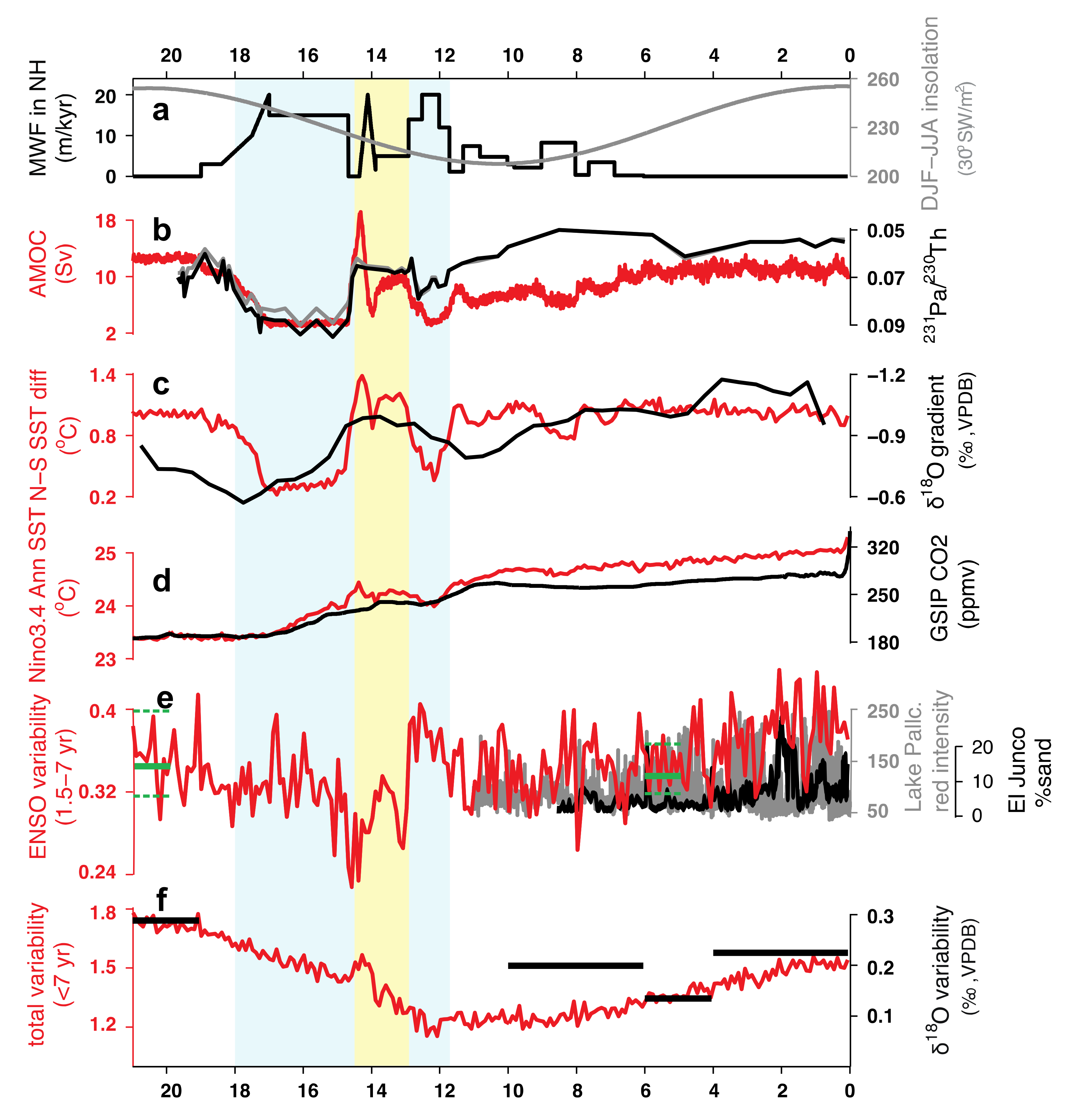
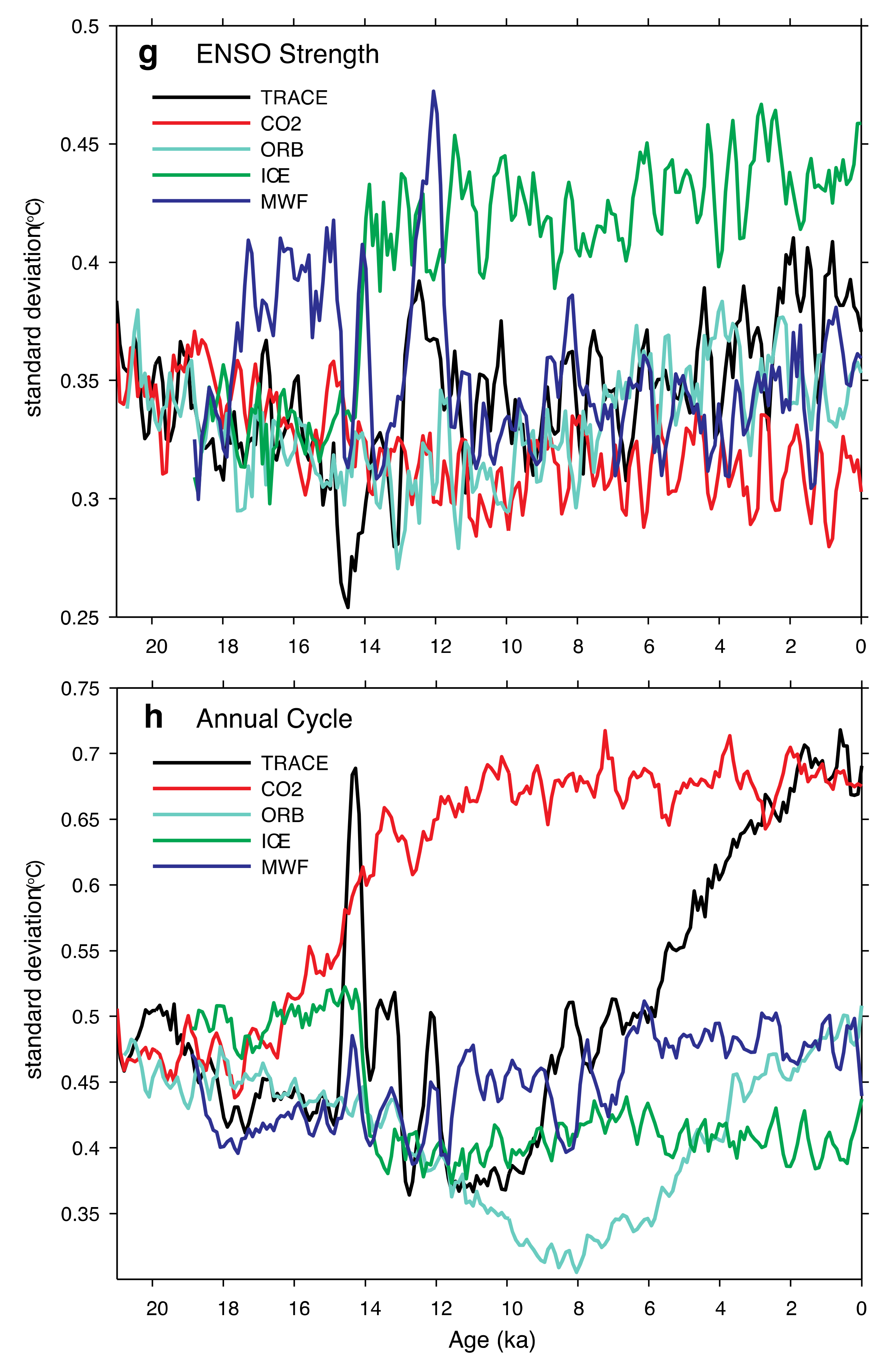
Table 1.
The list of paleo ENSO proxies.
| References | Type | Range | Location |
|---|---|---|---|
| Moy et al., 2002 [22] | Lake sediment | 10 ka | Laguna Pallcacocha, Ecuador |
| Riedinger et al., 2002 [23] | Lake sediment | 10 ka | Bainbridge Crater Lake, Galápagos Islands |
| Conroy et al., 2008 [24] | Lake sediment | 10 ka | El Junco Crater Lake, Galápagos Islands |
| Z. Zhang et al., 2014 [25] | Lake sediment | 10 ka | El Junco Crater Lake, Galápagos Islands |
| Thompson et al., 2017 [26] | Lake sediment | 10 ka | Bainbridge Crater Lake, Galápagos Islands |
| Rein et al., 2005 [27] | Marine sediment | 21 ka | 78° W, 12° S |
| Leduc et al., 2009 [28] | Marine sediment | 50 ka | 84° W, 8° N |
| Koutavas and Joanides, 2012 [29] | Marine sediment | 21 ka | 90° W, 1° S |
| Sadekov et al., 2013 [30] | Marine sediment | 21 ka | 90° W, 2° S |
| Ford et al., 2015 [31] | Marine sediment | 21 ka | 159° E, 14° S; 110° W, 14° S |
| Rustic et al., 2015 [32] | Marine sediment | 1 ka | 90° W, 1° S |
| Emile-Geay et al., 2015 [33] | Coral & Mollusk synthesis | 10 ka | WP, CP and EP clusters |
| Chen et al., 2016 [34] | speleothem | 10 ka | Northern Borneo, 4° N, 114° E |
| Watanabe et al., 2011 [35] | Coral | Pliocene | Philippines, 124° E, 13° N |
| Li et al., 2013 [36] | Tree-ring synthesis | 1 ka | 8 circum-Pacific clusters |
| Liu et al., 2017 [37] | Tree-ring isotope | 1 ka | Taiwan, 121° E, 24° N; 151° E, 24° N |
| Thompson et al., 2013 [38] | Ice-core | 1 ka | Quelccaya ice cap, 71° W, 14° S |
© 2018 by the authors. Licensee MDPI, Basel, Switzerland. This article is an open access article distributed under the terms and conditions of the Creative Commons Attribution (CC BY) license (http://creativecommons.org/licenses/by/4.0/).
Share and Cite
MDPI and ACS Style
Lu, Z.; Liu, Z.; Zhu, J.; Cobb, K.M. A Review of Paleo El Niño-Southern Oscillation. Atmosphere 2018, 9, 130. https://doi.org/10.3390/atmos9040130
AMA Style
Lu Z, Liu Z, Zhu J, Cobb KM. A Review of Paleo El Niño-Southern Oscillation. Atmosphere. 2018; 9(4):130. https://doi.org/10.3390/atmos9040130
Chicago/Turabian StyleLu, Zhengyao, Zhengyu Liu, Jiang Zhu, and Kim M. Cobb. 2018. "A Review of Paleo El Niño-Southern Oscillation" Atmosphere 9, no. 4: 130. https://doi.org/10.3390/atmos9040130
Note that from the first issue of 2016, this journal uses article numbers instead of page numbers. See further details here.