Reviewing Wind Measurement Approaches for Fixed-Wing Unmanned Aircraft

Abstract

One of the biggest challenges in probing the atmospheric boundary layer with small unmanned aerial vehicles is the turbulent 3D wind vector measurement. Several approaches have been developed to estimate the wind vector without using multi-hole flow probes. This study compares commonly used wind speed and direction estimation algorithms with the direct 3D wind vector measurement using multi-hole probes. This was done using the data of a fully equipped system and by applying several algorithms to the same data set. To cover as many aspects as possible, a wide range of meteorological conditions and common flight patterns were considered in this comparison. The results from the five-hole probe measurements were compared to the pitot tube algorithm, which only requires a pitot-static tube and a standard inertial navigation system measuring aircraft attitude (Euler angles), while the position is measured with global navigation satellite systems. Even less complex is the so-called no-flow-sensor algorithm, which only requires a global navigation satellite system to estimate wind speed and wind direction. These algorithms require temporal averaging. Two averaging periods were applied in order to see the influence and show the limitations of each algorithm. For a window of 4 min, both simplifications work well, especially with the pitot-static tube measurement. When reducing the averaging period to 1 min and thereby increasing the temporal resolution, it becomes evident that only circular flight patterns with full racetracks inside the averaging window are applicable for the no-flow-sensor algorithm and that the additional flow information from the pitot-static tube improves precision significantly.

1. Introduction

Atmospheric boundary layer (ABL) studies are increasingly complemented by in situ measurements using small unmanned aircraft systems (sUAS) [1,2,3,4,5,6,7,8]. Atmospheric sampling using sUAS dates back to 1961 [9] and has since been applied to atmospheric physics and chemistry [10,11,12,13], boundary-layer meteorology [14,15,16,17,18,19,20,21,22,23,24,25], and, more recently, also to wind-energy meteorology [26,27,28]. The capabilities of sUAS for meteorological sampling range from mean values for wind, thermodynamics, species concentration, etc., to highly resolved turbulence measurements, and from an accurate and diverse but larger sensor payload, down to small aircraft that can be operated from almost anywhere, with minimal logistical overhead. Elston et al. [29] provide details on the airframe parameters, estimation algorithms, sensors, and calibration methods, examining previous and current efforts for meteorological sampling with sUAS.

Usually, at least mean values, and often highly resolved measurements of an in situ wind vector, are crucial for the investigation or necessary for a deeper understanding of the turbulent atmosphere and turbulent atmospheric transport. The common method for measuring the 3D wind vector from research aircraft is a multi-hole probe in combination with the measured attitude, position, and velocity of the aircraft. In the following, this method is referred to as the multi-hole-probe algorithm (MHPA). The attitude is measured with an inertial measurement unit (IMU), position, and velocity of the aircraft using a global navigation satellite system (GNSS). The combination of both systems, usually supplemented by an extended Kalman filter (EKF), is called an inertial navigation system (INS). The wind vector is defined in the Earth coordinate system and equals the vector difference between the inertial velocity of the aircraft and the true airspeed of the aircraft. The MHPA is used in manned aircraft, as published by Lenschow [30], among others, and was adapted for sUAS by researchers, such as Van den Kroonenberg et al. [31], with the Mini Aerial Vehicle (M²AV) and by Wildmann et al. [32] using the Multi-purpose Airborne Sensor Carrier (MASC). The achievable high resolution and accuracy of this method demand a precise and fast INS, as well as pressure measurement with multi-hole probes. The study by de Jong et al. [33] introduced an algorithm (PTA, pitot tube algorithm) that does not require a multi-hole probe but only a pitot-static tube for dynamic pressure measurement, which makes it less complex and less expensive. Many common autopilot systems already use pitot-static tubes for airspeed measurement and are, without further instrumentation, capable of estimating the wind speed and direction. The study by Niedzielski et al. [34] also used this kind of approach with a consumer-grade sUAS. Unfortunately, there are no details on the algorithm documented. Even without a flow sensor aboard, the wind speed can be estimated using the ’no-flow-sensor’ algorithm (NFSA), as published by Mayer et al. [35]. With the sUAS SUMO (Small Unmanned Meteorological Observer, [36]), extensive measurements (e.g., [37]) were performed using this method. The NFSA uses only ground speed and flight path azimuth information from GNSS and is the least complex and least expensive method in this comparison. Bonin et al. [38] introduced variants of the NFSA and compared them with SODAR measurements, among others. Shuqing et al. [39] introduced the sUAS RPMSS (robotic plane meteorological sounding system) and uses a close variation of the NFSA to estimate the wind speed in their work.

This study provides an overview and review of the three methods and highlights the capabilities and limitations of these types of wind estimation methods that use sUAS. All introduced methods can be applied with the fully equipped sensor system which was used in this investigation. It includes a five-hole probe [40] and the INS IG500-N from SBG-Systems. The PTA can be examined using the INS data and only the tip hole of the five-hole probe for true airspeed measurement, and the NFSA can be investigated using only the GNSS data. Data sets from several measurement campaigns provide a variety of conditions for this comparison. The main factors of influence are the atmospheric conditions and the choice of flight paths. A representative selection with wind speeds between 2 and 15 m s${}^{-1}$, as well as various flight patterns, including horizontal straight and level segments (legs), circles, lying eights, and ascending racetracks for height profiles, were analyzed. Section 2 describes the measurement technology and the wind algorithms. Section 3 gives an overview of the experiments, Section 4 shows the results and discusses them, and Section 5 is the conclusion.

2. Methods and Measurement Techniques

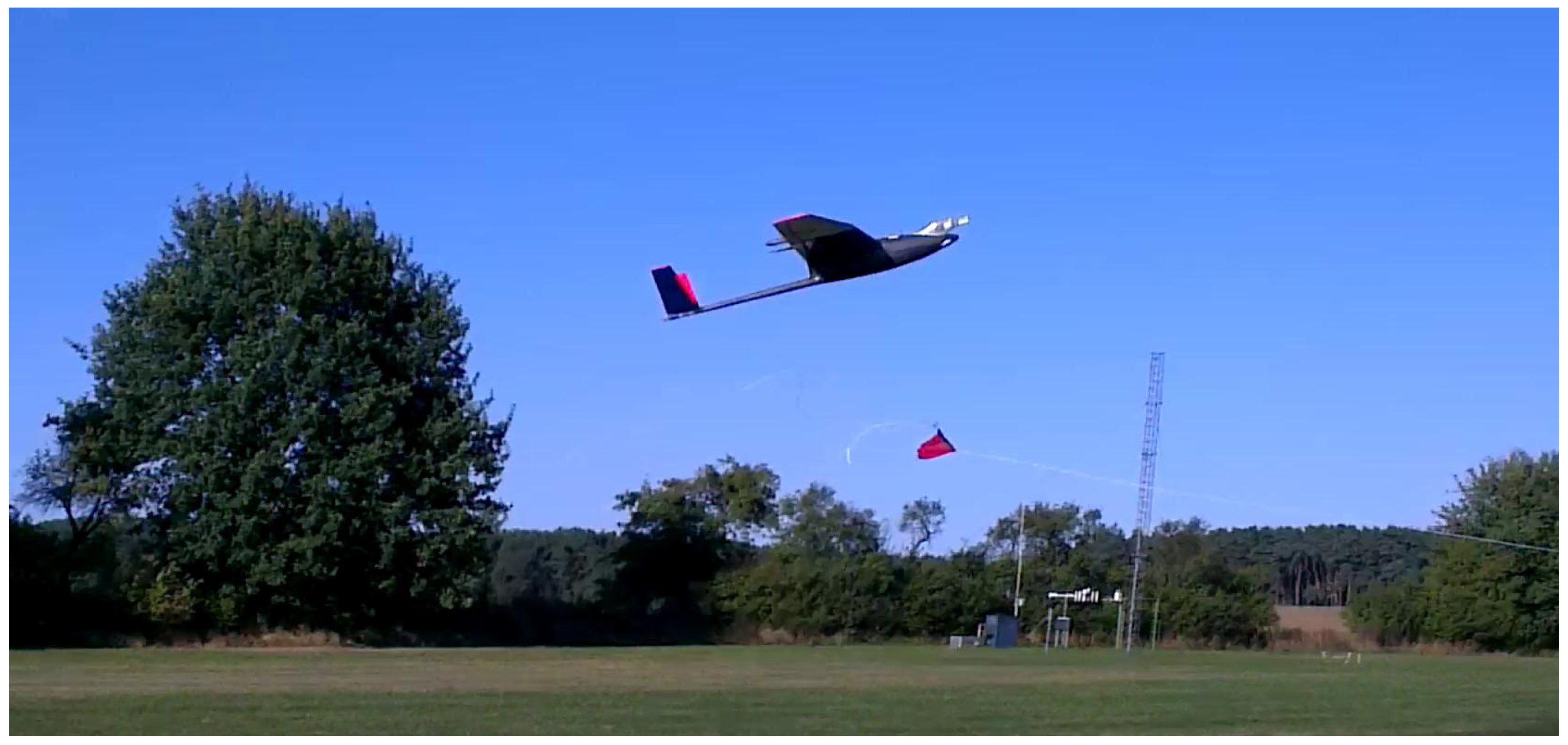
For atmospheric research, boundary-layer meteorology, and wind-energy studies, the environment-physics group at the Centre for Applied Geo-Science (ZAG), University of Tübingen, Germany, designed and built the research unmanned aerial vehicle (UAV) MASC (Figure 1). The MASC [32] is an electrically propulsed single engine (pusher) aircraft with a 3.5 m wing span. The total weight of the aircraft is 6 kg, including a 1 kg scientific payload. This sUAS is operated at an airspeed of 22 m s${}^{-1}$, as a trade-off between high spatial resolution of the measured data and gathering a snapshot of the atmosphere in a short time frame. The MASC operates fully automatically (except for landing and take-off). Height, flight path, and all other parameters of flight guidance are controlled by the autopilot system ROCS (Research Onboard Computer System) developed at the Institute of Flight Mechanics and Control (IFR) at the University of Stuttgart. The overall endurance of the MASC is 60 min or 80 km.

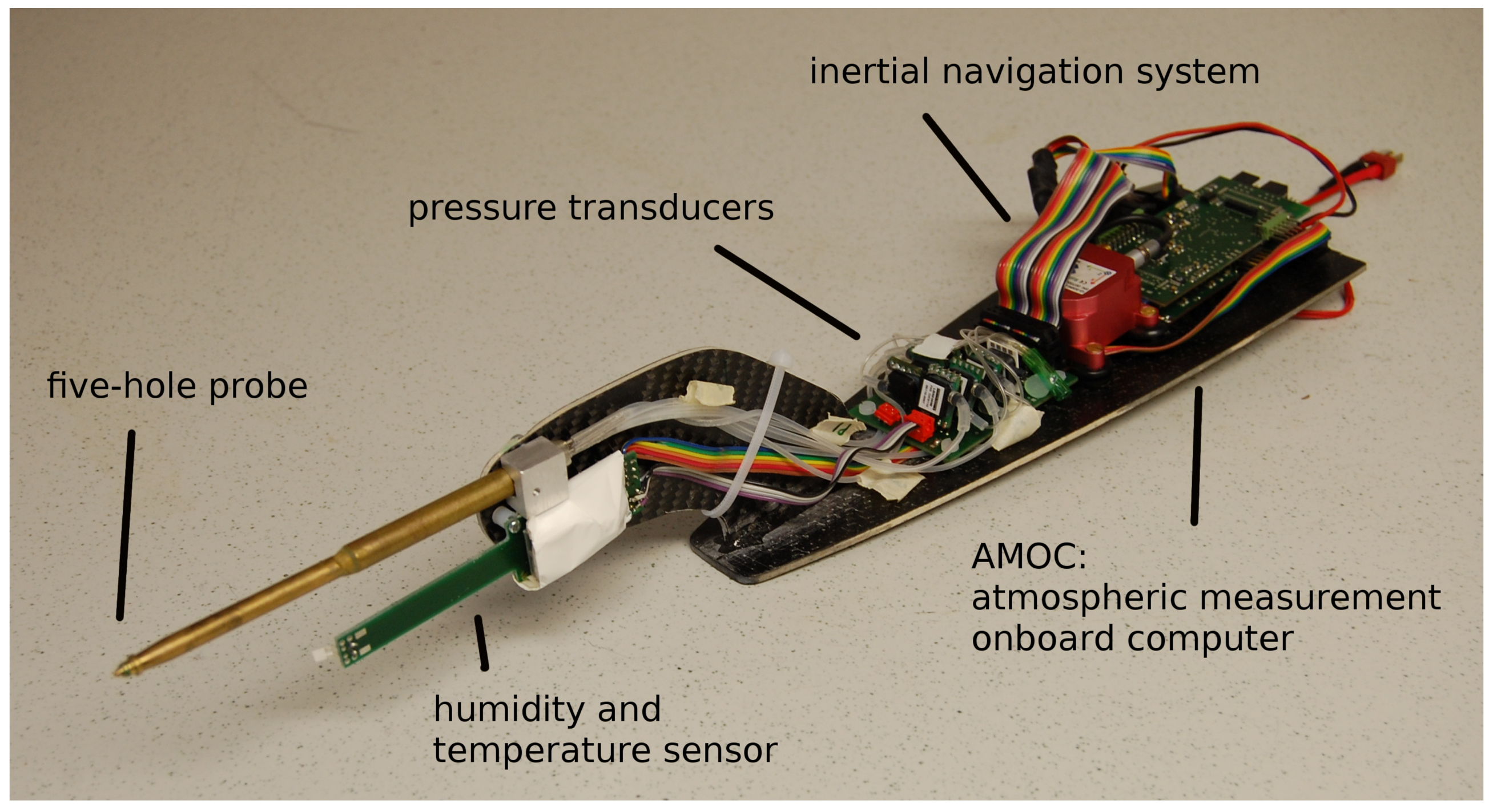
The scientific payload (Figure 2) for this investigation consists of several subsystems for measuring the 3D wind vector, air temperature, and water vapor. This includes a fast thermometer (fine wires, see [41]), a capacitive humidity sensor [32], a five-hole flow probe [31,40], and an INS. All sensors sample at 100 Hz and measure atmospheric turbulence. Considering the individual sensor inertia, a resolution of about 30 Hz (i.e., sub-meter resolution at 22 m s${}^{-1}$ airspeed, except for humidity, which is 3 Hz) is achieved. Thus, small turbulent fluctuations are resolved and the Nyquist theorem is fulfilled. The sensors and the data stream are controlled by the onboard measurement computer AMOC and stored at a 100 Hz rate. In order to watch the measurements online during flight, a data abstract is broadcasted to the ground station (standard laptop computer) at 1 Hz. The ground station also communicates with the autopilot. Changes in the flight plan are possible when the MASC is within a 5 km reach. Typical flight patterns with the MASC (these are common flight strategies for any research aircraft) are horizontal straight and level flights (so-called legs) both at constant height or stacked at various flight levels. These flight legs are used to calculate turbulence statistics, turbulent fluxes (e.g., [12,17]), spectra, and mean values, but they also measure the influence of surface heterogeneity and orography (complex terrain, e.g., [28]) on the lower atmosphere. The horizontal flights are usually supported by slanting flights that give data on the vertical profile of various atmospheric quantities, including the thermal stability (e.g., [42]). A combination of both (named the saw-tooth profile) returns both horizontal and vertical structures of the flow. For the sake of completeness, the star pattern or lying eights are commonly used to calibrate the MHPA method.

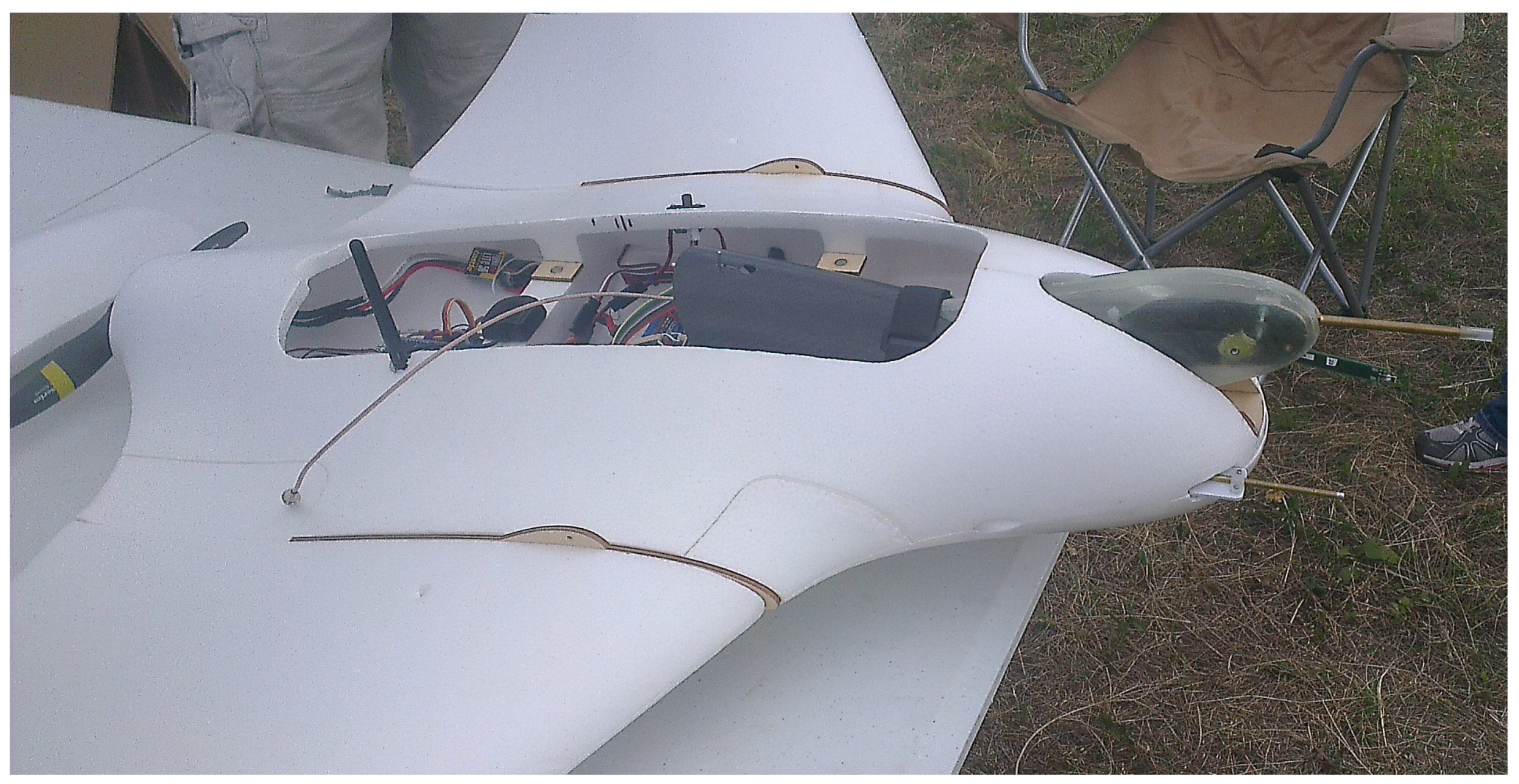
The standard sensor system developed for the MASC is self-sufficient and can be mounted on other airframes. To cover circular flight patterns, which are often used by flying wings like SUMO, or the return glider radiosonde (RGR, see [5]), data from a measurement campaign at the Boulder Atmospheric Observatory (BAO) were included: A commercially available flying wing (Skywalker X8) with a span of 2.1 m and a take-off weight of about 3.5 kg was equipped with the MASC sensor system and flown at the BAO. Figure 3 shows the Skywalker X8 flying wing with the sensor nose as used with the MASC. This sUAS is equipped with a Black Swift Technologies LLC (Boulder, CO , USA) autopilot system which maintains the airspeed, using a pitot-static tube, at 22 m s${}^{-1}$.

2.1. Coordinate Systems

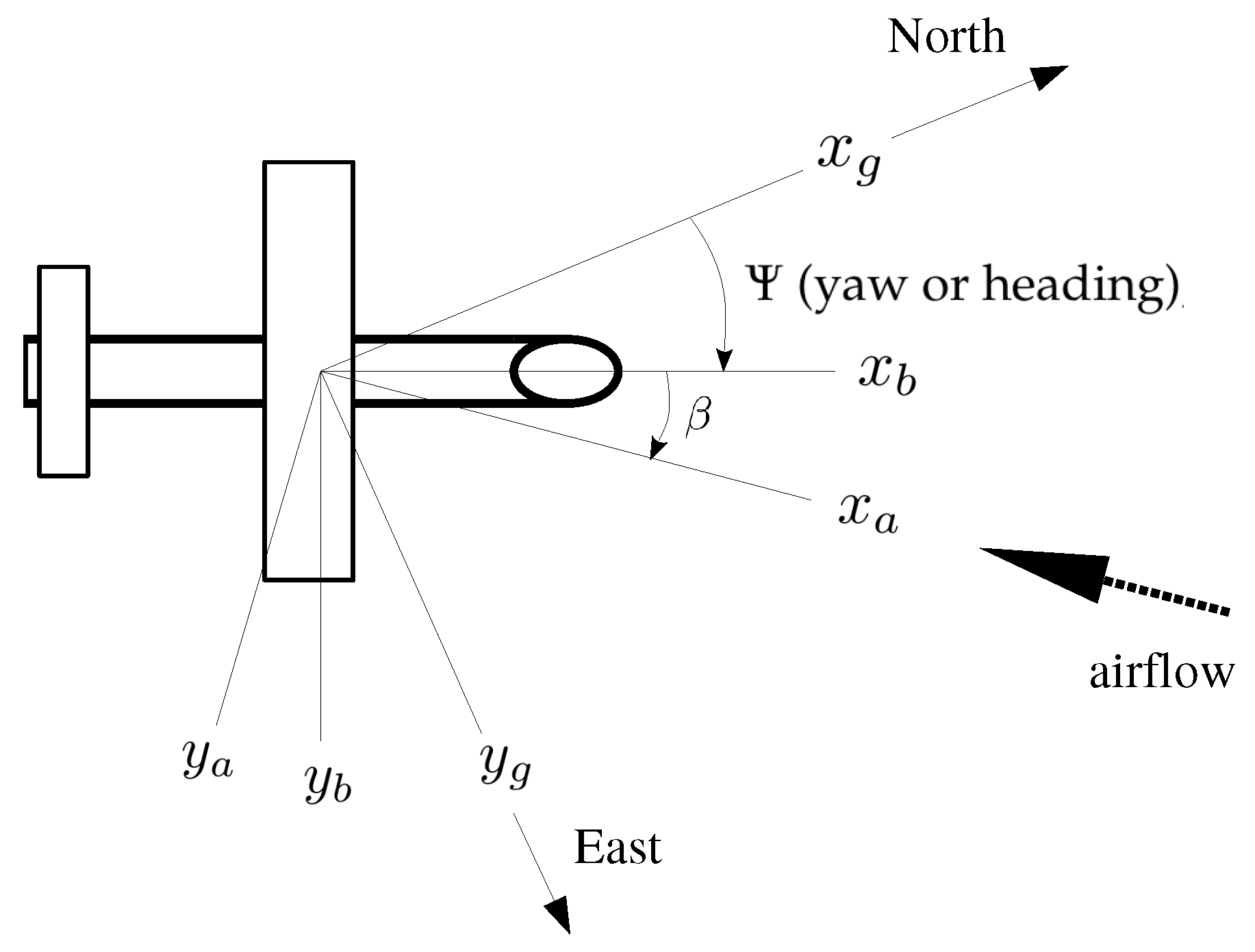
For the meteorological wind estimation, three Cartesian coordinate systems according to Boiffier [43] were used in the following, as shown in Figure 4. The first one is the Earth coordinate system or geodetic coordinate system with the index g. For example, the wind vector ${\overrightarrow{w}}_g$ in the geodetic coordinate system is defined by the vector components $w_x$ being positive northward, $w_y$ being positive eastward, and $w_z$ positive when facing downward. Furthermore, the body-fixed coordinate system of the aircraft with the index b was used. The origin is at the center of gravity of the aircraft; x faces forward, y faces starboard, and z faces downward. Besides that, the aerodynamic coordinate system, with the index a oriented by the aerodynamic velocity of the aircraft, was used. The aerodynamic coordinate system has the same origin as the body-fixed coordinate system and, with the angle of attack $\alpha$ (positive for air flow from below) and side slip $\beta$ (positive for flow from starboard), the aerodynamic coordinate system can be transformed into the aircraft coordinate system using the transformation ${\mathbf{T}}_{ba}$. Often, the wind vector ${\overrightarrow{w}}_m$ in meteorological coordinates (index m) instead of geodetic coordinates is used. The difference is a change in sign for the vertical component and a swapped first and second vector component. The meteorological wind vector ${\overrightarrow{w}}_m$ can be calculated using the transformation ${\mathbf{T}}_{mg}$ with

$${\overrightarrow{w}}_m={\mathbf{T}}_{mg}{\overrightarrow{w}}_g=\left(\begin{array}{ccc}0& 1& 0\\ 1& 0& 0\\ 0& 0& -1\end{array}\right)\left(\begin{array}{c}{w}_x\\ w_y\\ w_z\end{array}\right)$$

(1)

However, in this study, only the wind vector ${\overrightarrow{w}}_g$ in the geodetic coordinate system was used.

2.2. Wind Vector Estimation

The wind vector $\overrightarrow{w}$ is the orientation and magnitude of the airflow. A nonstationary observer (e.g., an sUAS) sees the relative velocity $\overrightarrow{u}$ only, and from a fixed point of view (e.g., the Earth coordinate system), the observer is moving with a resulting velocity $\overrightarrow{v}$ that is the sum of $\overrightarrow{u}$ and $\overrightarrow{w}$. This fundamental relation is the basis of all wind measurement techniques with fixed-wing aircraft. The wind vector ${\overrightarrow{w}}_g$ in the geodetic coordinate system is the difference between ${\overrightarrow{v}}_g$ and ${\overrightarrow{u}}_g$. The velocity vector ${\overrightarrow{v}}_g$ of the sUAS is generally estimated with GNSS data and can be measured at a good accuracy with consumer-grade GNSS receivers, whereas the true airspeed vector ${\overrightarrow{u}}_g$ relative to the sUAS represents a more challenging parameter to obtain for any wind measurement technique of a fixed-wing sUAS, as well as the attitude (Eulerian angles) of the aircraft. The wind vector ${\overrightarrow{w}}_g$ has to be calculated (according to, e.g., Bange [44]) using

$${\overrightarrow{w}}_g={\overrightarrow{v}}_g+{\mathbf{T}}_{gb}\left({\overrightarrow{u}}_b+{\overrightarrow{\Omega }}_b\times \overrightarrow{L}\right)$$

(2)

with the true airspeed vector ${\overrightarrow{u}}_b$ in the body-fixed coordinate system of the aircraft, and the transformation matrix ${\mathbf{T}}_{gb}$ in the geodetic coordinate system. The vector of angular body rates ${\overrightarrow{\Omega }}_b$ and its lever arm $\overrightarrow{L}$ describe the effect due to the spatial separation between INS and the multi-hole probe and can be (according to [45]) neglected since the lever arm $\overrightarrow{L}$ is only a few centimeters in our sUAS. Two fundamental approaches to measuring the true airspeed vector are possible. Either the true airspeed vector ${\overrightarrow{u}}_a$ of the sUAS in the aerodynamic coordinate system can be measured and transformed into geodetic coordinates, or the true airspeed vector ${\overrightarrow{u}}_g$ in the geodetic coordinate system is derived from the changes in ${\overrightarrow{v}}_g$ under the assumption of constant wind speed and direction. The first approach can be seen as the direct measurement, given that the relative wind vector and the position and attitude of the aircraft need to be measured. If these quantities are measured quickly and precisely, small wind vector fluctuations are resolved in time and space and turbulent fluxes, among other factors, can be calculated. If one of the quantities for the direct measurement is missing, assumptions have to be made to compensate for that, and averaging along the flight path is necessary. Summarizing, the MHPA method is the direct approach to solving Equation (2), with expected uncertainties that can be calculated through the propagation of sensor uncertainties [31], while both the PTA and NFSA methods estimate the wind vector, which is also averaging over a certain period. Averaged data do not allow for turbulent flux calculations, in general. Furthermore, the tuning of the autopilot and the aerodynamic design of the aircraft can influence the wind measurement, but this cannot be analyzed in the scope of this study.

2.2.1. Multi-Hole-Probe Wind Algorithm (MHPA)

Through measurements of a multi-hole probe, the true airspeed, side slip angle, and angle of attack are retrieved, which can be used to rotate the airspeed vector to the body-fixed coordinate system and, with the transformation ${\mathbf{T}}_{ba}$, it can be written as

$${\overrightarrow{w}}_g={\overrightarrow{v}}_g+{\mathbf{T}}_{gb}{\mathbf{T}}_{ba}{\overrightarrow{u}}_a$$

(3)

The true airspeed vector ${\overrightarrow{u}}_a$ in the aerodynamic coordinate system cannot be measured directly and requires intensive calibration of the multi-hole probes in the wind tunnel. The norm $|{\overrightarrow{u}}_a|$ is calculated with the total air temperature $T_{\mathrm{tot}}$, which is assumed to be adiabatically stagnated on the probe’s tip, and the static pressure p, as well as the dynamic pressure increment q. These quantities are the outcome of normalized pressure differences between the pressure holes on the multi-hole probe and the wind tunnel calibration.

$$|{\overrightarrow{u}}_a{|}^2=2c_p{T}_{\mathrm{tot}}\left[1-{\left(\frac{p}{p+q}\right)}^{\kappa }\right]$$

(4)

The Poisson number is defined by $\kappa =R{c_p}^{-1}$, with $R=287$ J kg${}^{-1}$ K${}^{-1}$ being the gas constant for dry air and $c_p=1004$ J kg${}^{-1}$ K${}^{-1}$ the specific heat of dry air. In our study, this was done for a five-hole probe according to Bange [44]. The true airspeed vector ${\overrightarrow{u}}_a$ must be transformed from the aerodynamic coordinate system into the body-fixed coordinate system using ${\mathbf{T}}_{ba}$ with the angle of attack $\alpha$ (positive for air flow from below) and side slip $\beta$ (positive for flow from starboard). Since $\alpha$ and $\beta$ are determined by the calibration procedure in the wind tunnel, there is a small difference between the body-fixed coordinate system of the sUAS and the experimental coordinate system in the wind tunnel due to the calibration procedure. According to Bange [44], this can be neglected for small angles. The true airspeed vector in the body-fixed coordinate system is:

$${\overrightarrow{u}}_b=-\frac{|{\overrightarrow{u}}_a|}{\sqrt{1+{tan}^2\alpha +{tan}^2\beta }}\left(\begin{array}{c}1\\ tan\beta \\ tan\alpha \end{array}\right),$$

(5)

With ${\mathbf{T}}_{gb}$, which consists of three sequential turnings, the coordinate system is transformed from body-fixed into geodetic (index g) coordinates. ${\mathbf{T}}_1(\Phi )$ defines rolling about $x_b$, ${\mathbf{T}}_2(\Theta )$ defines pitching about $y_b$, and ${\mathbf{T}}_3(\Psi )$ defines yawing about $z_b$. Then,

$$\begin{array}{cc}\hfill {\mathbf{T}}_{gb}& ={\mathbf{T}}_1(\Phi ){\mathbf{T}}_2(\Theta ){\mathbf{T}}_3(\Psi )\hfill \\ & =\left(\begin{array}{ccc}1& 0& 0\\ 0& cos\Phi & -sin\Phi \\ 0& sin\Phi & cos\Phi \end{array}\right)\left(\begin{array}{ccc}cos\Theta & 0& sin\Theta \\ 0& 1& 0\\ -sin\Theta & 0& cos\Theta \end{array}\right)\left(\begin{array}{ccc}cos\Psi & -sin\Psi & 0\\ sin\Psi & cos\Psi & 0\\ 0& 0& 1\end{array}\right)\hfill \end{array}$$

(6)

In accordance with methods previously described in [44], among other authors, and with the Euler angles measured by the INS, the wind vector ${\overrightarrow{w}}_g$ can be calculated. Together with $D=\sqrt[]{1+{tan}^2\beta +{tan}^2\alpha }$ and the Euler angles $\Phi$ (roll), $\Theta$ (pitch), and $\Psi$ (yaw or heading), Equation (2) can be written with the wind vector in the geodetic coordinate system:

$$\begin{array}{cc}\hfill \overrightarrow{w_g}& =\overrightarrow{v_g}\hfill \\ & -\frac{|{\overrightarrow{u}}_a|}{D}\left(\begin{array}{c}cos\Psi cos\Theta +tan\alpha (sin\Phi sin\Psi +cos\Phi cos\Psi sin\Theta )+tan\beta (cos\Psi sin\Phi sin\Theta -cos\Phi sin\Psi )\\ cos\Theta sin\Psi +tan\alpha (cos\Phi sin\Psi sin\Theta -cos\Psi sin\Phi )+tan\beta (cos\Phi cos\Psi +sin\Phi sin\Psi sin\Theta )\\ -sin\Theta +cos\Phi cos\Theta tan\alpha +cos\Theta sin\Phi tan\beta \end{array}\right)\hfill \end{array}$$

(7)

Lenschow and Spyers-Duran [46] introduced a simplified version of Equation (7), using small-angle approximations for the measurement taken with manned aircraft during straight level flights. Calmer et al. [47] also applied this formulation to their vertical wind velocity measurements with sUAS. Since there is no benefit when applying these simplifications, other than a shorter formulation of the equation and a lower computational effort, the authors do not recommend using these simplifications for sUAS. For a manned aircraft, the inertia of mass is several orders of magnitude higher and, therefore, the movement of the aircraft in turbulence is less. Especially because there is no substantial benefit of such simplifications and because an investigation would need different methods from those in this study, simplifications were not considered.

2.2.2. The Pitot Tube Algorithm (PTA)

The PTA uses INS data and highly reduced flow information compared to the MHPA described in Section 2.2.1. A singular pitot-static tube in the nose of the aircraft is used. The PTA has a similar approach to that of the MHPA but needs temporal averaging to compensate for the missing information concerning the perpendicular vector components of the airspeed on the aircraft. Starting from Equation (2), the wind vector equals the vector difference between the ground speed of the sUAS and the true airspeed vector, whereas, when dissociated from the direct measurement, the airspeed of the sUAS can only be approximated with the pitot-static tube. The calculation of ${\overrightarrow{u}}_q$ is done in the simplest way by using the stagnation pressure and Bernoulli’s principle for incompressible flows. For example, with a pitot-static tube, the first vector component of $u_{qx}=\sqrt{2d{p}_0/\rho }$ is calculated. The other components remain as unknowns in the algorithm of de Jong et al. [33].

$$\overrightarrow{u_q}=\left(\begin{array}{c}\sqrt{2d{p}_0/\rho }\\ u_{qy}\\ u_{qz}\end{array}\right)$$

(8)

The pitot-static tube is mounted so it is aligned with $x_b$ in the aircraft coordinate system (see also Figure 4). In opposition to the formulation in Section 2.2.1 for the MHPA and to highlight the differences, the nomenclature for the estimated true airspeed vector used for the PTA is ${\overrightarrow{u}}_q$. Only the lateral component of the true airspeed vector ${\overrightarrow{u}}_q$ is estimated, and misalignments between the aerodynamic and the aircraft coordinate systems cannot be considered. The estimated true airspeed vector ${\overrightarrow{u}}_q$ is assumed to be aligned with $x_b$ and the transformation ${\mathbf{T}}_{ba}$ in Equation (3) is therefore neglected, and only the coordinate transformation ${\mathbf{T}}_{gb}$ from body-fixed to geodetic coordinates is performed.

$$\overrightarrow{w_g}=\overrightarrow{v_g}+{\mathbf{T}}_{gb}\overrightarrow{u_q}$$

(9)

Since the misalignment between the aerodynamic and the aircraft coordinate system cannot be considered, the true airspeed vector ${\overrightarrow{u}}_q$ in Equation (8) is referenced in body-fixed coordinates (see also Figure 4), with the origin at the center of gravity; x is along the fuselage and is positive when facing forward, y is positive when facing starboard, and z is positive when facing upward. Comparing Equation (8) for the PTA with Equation (5) for the MHPA, the differences in the true airspeed measurement are obvious. The PTA can give a precise estimate of the true airspeed only if $\alpha =\beta =0$ and, therefore, the norm $|{\overrightarrow{u}}_q|$ is generally underestimated by the PTA. For this comparison, we simulated a pitot-static tube with our five-hole probe by using the pressure reading between the central hole of the five-hole probe and the static port just behind the probe tip. This represents a rather simple implementation of a standard pitot-static tube, which is reasonable for estimating the wind speed with the PTA and its expected precision. To calculate a solution using these measurements, the PTA needs reordering of the variables in Equations (8) and (9) and an averaging over a certain number of time steps. The measured quantities ${\overrightarrow{v}}_g$ and $u_{qx}$ are separated from the unknowns, which are the wind vector ${\overrightarrow{w}}_g$ and the other vector components $u_{qy}$ and $u_{qz}$ of the true airspeed. The emerging system of equations becomes overdetermined when adjoining further measurements, defined by i, and the solution is calculated by solving, over one time step, a window of size M. To be able to separate the knowns and unknowns, Equation (9) is written in vector notation, using the vector components ${\overrightarrow{v}}_g=(v_x,v_y,v_z)$ and ${\overrightarrow{w}}_g=(w_x,w_y,w_z)$. The transformation matrix ${\mathbf{T}}_{gb}$ (see also Equation (6)) is split up into its elements by

$$\begin{array}{cc}\hfill {\mathbf{T}}_{gb}& =\left[\begin{array}{ccc}{T}_{1x}& T_{1y}& T_{1z}\\ T_{2x}& T_{2y}& T_{2z}\\ T_{3x}& T_{3y}& T_{3z}\end{array}\right]\hfill \\ & =\left[\begin{array}{ccc}cos\Theta cos\Psi & sin\Phi sin\Theta cos\Psi -cos\Phi sin\Psi & cos\Phi sin\Theta cos\Psi +sin\Phi sin\Psi \\ cos\Theta sin\Psi & sin\Phi sin\Theta sin\Psi +cos\Phi cos\Psi & cos\Phi sin\Theta sin\Psi -sin\Phi cos\Psi \\ -sin\Theta & sin\Phi cos\Theta & cos\Phi cos\Theta \end{array}\right]\hfill \end{array}$$

(10)

and Equations (8) and (9) become

$$\begin{array}{cc}\hfill \left[\begin{array}{c}{w}_x\\ w_y\\ w_z\end{array}\right]=& \left[\begin{array}{c}{v}_x\\ v_y\\ v_z\end{array}\right]+\left[\begin{array}{c}{T}_{1x}{u}_{qx}+T_{1y}{u}_{qy}+T_{1z}{u}_{qz}\\ T_{2x}{u}_{qx}+T_{2y}{u}_{qy}+T_{2z}{u}_{qz}\\ T_{3x}{u}_{qx}+T_{3y}{u}_{qy}+T_{3z}{u}_{qz}\end{array}\right]\hfill \end{array}$$

(11)

The equation is rewritten to separate the knowns from the unknowns,

$$\begin{array}{c}\hfill v_x+T_{1x}{u}_{qx}=w_x-T_{1y}{u}_{qy}-T_{1z}{u}_{qz}\\ \hfill v_y+T_{2x}{u}_{qx}=w_y-T_{2y}{u}_{qy}-T_{2z}{u}_{qz}\\ \hfill v_z+T_{3x}{u}_{qx}=w_z-T_{3y}{u}_{qy}-T_{3z}{u}_{qz}\end{array}$$

(12)

and the knowns can be aggregated in ${\eta }_k$. For every directional component $k\in \{x,y,z\}$, the three equations are:

$$\begin{array}{cc}\hfill {\eta }_k=v_k+T_{1k}{u}_{qx}& =w_k-T_{2k}{u}_{qy}-T_{3k}{u}_{qz}\hfill \end{array}$$

(13)

Assuming that ${\overrightarrow{w}}_g$ is temporally and spatially constant along the window of size M, the k Equation (13) can be combined with a linear independent system of equations. With every measurement point i, two new unknowns ($u_{qy}^{(i)}$ and $u_{qz}^{(i)}$) accrue to the system.

$$\begin{array}{cc}\hfill \left[\begin{array}{c}{\eta }_x^{(1)}\\ {\eta }_y^{(1)}\\ {\eta }_z^{(1)}\\ {\eta }_x^{(2)}\\ {\eta }_y^{(2)}\\ {\eta }_z^{(2)}\\ ⋮\\ {\eta }_x^{(N)}\\ {\eta }_y^{(N)}\\ {\eta }_z^{(N)}\end{array}\right]& =\left[\begin{array}{cccccccccc}1& 0& 0& -T_{1y}^{(1)}& -T_{1z}^{(1)}& 0& 0& \cdots & 0& 0\\ 0& 1& 0& -T_{2y}^{(1)}& -T_{2z}^{(1)}& 0& 0& \cdots & 0& 0\\ 0& 0& 1& -T_{3y}^{(1)}& -T_{3z}^{(1)}& 0& 0& \cdots & 0& 0\\ 1& 0& 0& 0& 0& -T_{1y}^{(2)}& -T_{1z}^{(2)}& \cdots & 0& 0\\ 0& 1& 0& 0& 0& -T_{2y}^{(2)}& -T_{2z}^{(2)}& \cdots & 0& 0\\ 0& 0& 1& 0& 0& -T_{3y}^{(2)}& -T_{3z}^{(2)}& \cdots & 0& 0\\ ⋮& ⋮& ⋮& ⋮& ⋮& ⋮& ⋮& \ddots & ⋮& ⋮\\ 1& 0& 0& 0& 0& 0& 0& \cdots & -T_{1y}^{(M)}& -T_{1z}^{(M)}\\ 0& 1& 0& 0& 0& 0& 0& \cdots & -T_{2y}^{(M)}& -T_{2z}^{(M)}\\ 0& 0& 1& 0& 0& 0& 0& \cdots & -T_{3y}^{(M)}& -T_{3z}^{(M)}\end{array}\right]\left[\begin{array}{c}{w}_x\\ w_y\\ w_z\\ u_{qy}^{(1)}\\ u_{qz}^{(1)}\\ u_{qy}^{(2)}\\ u_{qz}^{(2)}\\ ⋮\\ u_{qy}^{(M)}\\ u_{qz}^{(M)}\end{array}\right]\hfill \end{array}$$

(14)

The unknowns n and the number of equations m have the relation $n=3+\frac{2}{3}m$ and, therefore, starting from a window size of $M=3$, the system of equations is solvable. In practice, the system of equations needs to be explicitly overdetermined to average over small-scale fluctuations in the wind field and obtain a solid mean wind. If the difference between $v_g$ and $u_g$ remains unchanged during the averaging period, the matrix is close to singular. For this reason, some variation in flight direction is essential for the algorithm. Equation (14) is solved numerically for $w_x,w_y,$ and $w_z$ with the least square method. The obtained wind vector ${\overrightarrow{w}}_g$ in the geodetic coordinate system is the best fit for the i measurements inside the averaging window M. It must be noted that the PTA cannot provide a vertical wind component $w_z$ with reasonable uncertainty, at least for the presented flight pattern. Given that pitch angles $\theta$ are generally small in the presented flights, the vertical component of the airspeed measurements ($T_{3x}{u}_{qx}$ in Equation (12)) will be small, which leads to high uncertainties if errors are propagated through the PTA for the vertical wind component. Additionally, the long averaging periods that are necessary for the PTA will average over the most significant small-scale vertical motions.

2.2.3. The No-Flow-Sensor Algorithm (NFSA)

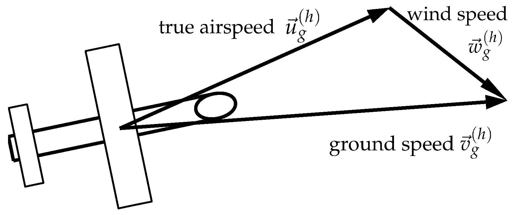
Imagining an aircraft flying horizontal circles in a constant wind field, it is evident that the ground speed is dependent on the angle between the wind direction and the flight path. Figure 5 shows the vector sum of the horizontal ground speed ${\overrightarrow{v}}_g^{(h)}$, the horizontal true airspeed ${\overrightarrow{u}}_g^{(h)}$, and the horizontal wind speed ${\overrightarrow{w}}_g^{(h)}$, which are used for the NFSA. The ground speed of the aircraft is minimal when flying directly against the wind and is maximal vice versa. It is presumed that the airspeed of the aircraft is constant; for the MASC and the Skywalker X8, this is assured by the autopilot systems. Applying a constant throttle and/or pitch rate to keep a constant airspeed makes the application of the NFSA even easier since the autopilot does not even require a pitot-static tube. This approach is followed with the SUMO, among other systems. Differences between these flight guidance approaches (constant throttle and/or pitch rate setting of the autopilot or an autopilot with pitot-static tube) to keep a constant airspeed can be neglected for this comparison since they are insignificant when averaging over the window M.

Starting from Equation (2), according to Mayer et al. [35], the mean norm of the horizontal true airspeed ${\overrightarrow{u}}_g^{(h)}$ inside the window M is related to the difference in the horizontal ground speed ${\overrightarrow{v}}_g^{(h)}$ and the horizontal wind speed ${\overrightarrow{w}}_g^{(h)}$, using the geodetic coordinate system as a reference.

$$\begin{array}{cc}\hfill |\overline{{\overrightarrow{u}}_g^{(h)}}|& =\frac{1}{M}\sum _i^M|{\overrightarrow{v}}_{gi}^{(h)}-{\overrightarrow{w}}_g^{(h)}|\hfill \end{array}$$

(15)

where M is the number of measurement points in the averaging window, and the method presumes that the aircraft is flying at constant airspeed and assumes that the wind speed is constant. Therefore, the components on each side of Equation (15) must level each other out for every measurement i. To deal with fluctuations in the wind field and to solve for the horizontal wind speed, Equation (15) is reordered and the variance ${\sigma }^2$ of the measurements in the window M is introduced:

$$\begin{array}{cc}\hfill {\sigma }^2& =\frac{1}{M}\sum _i^M{\left(|{\overrightarrow{v}}_{gi}^{(h)}-{\overrightarrow{w}}_g^{(h)}|-|\overline{{\overrightarrow{u}}_g^{(h)}}|\right)}^2\hfill \end{array}$$

(16)

To calculate the horizontal wind speed from Equation (16), the smallest possible value for the variance is approximated numerically using the downhill-simplex method according to McKinnon [48]. More details can be found in Mayer et al. [35].

3. Experiments

The wind field and turbulence of the atmospheric boundary layer and the choice of flight paths are the main factors to argue the potential differences between these wind estimation algorithms. A representative pick from four measurement campaigns with wind speeds between 2 and 15 m s${}^{-1}$, as well as various flight patterns, including horizontal straight flight legs, circles, lying eights, and ascending racetracks for height profiles, were selected. A brief description of the prevailing atmospheric conditions is also gathered in

Table 1. Flight sections with location, date, and duration in local time, pattern, and brief atmospheric condition.

Location	Date	From	Until	Flight Path	Condition
Boulder (BAO)	8 August 2014	3:12 p.m.	3:35 p.m.	circular	weakly convective
Schnittlingen (SNT)	7 May 2015	11:23 a.m.	11:51 a.m.	horizontal racetracks	sheared flow
Helgoland (HEL)	10 October 2014	9:20 a.m.	9:51 a.m.	ascending racetracks	strong wind
Pforzheim (PFR)	11 July 2013	9:50 a.m.	10:08 a.m.	lying eight, long straights	convective

.

To compare the performance of the three methods MHPA, PTA, and NFSA and to highlight limitations, two averaging periods M were chosen in this study and applied to all experiments. The long averaging period is $M=240$ s and acts in accordance with the experiment in Pforzheim (PFR), where the longest racetracks were performed. $M=240$ s comprised two racetracks in PFR. The short averaging period is $M=60$ s and comprises two circles for the shortest racetracks at the BAO.

3.1. Boulder Atmospheric Observatory (BAO)

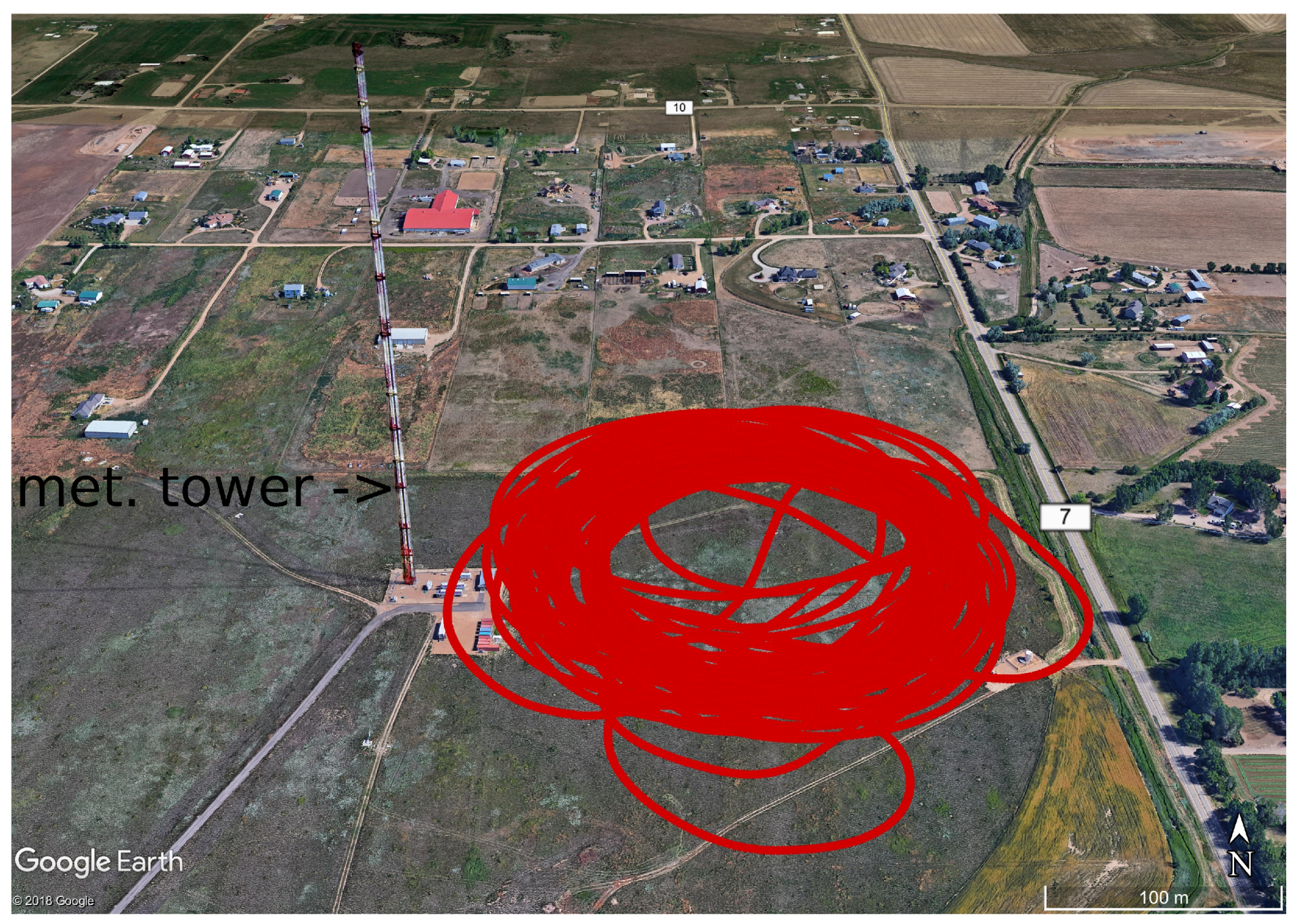
The Boulder Atmospheric Observatory (BAO) was a test facility of the National Oceanic and Atmospheric Administration (NOAA) in the USA. It was located in the state of Colorado at around 1580 m above sea level. The flight took place on 8 August in 2014 and the presented data fraction was measured between 3:12 and 3:35 p.m. local time. The wind was ≈2 m s${}^{-1}$ from the east. This data was measured with the Skywalker X8 flying wing (see also Section 2) performing fixed-radius circles (Figure 6) at a constant height of 100 m above ground level (AGL) and with an airspeed of 22 m s${}^{-1}$. A full circle takes about half a minute. This is a typical pattern [35] when using the NFSA for wind speed and direction estimation. To ensure a sufficient quantity of data, a period of 43 consecutive circles was chosen.

For this flight, data from a meteorological tower with a resolution of 1 min, located northeast of the circular flight path, was available for comparison. The tower is visible in Figure 6, and the data measured by the aircraft and the tower is shown in

Table 2. Horizontal wind speed and wind direction at Boulder Atmospheric Observatory meteorological tower. Data at 100 m above ground level (AGL) in comparison with the multi-hole-probe algorithm (MHPA) for the flight on 8 August 2014 between 3:12:06 p.m. and 3:34:36 p.m. local time. Additionally, the data is divided into three intervals of 450 s each.

	3:12:06 p.m. Until 3:34:36 p.m.	First 450 s	Second 450 s	Last 450 s
Tower BAO	$2.02\pm 0.26$ m s${}^{-1}$	$2.18\pm 0.31$ m s${}^{-1}$	$2.01\pm 0.16m{s}^{-1}$	$1.87\pm 0.19m{s}^{-1}$
	$68\pm {21}^{\circ }$	$93\pm 8^{\circ }$	$57\pm {11}^{\circ }$	$52\pm 7^{\circ }$
MHPA BAO	$2.25\pm 0.24$ m s${}^{-1}$	$2.39\pm 0.06$ m s${}^{-1}$	$2.16\pm 0.14$ m s${}^{-1}$	$2.20\pm 0.34m{s}^{-1}$
	$68\pm {17}^{\circ }$	$89\pm {10}^{\circ }$	$57\pm 5^{\circ }$	$59\pm 8^{\circ }$

.

The comparison of the mean wind speed and direction, as well as the standard deviation measured by the tower (Table 2), agree well with the 1 min averages of the tower data. During the last period, the mean wind speed measured by the tower is lower and the standard deviation is higher than the measurement of the Skywalker X8 with the MHPA. The convective situation with thermal blooms may have caused this. The wind speed was constant and low during the whole period of investigation, and the wind direction turned from ≈90${}^{\circ }$ to ≈${60}^{\circ }$ during the first 450 s.

3.2. Schnittlingen (SNT)

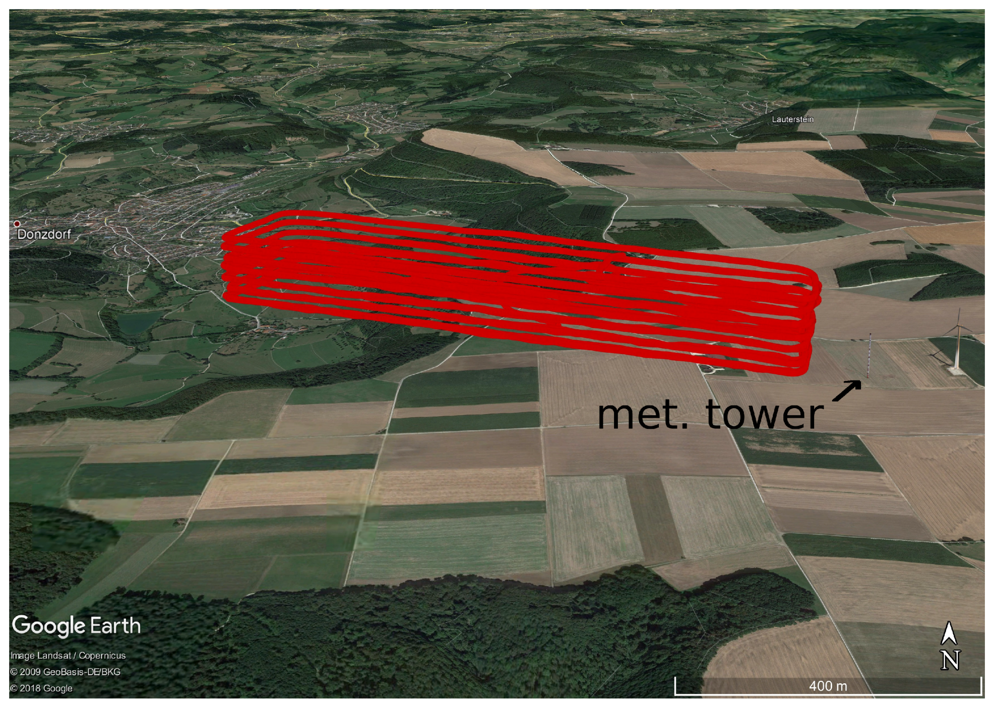
The Schnittlingen (SNT) test site is located in southern Germany on the border of the Swabian Alp. The flight was performed just over the crest, which rises from the valley at about 500 m above mean sea level (AMSL) up to the plateau at 650 m. With westerly wind, the flow was hitting the crest perpendicularly, forming up-drafts and strongly sheared flow in the vicinity. Many flights and other measurement systems, such as LiDAR, have been used to investigate the site. Results from intensive measurements on several days were published by Wildmann et al. [28], and a comparison between sUAV measurements and a numerical simulation of the area was reported by Knaus et al. [49]. For this comparison, a flight on 7 May 2015 was chosen, with overcast and neutral stratification showing the typical phenomena described in these publications. With wind on the ground from the west-northwest direction and an average wind speed of about 6 m s${}^{-1}$, up-drafts over the crest and sheared flow were pronounced. As shown in Figure 7, rectangular so-called racetracks with long legs forth and back over the crest in vertical steps of 25 m were performed. One racetrack comprises two legs including turns or one full round. For every height, two rectangles were flown between 75 and 200 m AGL, summing up to 12 racetracks for the selected data fraction.

A meteorological tower located in the east of the rectangular flight path is available for comparison (Figure 7 and

Table 3. Horizontal wind speed and wind direction at Schnittlingen meteorological tower. Data at 98 m AGL in comparison with the MHPA for the flight on 7 May 2015 between 11:23:16 p.m. and 11:50:46 p.m. local time. Additionally, the data is divided into three intervals of 550 s each.

	11:23:16 a.m. Until 11:50:46 a.m.	First 550 s	Second 550 s	Last 550 s
Tower SNT	$6.02\pm 1.50$ m s${}^{-1}$	$5.28\pm 1.08$ m s${}^{-1}$	$5.47\pm 1.21$ m s${}^{-1}$	$7.30\pm 1.29$ m s${}^{-1}$
	$283\pm {14}^{\circ }$	$282\pm {16}^{\circ }$	$285\pm {13}^{\circ }$	$283\pm {12}^{\circ }$
MHPA SNT	$6.05\pm 1.28$ m s${}^{-1}$	$5.04\pm 0.87$ m s${}^{-1}$	$5.51\pm 0.47$ m s${}^{-1}$	$7.59\pm 0.48$ m s${}^{-1}$
	$286\pm 6^{\circ }$	$286\pm 7^{\circ }$	$290\pm 5^{\circ }$	$281\pm 2^{\circ }$

).

In this complex terrain, the comparison between the meteorological tower and the flight data is not straightforward since surface heterogeneities influence the wind field strongly and the spatial separation between the measurement systems can cause large deviations for the mean flow and the statistics. Nevertheless, the mean values agree very well (Table 3), while the standard deviation in the tower data appears to be larger up to a factor of almost 3 compared to the aircraft data. The higher standard deviation of the tower measurement is caused by the downstream location. As shown by Wildmann et al. [28], the wind field attenuates in this area after the deviation caused by the crest about 1000 m upstream. This causes increased fluctuations and nonstationary behavior. Due to the spatial separation, the data in Table 3 cannot be used for a close comparison, but it shows the development of the wind speed at the site during the experiment. The first period of 550 s represents the four racetracks of the MASC at 75 m and 100 m AGL. During the almost half-hour-long flight, the wind speed varies between approximately 5 m s${}^{-1}$ and 7 m s${}^{-1}$, making the selection interesting when looking at the performance of different wind measurement algorithms.

3.3. Pforzheim (PFR)

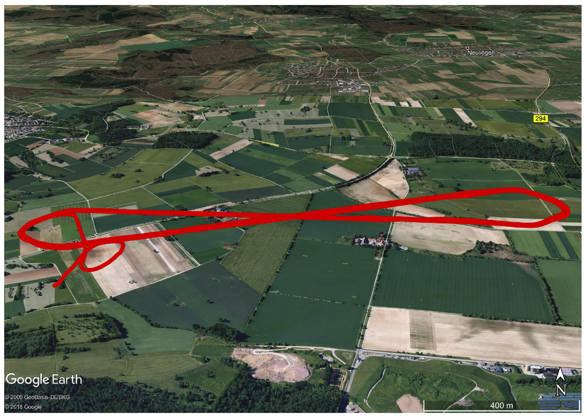
The main reason for this flight was the research of turbulent fluxes in the lower ABL. The test site is located in south Germany close to Pforzheim and near the Rhine rift. The area is flat and extensively used for agriculture. With light winds from the northeast and clear sky conditions, lying eights with long, crossing straights at 150 m AGL (Figure 8) were flown on 11 July in 2013 to investigate the turbulent fluxes above heterogeneous terrain with various agricultural land use. The latent and sensible heat fluxes were significantly large between 9:50:09 a.m. and 10:08:29 a.m. local time, indicating strong convective conditions. The data consists of nine racetracks of about 120 s each.

3.4. Helgoland (HEL)

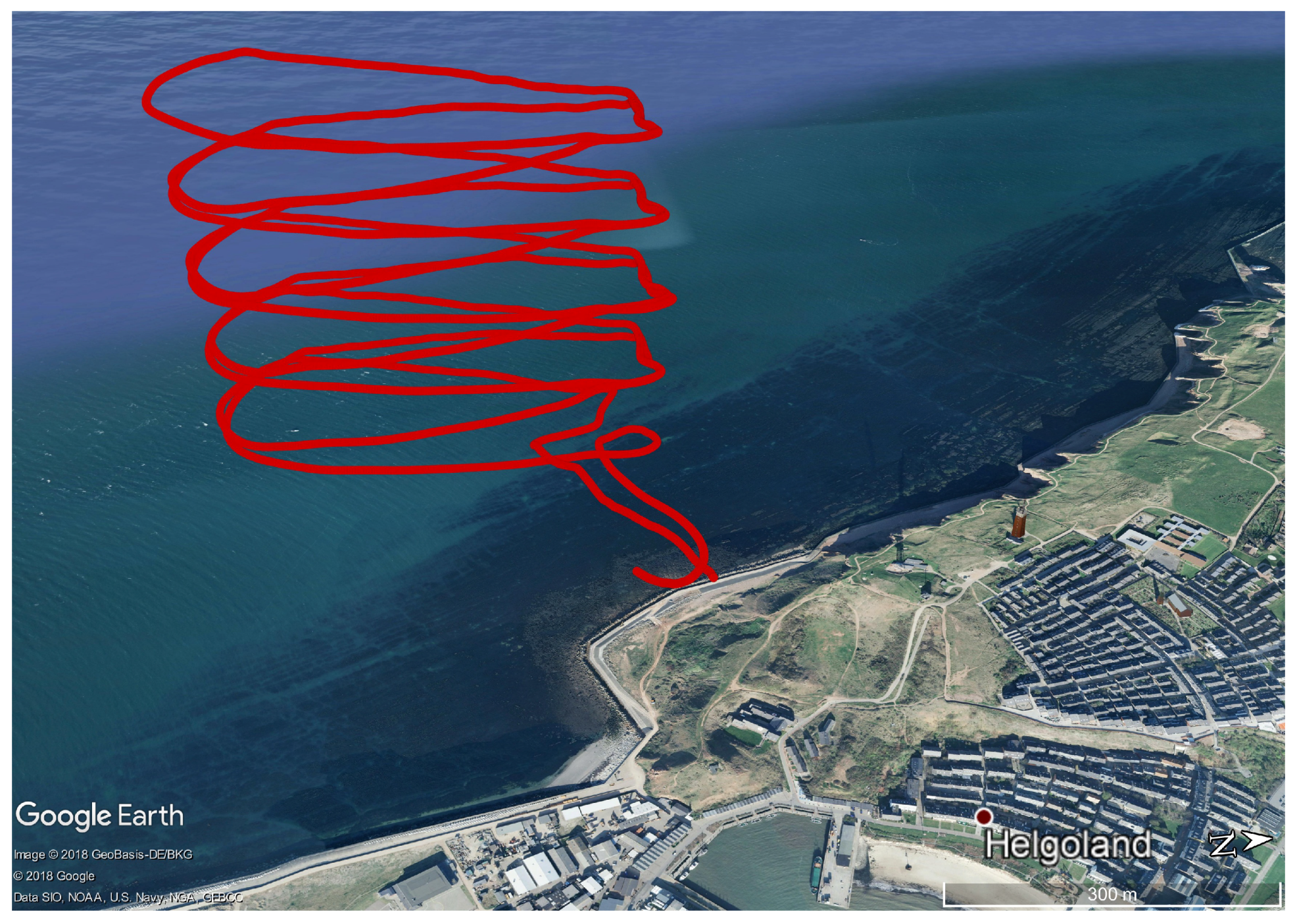
The selected flight from the Helgoland campaign was conducted on 10 October in 2014, during strong wind conditions from the southeast. Helgoland is Germany’s only island in the North Sea with offshore conditions. The undisturbed marine boundary layer with a fetch of several hundred kilometers was measured upstream from the take-off site on the west shore. The data used in this study was gathered during an ascending maneuver from 100 m to 550 m in vertical steps of 50 m. The take-off and landing site, as well as the flight path, are shown in Figure 9. During the long north-south legs, the MASC was climbing 50 m, and the short east-west passages were flown at a constant height. This flight strategy produces data on the vertical profile of various atmospheric quantities. The flight took place between 9:20 a.m. and 9:51 a.m. local time.

4. Results

The set of graphs in the Figure 10, Figure 11, Figure 12 and Figure 13 show scatterplots of the horizontal wind speed and wind direction. Section 2.2.2 and Section 2.2.3 state the importance of the averaging window for the applied simplification of the wind measurement with the NFSA and the PTA. Figure 10 and Figure 11 show the results for an averaging window of $M=240$ s. This timescale comprises at least two full racetracks for all experiments (see Section 3.3). Therefore, this timescale of 4 min is the choice for the comparison and is on the high end of reasonable averaging windows, pledging a robust performance. Longer periods would weaken the studies’ distinctions and not add further comprehension. In comparison, a 1 min averaging time is analyzed, where approximately one racetrack in HEL and two circles at the BAO are inside the averaging window. This is a typical value for averaging in meteorology, where, on the one hand, full racetracks are included and, on the other hand, the performance resulting from data only having fractions of racetracks is addressed. Figure 12 and Figure 13 show these results for an averaging window of $M=60$ s. Preliminary studies showed that significantly shorter periods become unusable for this study since the deviations of the NFSA and the PTA from the MHPA become very large. For quantifying the differences between the algorithms and averaging windows, histograms of the deviation from the MHPA are plotted in Figure 14, Figure 15, Figure 16 and Figure 17. The difference in the horizontal wind speed between the MHPA and the NFSA or the PTA is used. The normalized distribution is presented and the probability density function, together with the fitted normal distribution, is plotted for every experiment and algorithm. The mean $\mu$ of the fitted normal distribution can be interpreted as the bias between the algorithms, and the standard deviation $\sigma$ can be taken as the precision. Each plot contains the results for both averaging periods, $M=240$ s and $M=60$ s, enabling a quantified comparison for each experiment (BAO in Figure 14, SNT in Figure 15, HEL in Figure 16, and PFR in Figure 17) between the averaging windows as well as between the algorithms. It must be noted that the results are also influenced by the tuning of the autopilot and by the aerodynamic design of the sUAS. However, that cannot be analyzed in this study. Furthermore, the airframe and the autopilot for the experiment at the BAO (Skywalker X8 with a Black Swift Technologies LLC autopilot system) and for the other experiments (MASC with the ROCS autopilot) differ and, therefore, the quantified intercomparison between these experiments is influenced by this difference. On the other hand, all experiments were conducted with the same sensor system, and the analysis of the performance of the algorithms when flying different flight patterns is not affected.

4.1. Long Averaging Periods for Robust Performance ($M=240$ s)

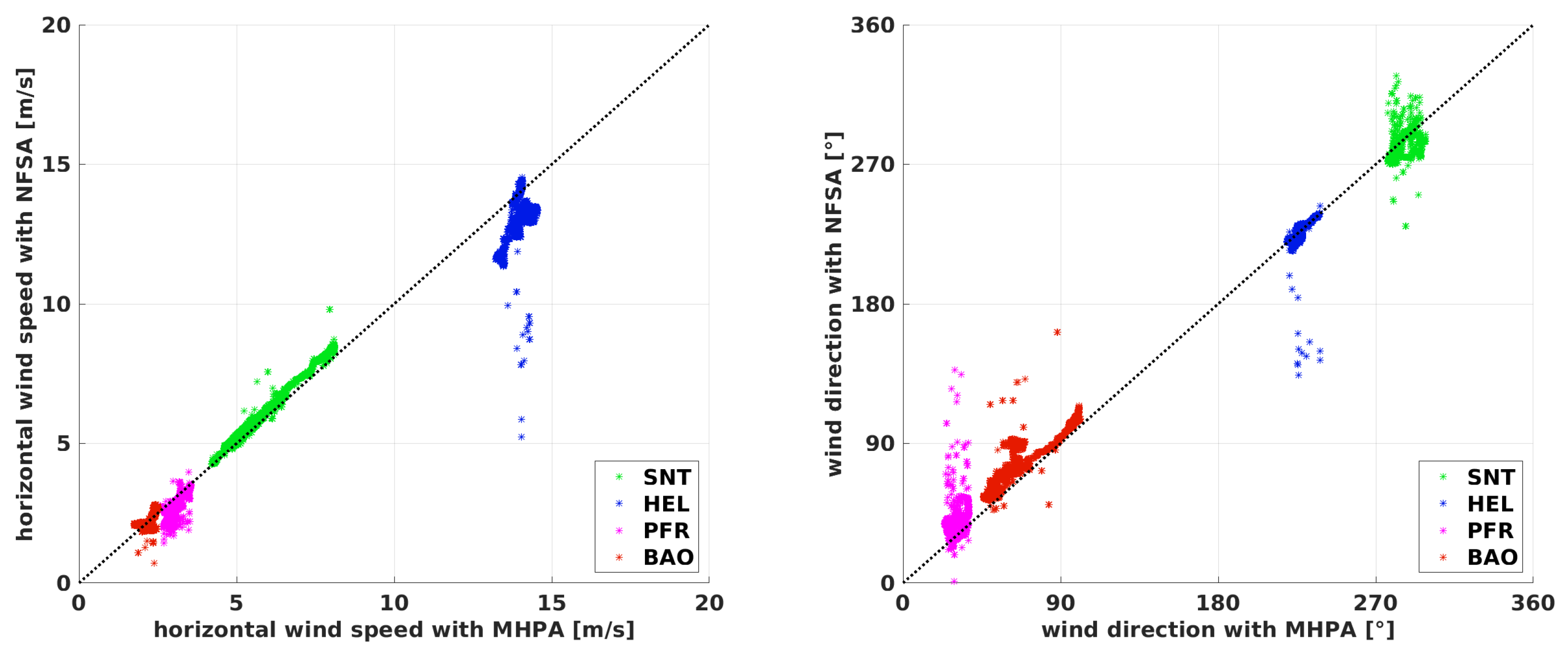
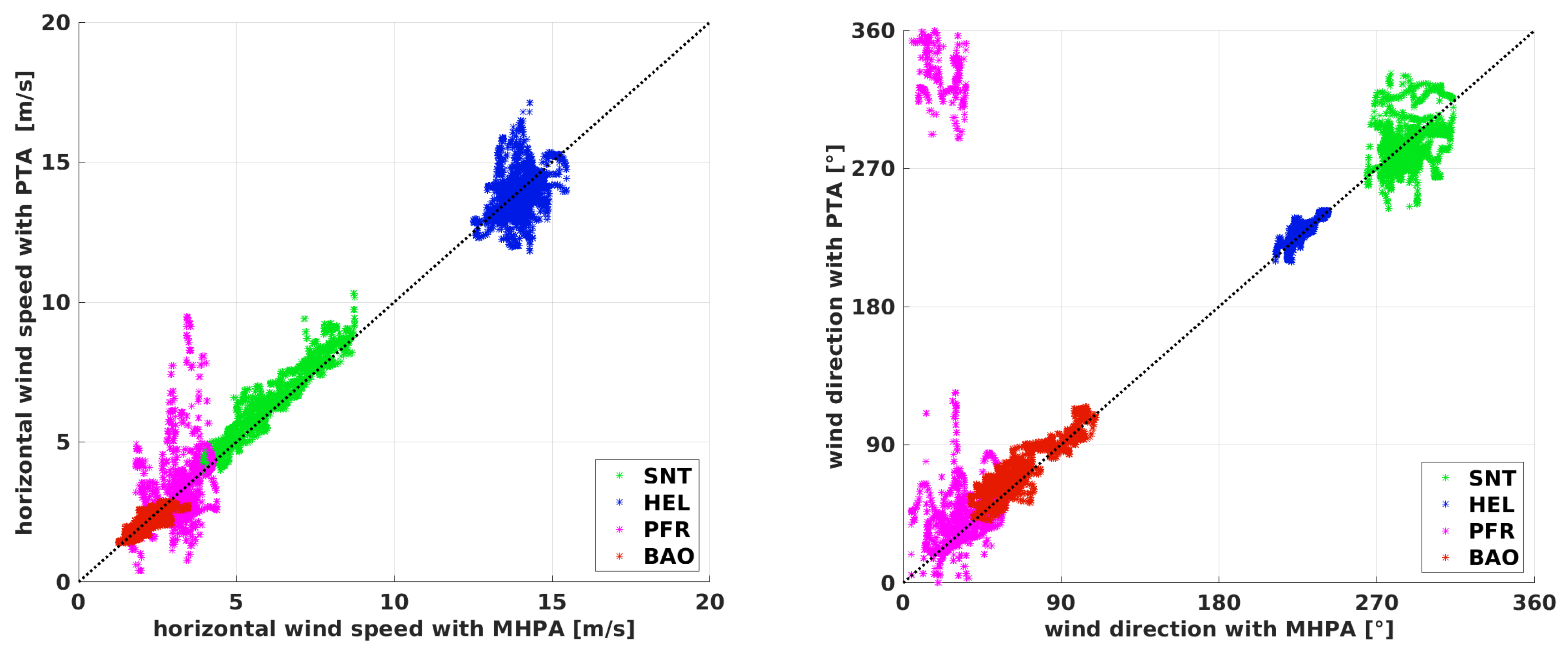
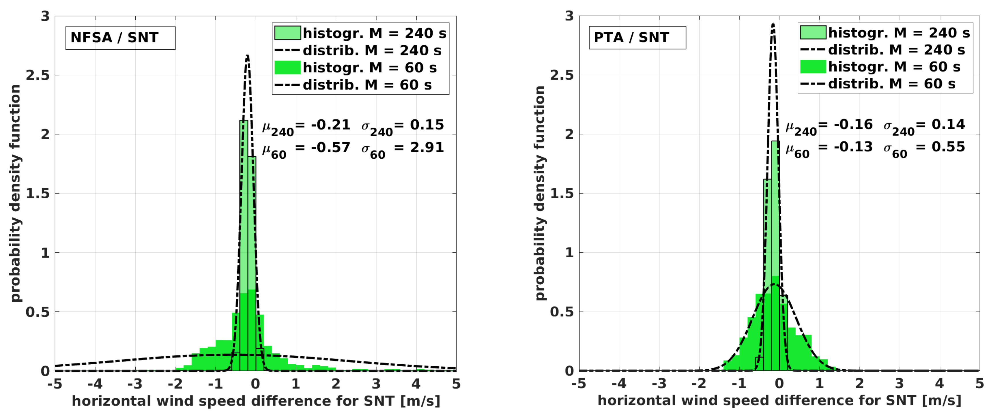
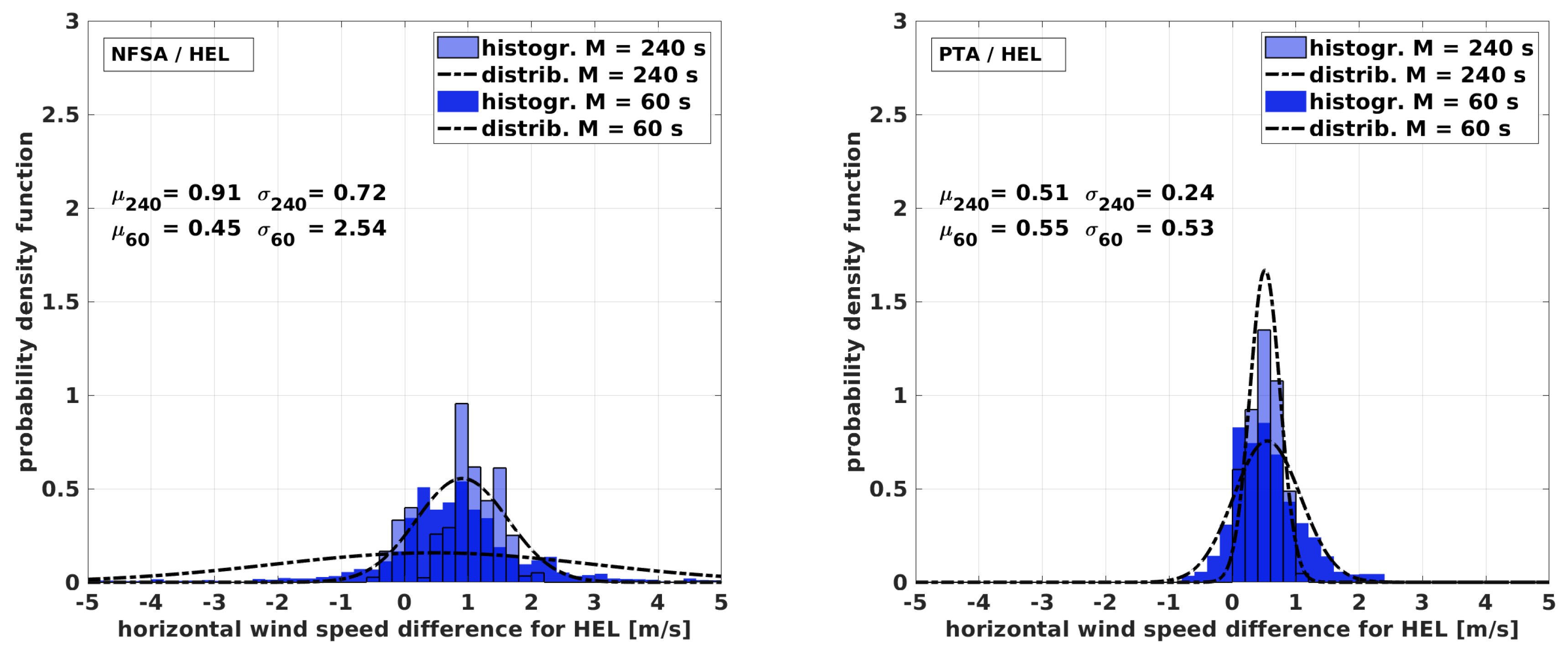
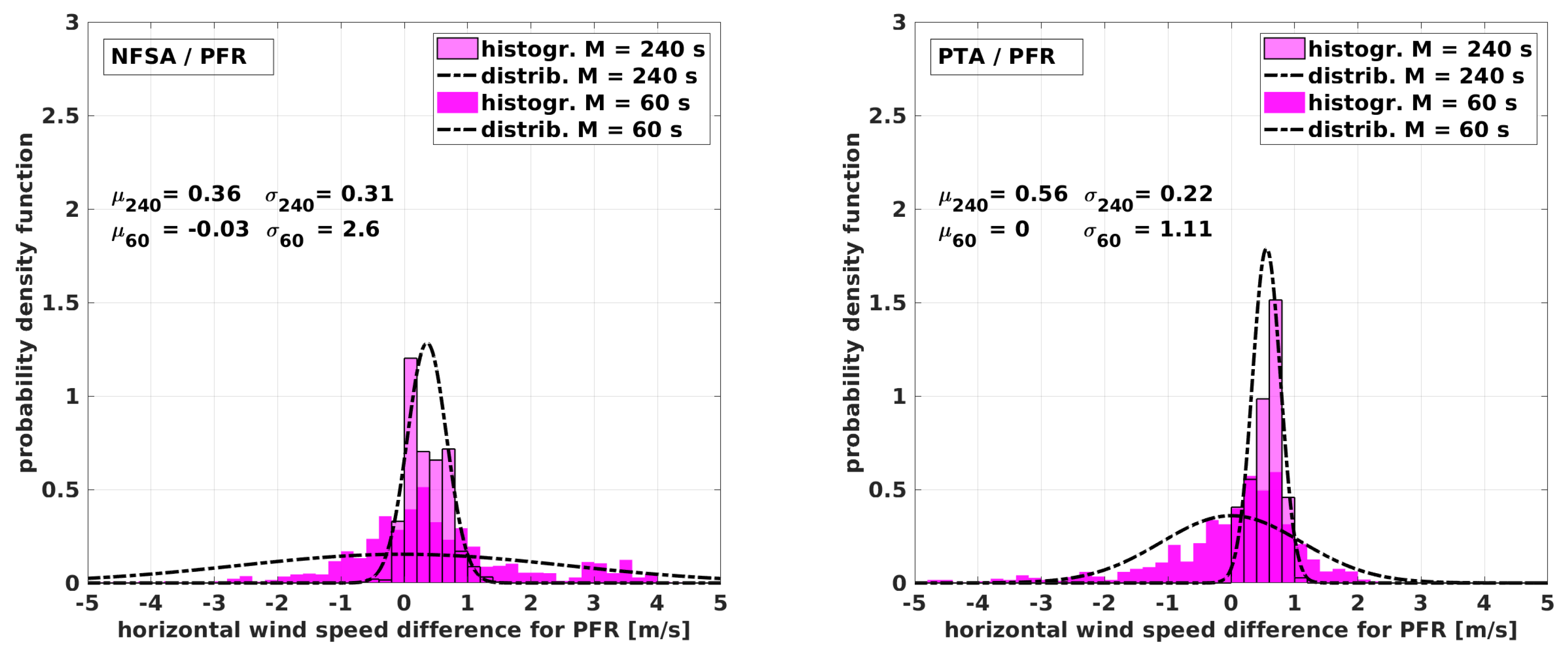
The long period with at least two full racetracks inside the averaging window in Figure 10 and Figure 11 generally shows a good agreement between the different algorithms. Nevertheless, significant differences between the NFSA and the PTA are found. Limitations arise for the NFSA in Figure 10 where large differences for the high wind speeds in HEL occur. The main reason for these is the rapid and inconsistent changes in the heading of the aircraft during the sharp turns caused by the high wind speed and turbulence. This also becomes apparent when looking at Figure 16 where the standard deviation of the fitted normal distribution is the highest for the long averaging period by a factor of 2 ($\sigma =0.72$). Larger differences in the wind speed and especially for the wind direction can also be observed during the very long straights performed in PFR. This is explainable by drifts in the calculated wind speed, which occur because the change rates of the heading during the long straights are too low and the fact that only two racetracks are included. Figure 17 underlines that. The wind direction estimation is generally rather unfavorable with the NFSA. Although long straights lower the confidence, the NFSA is capable of estimating the wind speed and, with reservations, the direction for flight patterns other than circles. The histograms indicate which flight patterns are beneficial when using the NFSA. For two main reasons, the circles at the BAO, but also the horizontal racetracks in SNT, perform best with $M=240$ s. Considerably more than two racetracks comprise the averaging window, and the flight was oriented horizontally. Especially for the experiment in HEL, which has the least favorable conditions for the NFSA, the neglected vertical vector components in Equation (16) become significant. For the HEL experiment, when applying the long averaging period, the NFSA is not capable of estimating the wind speed and direction reliably. On the other hand, for all other experiments, the NFSA yields acceptable results with at least two full racetracks inside the averaging window.

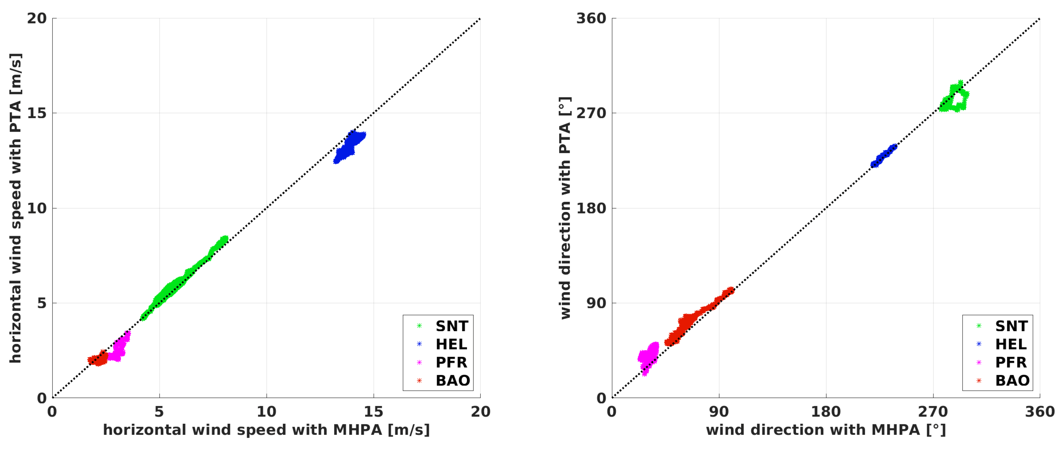
The PTA in Figure 11 shows a very good agreement in its ability to measure the horizontal wind speed precisely in all conditions and for all flight patterns. Taking a closer look at the high wind speeds measured in HEL, the PTA reveals its limitations when used during ascents. The vertical component of the airspeed during ascension results in an underestimation of the horizontal wind speed that is caused directly by the formulation. The same phenomenon is observable during the convective conditions in PFR. The histograms in Figure 16 with a mean of $\mu =0.51$ in HEL and in Figure 17 with a mean of $\mu =0.56$ for the flight in PFR support this and show the limitations for cases with nonzero vertical wind (e.g., flights during convective conditions) or the constant ascent or descent of the sUAS. The effect can be also seen in the NFSA results. For example, this is explainable for the PTA with Equation (8) and the NFSA with Equation (15), where the vertical wind causes an underestimation of the airspeed $\overrightarrow{u_q}$ of the PTA, or of the horizontal airspeed ${\overrightarrow{u}}_g^{(h)}$ of the NFSA. This error propagates through the algorithms and causes an underestimation of the horizontal wind speed. The wind direction estimation with the PTA is robust and reliable in a range of ≈$\pm {10}^{\circ }$, and the wind speed estimation is very good for the long averaging period, with some differences for the strong prevailing vertical motion of either the wind field or the sUAS. Generally, the histograms in Figure 14, Figure 15, Figure 16 and Figure 17 show that the PTA is more precise than the NFSA throughout all the comparisons. Even for the circular flight pattern at the BAO, the PTA performs significantly better since the standard deviation is lower.

4.2. Short Averaging Periods for Enhanced Temporal Resolution ($M=60$ s)

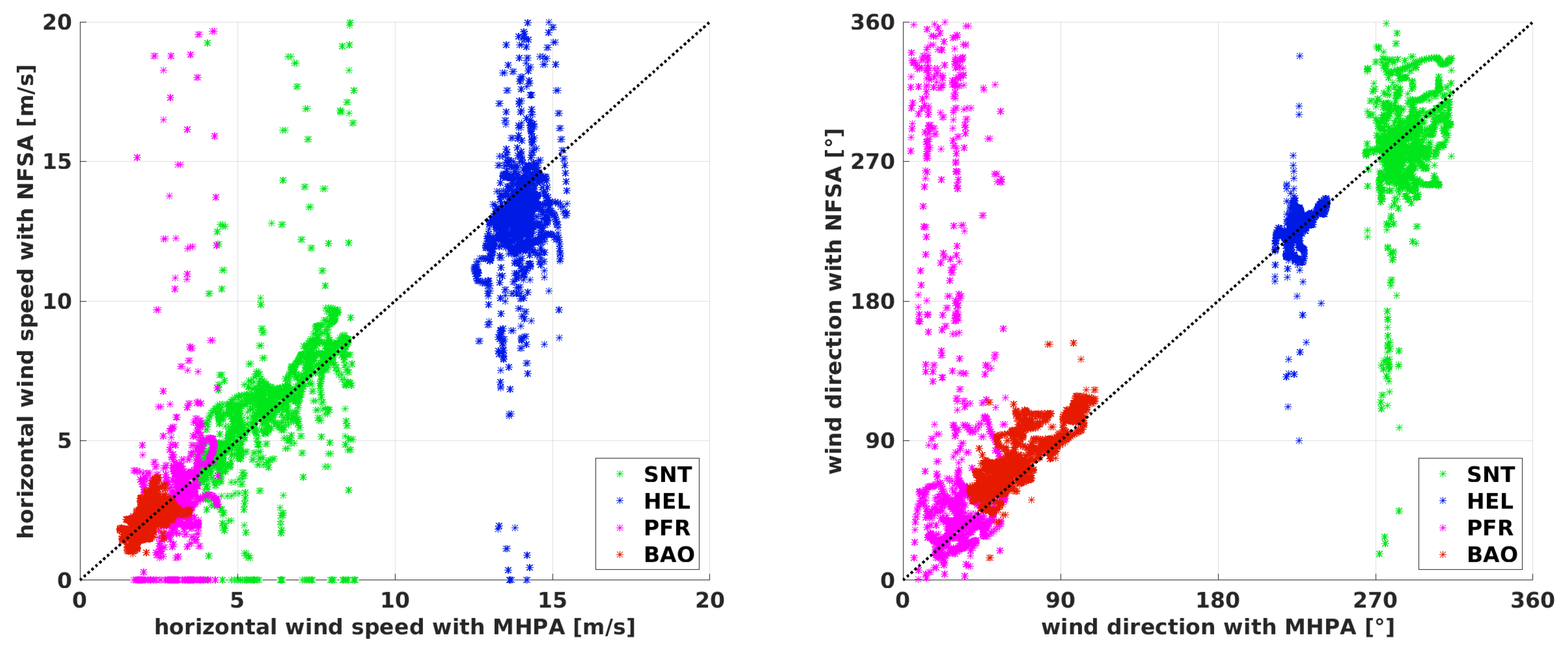
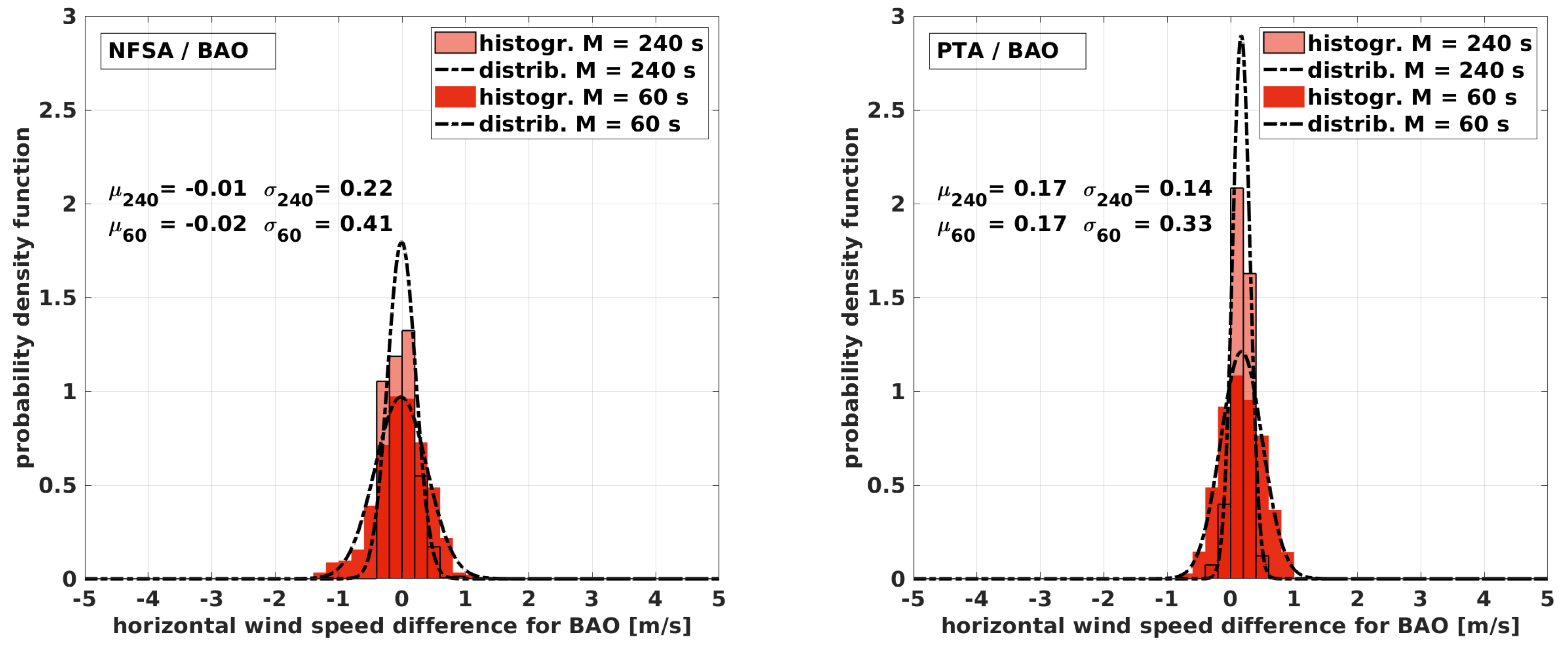
Since 4 min is quite a long averaging time, a 1 min window is presented in Figure 12 and Figure 13 to argue which limitations arise when increasing the temporal resolution. A flight time of 1 min corresponds to only about one leg (half a racetrack) in PFR and in SNT, almost one racetrack in HEL, and two circles or full racetracks at the BAO. To begin with the NFSA in Figure 12, it is evident that the results are quite bad since the scatter is high for a significant portion of the values and for all maneuvers which are not circular. For the BAO flight, the scatter is also significantly higher than for the big averaging window, especially for the wind direction. The standard deviation of the fitted normal distribution in Figure 14 increases from $\sigma =0.22$ to $\sigma =0.41$. This significant decrease in precision appears although there are still two full circles in the averaging window. An explanation is that changes in wind speed and direction at scales smaller than a circle are inadequately represented by the algorithm. These small structures in the wind field cause the aircraft to bear away, leading to a false emphasis on the calculation of mean values when averaging too short a period. In other words, if strong and sudden turbulence causes the autopilot to steer the sUAS with a rather strong movement, this section of the flight path is not representative for the mean flow. This is also critical when taking into account that the boundary layer during the experiment at the BAO was relatively calm, and it suggests that the two circles inside the averaging window could perform even worse under more turbulent conditions. The window M can be decreased from 240 s in some conditions but only when having several full racetracks in the averaging window. For the data at the BAO with $M=60$ s, the result varies within a range of ≈2 m s${}^{-1}$ around the MHPA. For the generally low wind speeds during this measurement, this is already a quite large difference, leading to the conclusion that two full circles are not enough for reliable results.

The PTA in Figure 13 shows good agreement, although the scatter of the MHPA data is greater compared to the long averaging period. The standard deviations $\sigma$ of the histograms in Figure 14, Figure 15 and Figure 16 for the BAO, SNT, and HEL experiment increase from $M=240$ s to $M=60$ s by a factor of 2–4, and the deviation stays within a range of ≈2 m s${}^{-1}$ and ≈20${}^{\circ }$. Challenges become visible for the long straights in PFR. The convection is not the biggest contribution to the increased scatter anymore; instead, the fact that the flow information cannot compensate for excessively low change rates in the heading along the averaging window leads to the differences. The solution of the overdetermined matrix in Equation (14) cannot compensate for the occurrence of small-scale fluctuations if the ground speed and heading become almost constant inside the averaging window M. The results for the SNT flight over complex terrain are, on the other hand, remarkably good for these harsh conditions. Here, the benefit of the algorithm compared to the NFSA is shown for situations when there is less than a full racetrack inside the averaging window and, therefore, a quite high temporal resolution. The mean of the fitted normal distribution in Figure 16 for the HEL flight is $\mu =0.55$, which is in the same range as that for the long averaging period. Except for the underestimation of the wind speed described in Section 4.1, the PTA performs well in this strong and turbulent wind field. Even in high wind speeds, turbulence, shear, and strong up-drafts, the PTA is capable of giving a good estimation of wind speed and direction with reasonable resolution. In comparison to the NFSA, the PTA has considerable benefits when using the additional flow information. The limitations are the resolution of the small scales and turbulent features, which only the MHPA can resolve.

4.3. Intercomparison of the Algorithms and Quantification of the Results

The histograms in Figure 14, Figure 15, Figure 16 and Figure 17 show the quantified differences between the algorithms and highlight the advantages of the PTA over the NFSA, as well as the influence of the averaging period on the performance of both algorithms. The intercomparison of the histograms of the four flight experiments also reveals the limitations. The NFSA must comprise at least two full racetracks, and the PTA can cope with fractions of one racetrack as long as there are not exclusively straight flight paths available. The wind speed estimation is better for all experiments and for all averaging periods with the PTA than with the NFSA, as expected. However, the capabilities of the NFSA are surprisingly good not only for circular flight pattern, as long as the averaging window is long enough. For example, this can be seen when looking at the normal distribution with $M=240$ s for the SNT experiment, which is good for both algorithms. The mean of $\mu =-0.21$ for the NFSA is only slightly worse than the $\mu =-0.16$ for the PTA, with the standard deviations being the same. On the other hand, it is also evident that the temporal resolution of the NFSA is very limited, since the results are not usable for $M=60$ s in SNT and in general, except for the circular flight at the BAO.

Summarizing the results for the long averaging period of $M=240$ s, the following was found:

• The NFSA is capable of estimating the wind speed, and not only for a circular flight pattern, if at least two full racetracks are inside the averaging window. Limitations arise for non-horizontal flight paths and high turbulence.
• The wind direction estimation is subject to large uncertainties with the NFSA.
• The PTA shows a very good agreement with the MHPA and is capable of measuring the horizontal wind speed and direction in all conditions with good accuracy.
• Fast ascent or descent of the sUAS or strong vertical wind components leads to an underestimation of the horizontal wind speed when using the PTA.

For the short averaging period of $M=60$ s, the following was found:

• The NFSA performs better when more than two racetracks are inside the averaging window, as well as for circular flight pattern. This reveals the very limited resolution.
• The PTA still performs well when only fractions of a racetrack are included in the algorithm. Limits arise when exclusively straight flight sections remain inside the averaging window.
• The PTA is capable of estimating reliably the mean wind speed and direction with a reasonable resolution.

A summary of the intercomparison between the two estimation algorithms for mean wind speed and direction is:

• The PTA is more accurate than the NFSA throughout all comparisons, even for the circular flight pattern.
• The PTA needs an additional sensor to estimate the true airspeed, but it achieves significantly higher accuracy and temporal resolution.

5. Conclusions

This study shows the capabilities and limitations of the commonly used methods for wind vector estimation. The no-flow-sensor algorithm and the more sophisticated pitot tube algorithm are compared with the direct measurement using the multi-hole-probe algorithm on a small UAV. The sensor system used in this work is capable of applying all three methods by neglecting parameters during post-processing. By choosing a variety of flight patterns which are used for meteorological sampling and substantially different weather conditions, the comparison covers a broad band of scenarios. The NFSA is generally not limited to circular patterns, but it performs best when having a continuous and rather constant change in the heading of the aircraft. In these cases, the temporal resolution can be increased, and an averaging window which comprises two full racetracks still generates good results, but the increased temporal resolution comes with lower precision. It is shown that strong turbulence decreases the accuracy. Autopilot systems well tuned to perform regular circles at constant airspeed are crucial for the NFSA. The method is limited in cases with long straights. Using one more piece of information, namely, the vector component of the true airspeed in the flight direction, the wind speed and direction estimation can be strongly enhanced. The PTA allows for generally better results than the NFSA and, in particular, provides additional benefit during flight patterns with long straight legs. Furthermore, the temporal resolution is much better without the need for a full racetrack inside the averaging window, although at least some change in the heading is still needed. Another influencing factor is a nonzero vertical vector component, as seen during ascents in Helgoland and in convective conditions in Pforzheim. The horizontal wind speed is slightly underestimated for these conditions. In conclusion, both estimation algorithms achieve good results when applied within their limitations. The simplicity of the NFSA is attractive for very small platforms, and the sUAS can be designed to be cheap, efficient, and robust enough to withstand miscellaneous environmental conditions. The PTA depends on the dynamic pressure measurement, which adds complexity to the sUAV. However, the enhancement of the wind speed and direction estimation is significant. The MHPA is the most sophisticated method and needs a set of differential pressure sensors in combination with extensive calibration. It is deduced that, of the presented algorithms, the temporal resolution to measure at turbulent scales and the ability to measure the vertical wind component can only be achieved using the MHPA.

References

- Holland, G.; Webster, P.; Curry, J.; Tyrell, G.; Gauntlett, D.; Brett, G.; Becker, J.; Hoag, R.; Vaglienti, W. The Aerosonde robotic aircraft: A new paradigm for environmental observations. Bull. Am. Meteorol. Soc. 2001, 82, 889–901. [Google Scholar] [CrossRef]
- Chilson, P.B.; Bonin, T.A.; Zielke, B.S.; Kirkwood, S. The Small Multi-Function Autonomous Research and Teaching Sonde (Smartsonde): Relating In-Situ Measurements of Atmospheric Parameters to Radar Returns. In Proceedings of the 20th Symposium on European Rocket and Balloon Programmes and Related Research, Hyères, France, 22–26 May 2011; Volume 700, pp. 387–394. [Google Scholar]
- Reuder, J.; Jonassen, M.O. First results of turbulence measurements in a wind park with the Small Unmanned Meteorological Observer SUMO. Energy Procedia 2012, 24, 176–185. [Google Scholar] [CrossRef] [Green Version]
- Altstädter, B.; Platis, A.; Wehner, B.; Scholtz, A.; Wildmann, N.; Hermann, M.; Käthner, R.; Baars, H.; Bange, J.; Lampert, A. ALADINA—An unmanned research aircraft for observing vertical and horizontal distributions of ultrafine particles within the atmospheric boundary layer. Atmos. Meas. Tech. 2015, 8, 1627–1639. [Google Scholar] [CrossRef]
- Kräuchi, A.; Philipona, R. Return glider radiosonde for in situ upper-air research measurements. Atmos. Meas. Tech. 2016, 9, 2535–2544. [Google Scholar] [CrossRef] [Green Version]
- Witte, B.M.; Singler, R.F.; Bailey, S.C. Development of an Unmanned Aerial Vehicle for the Measurement of Turbulence in the Atmospheric Boundary Layer. Atmosphere 2017, 8, 195. [Google Scholar] [CrossRef]
- Kral, S.T.; Reuder, J.; Vihma, T.; Suomi, I.; O’Connor, E.; Kouznetsov, R.; Wrenger, B.; Rautenberg, A.; Urbancic, G.; Jonassen, M.O.; et al. Innovative Strategies for Observations in the Arctic Atmospheric Boundary Layer (ISOBAR)—The Hailuoto 2017 Campaign. Atmosphere 2018, 9, 268. [Google Scholar] [CrossRef]
- Jacob, J.D.; Chilson, P.B.; Houston, A.L.; Smith, S.W. Considerations for Atmospheric Measurements with Small Unmanned Aircraft Systems. Atmosphere 2018, 9, 252. [Google Scholar] [CrossRef]
- Hill, M.; Konrad, T.; Meyer, J.; Rowland, J. A small, radio-controlled aircraft as a platform for meteorological sensors. APL Tech. Dig. 1970, 10, 11–19. [Google Scholar]
- Caltabiano, D.; Muscato, G.; Orlando, A.; Federico, C.; Giudice, G.; Guerrieri, S. Architecture of a UAV for volcanic gas sampling. In Proceedings of the 10th IEEE Conference on Emerging Technologies and Factory Automation (ETFA 2005), Catania, Italy, 19–22 September 2005; Volume 1, p. 6. [Google Scholar]
- Diaz, J.A.; Pieri, D.; Wright, K.; Sorensen, P.; Kline-Shoder, R.; Arkin, C.R.; Fladeland, M.; Bland, G.; Buongiorno, M.F.; Ramirez, C.; et al. Unmanned aerial mass spectrometer systems for in-situ volcanic plume analysis. J. Am. Soc. Mass Spectrom. 2015, 26, 292–304. [Google Scholar] [CrossRef] [PubMed]
- Platis, A.; Altstädter, B.; Wehner, B.; Wildmann, N.; Lampert, A.; Hermann, M.; Birmili, W.; Bange, J. An Observational Case Study on the Influence of Atmospheric Boundary-Layer Dynamics on New Particle Formation. Bound.-Layer Meteorol. 2016, 158, 67–92. [Google Scholar] [CrossRef]
- Schuyler, T.J.; Guzman, M.I. Unmanned Aerial Systems for Monitoring Trace Tropospheric Gases. Atmosphere 2017, 8, 206. [Google Scholar] [CrossRef]
- Hobbs, S.; Dyer, D.; Courault, D.; Olioso, A.; Lagouarde, J.P.; Kerr, Y.; Mcaneney, J.; Bonnefond, J. Surface layer profiles of air temperature and humidity measured from unmanned aircraft. Agron. Sustain. Dev. 2002, 22, 635–640. [Google Scholar] [CrossRef] [Green Version]
- Van den Kroonenberg, A.; Bange, J. Turbulent flux calculation in the polar stable boundary layer: Multiresolution flux decomposition and wavelet analysis. J. Geophys. Res. (Atmos.) 2007, 112. [Google Scholar] [CrossRef] [Green Version]
- Thomas, R.; Lehmann, K.; Nguyen, H.; Jackson, D.; Wolfe, D.; Ramanathan, V. Measurement of turbulent water vapor fluxes using a lightweight unmanned aerial vehicle system. Atmos. Meas. Tech. 2012, 5, 243–257. [Google Scholar] [CrossRef] [Green Version]
- Van den Kroonenberg, A.; Martin, S.; Beyrich, F.; Bange, J. Spatially-averaged temperature structure parameter over a heterogeneous surface measured by an unmanned aerial vehicle. Bound.-Layer Meteorol. 2012, 142, 55–77. [Google Scholar] [CrossRef]
- Beyrich, F.; Bange, J.; Hartogensis, O.K.; Raasch, S.; Braam, M.; van Dinther, D.; Gräf, D.; van Kesteren, B.; Van den Kroonenberg, A.C.; Maronga, B.; et al. Towards a validation of scintillometer measurements: The LITFASS-2009 experiment. Bound.-Layer Meteorol. 2012, 144, 83–112. [Google Scholar] [CrossRef]
- Jonassen, M.O.; Ólafsson, H.; Ágústsson, H.; Rögnvaldsson, Ó.; Reuder, J. Improving high-resolution numerical weather simulations by assimilating data from an unmanned aerial system. Mon. Weather Rev. 2012, 140, 3734–3756. [Google Scholar] [CrossRef]
- Reuder, J.; Ablinger, M.; Agústsson, H.; Brisset, P.; Brynjólfsson, S.; Garhammer, M.; Jóhannesson, T.; Jonassen, M.O.; Kühnel, R.; Lämmlein, S.; et al. FLOHOF 2007: An overview of the mesoscale meteorological field campaign at Hofsjökull, Central Iceland. Meteorol. Atmos. Phys. 2012, 116, 1–13. [Google Scholar] [CrossRef] [Green Version]
- Bonin, T.; Chilson, P.; Zielke, B.; Fedorovich, E. Observations of the early evening boundary-layer transition using a small unmanned aerial system. Bound.-Layer Meteorol. 2013, 146, 119–132. [Google Scholar] [CrossRef]
- Martin, S.; Beyrich, F.; Bange, J. Observing Entrainment Processes Using a Small Unmanned Aerial Vehicle: A Feasibility Study. Bound.-Layer Meteorol. 2014, 150, 449–467. [Google Scholar] [CrossRef]
- Wildmann, N.; Rau, G.A.; Bange, J. Observations of the Early Morning Boundary-Layer Transition with Small Remotely-Piloted Aircraft. Bound.-Layer Meteorol. 2015, 157, 345–373. [Google Scholar] [CrossRef]
- Wainwright, C.E.; Bonin, T.A.; Chilson, P.B.; Gibbs, J.A.; Fedorovich, E.; Palmer, R.D. Methods for evaluating the temperature structure-function parameter using unmanned aerial systems and large-eddy simulation. Bound.-Layer Meteorol. 2015, 155, 189–208. [Google Scholar] [CrossRef]
- Bonin, T.A.; Goines, D.C.; Scott, A.K.; Wainwright, C.E.; Gibbs, J.A.; Chilson, P.B. Measurements of the temperature structure-function parameters with a small unmanned aerial system compared with a sodar. Bound.-Layer Meteorol. 2015, 155, 417–434. [Google Scholar] [CrossRef]
- Båserud, L.; Flügge, M.; Bhandari, A.; Reuder, J. Characterization of the SUMO turbulence measurement system for wind turbine wake assessment. Energy Procedia 2014, 53, 173–183. [Google Scholar] [CrossRef] [Green Version]
- Subramanian, B.; Chokani, N.; Abhari, R.S. Drone-based experimental investigation of three-dimensional flow structure of a multi-megawatt wind turbine in complex terrain. J. Sol. Energy Eng. 2015, 137, 051007. [Google Scholar] [CrossRef]
- Wildmann, N.; Bernard, S.; Bange, J. Measuring the local wind field at an escarpment using small remotely-piloted aircraft. Renew. Energy 2017, 103, 613–619. [Google Scholar] [CrossRef]
- Elston, J.; Argrow, B.; Stachura, M.; Weibel, D.; Lawrence, D.; Pope, D. Overview of Small Fixed-Wing Unmanned Aircraft for Meteorological Sampling. J. Atmos. Ocean. Technol. 2015, 32, 97–115. [Google Scholar] [CrossRef]
- Lenschow, D.H. Probing the Atmospheric Boundary Layer; American Meteorological Society: Boston, MA, USA, 1986; Volume 270. [Google Scholar]
- Van den Kroonenberg, A.; Martin, T.; Buschmann, M.; Bange, J.; Vörsmann, P. Measuring the wind vector using the autonomous mini aerial vehicle M2AV. J. Atmos. Ocean. Technol. 2008, 25, 1969–1982. [Google Scholar] [CrossRef]
- Wildmann, N.; Hofsäß, M.; Weimer, F.; Joos, A.; Bange, J. MASC—A small Remotely Piloted Aircraft (RPA) for wind energy research. Adv. Sci. Res. 2014, 11, 55–61. [Google Scholar] [CrossRef]
- de Jong, R.; Chor, T.; Dias, N. Medição da velocidade do vento a bordo de um Veículo Aéreo Não Tripulado. Ciênc. Nat. 2011, 33, 71–74. [Google Scholar]
- Niedzielski, T.; Skjøth, C.; Werner, M.; Spallek, W.; Witek, M.; Sawiński, T.; Drzeniecka-Osiadacz, A.; Korzystka-Muskała, M.; Muskała, P.; Modzel, P.; et al. Are estimates of wind characteristics based on measurements with Pitot tubes and GNSS receivers mounted on consumer-grade unmanned aerial vehicles applicable in meteorological studies? Environ. Monit. Assess. 2017, 189, 431. [Google Scholar] [CrossRef] [PubMed] [Green Version]
- Mayer, S.; Hattenberger, G.; Brisset, P.; Jonassen, M.; Reuder, J. A ‘no-flow-sensor’ wind estimation algorithm for unmanned aerial systems. Int. J. Micro Air Veh. 2012, 4, 15–30. [Google Scholar] [CrossRef]
- Reuder, J.; Brisset, P.; Jonassen, M.; Müller, M.; Mayer, S. The Small Unmanned Meteorological Observer SUMO: A new tool for atmospheric boundary layer research. Meteorol. Z. 2009, 18, 141–147. [Google Scholar] [CrossRef]
- Mayer, S.; Jonassen, M.O.; Sandvik, A.; Reuder, J. Profiling the Arctic stable boundary layer in Advent valley, Svalbard: measurements and simulations. Bound.-Layer Meteorol. 2012, 143, 507–526. [Google Scholar] [CrossRef]
- Bonin, T.; Chilson, P.; Zielke, B.; Klein, P.; Leeman, J. Comparison and application of wind retrieval algorithms for small unmanned aerial systems. Geosci. Instrum. Methods Data Syst. 2013, 2, 177–187. [Google Scholar] [CrossRef] [Green Version]
- Shuqing, M.; Hongbin, C.; Gai, W.; Yi, P.; Qiang, L. A miniature robotic plane meteorological sounding system. Adv. Atmos. Sci. 2004, 21, 890–896. [Google Scholar] [CrossRef]
- Wildmann, N.; Ravi, S.; Bange, J. Towards higher accuracy and better frequency response with standard multi-hole probes in turbulence measurement with remotely piloted aircraft (RPA). Atmos. Meas. Tech. 2014, 7, 1027–1041. [Google Scholar] [CrossRef] [Green Version]
- Wildmann, N.; Mauz, M.; Bange, J. Two fast temperature sensors for probing of the atmospheric boundary layer using small remotely piloted aircraft (RPA). Atmos. Meas. Tech. 2013, 6, 2101–2113. [Google Scholar] [CrossRef] [Green Version]
- Martin, S.; Bange, J.; Beyrich, F. Meteorological Profiling the Lower Troposphere Using the Research UAV ‘M2AV Carolo’. Atmos. Meas. Tech. 2011, 4, 705–716. [Google Scholar] [CrossRef]
- Boiffier, J.L. The Dynamics of Flight; Wiley: Chichester, UK, 1998; p. 353. [Google Scholar]
- Bange, J. Airborne Measurement of Turbulent Energy Exchange between the Earth Surface and the Atmosphere; Sierke Verlag: Göttingen, Germany, 2009; 174p, ISBN 978-3-86844-221-2. [Google Scholar]
- Lenschow, D. Airplane measurements of planetary boundary layer structure. J. Appl. Meteorol. 1970, 9, 874–884. [Google Scholar] [CrossRef]
- Lenschow, D.; Spyers-Duran, P. Measurement Techniques: Air Motion Sensing; National Center for Atmospheric Research, Bulletin: Boulder, CO, USA, 1989. [Google Scholar]
- Calmer, R.; Roberts, G.C.; Preissler, J.; Sanchez, K.J.; Derrien, S.; O’Dowd, C. Vertical wind velocity measurements using a five-hole probe with remotely piloted aircraft to study aerosol–cloud interactions. Atmos. Meas. Tech. 2018, 11, 2583–2599. [Google Scholar] [CrossRef] [Green Version]
- McKinnon, K.I. Convergence of the Nelder–Mead Simplex Method to a Nonstationary Point. SIAM J. Optim. 1998, 9, 148–158. [Google Scholar] [CrossRef]
- Knaus, H.; Rautenberg, A.; Bange, J. Model comparison of two different non-hydrostatic formulations for the Navier-Stokes equations simulating wind flow in complex terrain. J. Wind Eng. Ind. Aerodyn. 2017, 169, 290–307. [Google Scholar] [CrossRef]
Figure 1.
Research unmanned aerial vehicle (UAV) Multi-purpose Airborne Sensor Carrier (MASC) during take-off with a bungee.
Figure 2.
MASC measurement system with five-hole probe, capacitive humidity sensor and temperature sensor, pressure transducers, inertial navigation system (INS), and the measurement computer AMOC.
Figure 3.
Research UAV Skywalker X8 with the MASC measurement system.
Figure 4.
Top view of the wind measurement with the indices a, b, and g representing, respectively, the aerodynamic, body, and geodetic coordinate systems. is the yaw angle or true heading of the sUAV and is the side slip angle between the aerodynamic and body-fixed coordinate system.
Figure 5.
Vector sum of the no-flow-sensor algorithm (NFSA) with the horizontal ground speed , the horizontal true airspeed , and the horizontal wind speed .
Figure 6.
Flight path in red at the Boulder Atmospheric Observatory (BAO) on 8 August 2014 with the meteorological tower in the northwest. During the measurement, low wind speeds from eastern directions with weak convection prevailed.
Figure 7.
Flight path (so-called racetracks) in red in Schnittlingen (SNT) on 7 May 2015, with the meteorological tower east of the flight path. During the measurement, moderate westerly winds prevailed. The crest forms partial up-drafts and strongly sheared flow.
Figure 8.
Flight path in red near Pforzheim (PFR) on 11 July 2013. During the measurement, low wind speed from northeast directions and pronounced convection prevailed.
Figure 9.
Flight path in red on Helgoland (HEL) on 10 October 2014. The figure shows the flight path on the west coast of Helgoland. The undisturbed marine boundary layer with strong winds from the southeast was measured.
Figure 10.
Comparison of the horizontal wind speed (left) and the wind direction (right) on a window of 4 min for the flights at the Boulder Atmospheric Observatory (BAO), Schnittlingen (SNT), Helgoland (HEL), and Pforzheim (PFR). The black dashed line shows the bisecting line where the multi-hole-probe algorithm (MHPA) equals the no-flow-sensor algorithm (NFSA). The data is calculated on a window with s. The results from the MHPA are plotted against the results from the NFSA.
Figure 11.
Comparison of the horizontal wind speed (left) and the wind direction (right) on a window of 4 min for the flights at the Boulder Atmospheric Observatory (BAO), Schnittlingen (SNT), Helgoland (HEL), and Pforzheim (PFR). The black dashed line shows the bisecting line where the multi-hole-probe algorithm (MHPA) equals the pitot tube algorithm (PTA). The data is calculated on a window with s. The results from the MHPA are plotted against the results from the PTA.
Figure 12.
Comparison of the horizontal wind speed (left) and the wind direction (right) on a window of 1 min for the flights at the Boulder Atmospheric Observatory (BAO), Schnittlingen (SNT), Helgoland (HEL), and Pforzheim (PFR). The black dashed line shows the bisecting line where the multi-hole-probe algorithm (MHPA) equals the no-flow-sensor algorithm (NFSA). The data is calculated on a window with s. The results from the MHPA are plotted against the results from the NFSA.
Figure 13.
Comparison of the horizontal wind speed (left) and the wind direction (right) on a window of 1 min for the flights at the Boulder Atmospheric Observatory (BAO), Schnittlingen (SNT), Helgoland (HEL), and Pforzheim (PFR). The black dashed line shows the bisecting line where the multi-hole-probe algorithm (MHPA) equals the pitot tube algorithm (PTA). The data is calculated on a window with s. The results from the MHPA are plotted against the results from the PTA.
Figure 14.
Normalized distribution and probability density function with the fitted normal distribution for the flight at the Boulder Atmospheric Observatory (BAO). The plots show the deviation between the MHPA and the NFSA (left) and the MHPA and the PTA (right) for s and for s.
Figure 15.
Normalized distribution and probability density function with the fitted normal distribution for the flight over complex terrain near Schnittlingen (SNT). The plots show the deviation between the MHPA and the NFSA (left) and the MHPA and the PTA (right) for s and for s.
Figure 16.
Normalized distribution and probability density function with the fitted normal distribution for the flight in Helgoland (HEL). The plots show the deviation between the MHPA and the NFSA (left) and the MHPA and the PTA (right) for s and for s.
Figure 17.
Normalized distribution and probability density function with the fitted normal distribution for the flight near Pforzheim (PFR). The plots show the deviation between the MHPA and the NFSA (left) and the MHPA and the PTA (right) for s and for s.