Tropical Atlantic Response to Last Millennium Volcanic Forcing


1
Instituto de Geociências, Universidade de Brasília, Campus Universitário Darcy Ribeiro 70910-900 ICC –Ala Central, Brasília, Distrito Federal, Brazil
2
Instituto Oceanográfico, Universidade de São Paulo, Praça do Oceanográfico, 191, Cidade Universitária, 05508-120 São Paulo, Brazil
3
Instituto de Astronomia, Geofísica e Ciências Atmosféricas, Universidade de São Paulo, Rua do Matão, 1226, Cidade Universitária, 05508-090 São Paulo, Brazil
*
Author to whom correspondence should be addressed.
Atmosphere 2018, 9(11), 421; https://doi.org/10.3390/atmos9110421
Submission received: 7 August 2018
/
Revised: 3 October 2018
/
Accepted: 9 October 2018
/
Published: 27 October 2018
(This article belongs to the Special Issue Weather and Climate Extremes: Current Developments)
Abstract
:Climate responses to volcanic eruptions include changes in the distribution of temperature and precipitation such as those associated with El Niño Southern Oscillation (ENSO). Recent studies suggest an ENSO-positive phase after a volcanic eruption. In the Atlantic Basin, a similar mode of variability is referred as the Atlantic Niño, which is related to precipitation variability in West Africa and South America. Both ENSO and Atlantic Niño are characterized in the tropics by conjoined fluctuations in sea surface temperature (SST), zonal winds, and thermocline depth. Here, we examine possible responses of the Tropical Atlantic to last millennium volcanic forcing via SST, zonal winds, and thermocline changes. We used simulation results from the National Center for Atmospheric Research Community Earth System Model Last Millennium Ensemble single-forcing experiment ranging from 850 to 1850 C.E. Our results show an SST cooling in the Tropical Atlantic during the post-eruption year accompanied by differences in the Atlantic Niño associated feedback. However, we found no significant deviations in zonal winds and thermocline depth related to the volcanic forcing in the first 10 years after the eruption. Changes in South America and Africa monsoon precipitation regimes related to the volcanic forcing were detected, as well as in the Intertropical Convergence Zone position and associated precipitation. These precipitation responses derive primarily from Southern and Tropical volcanic eruptions and occur predominantly during the austral summer and autumn of the post-eruption year.
1. Introduction
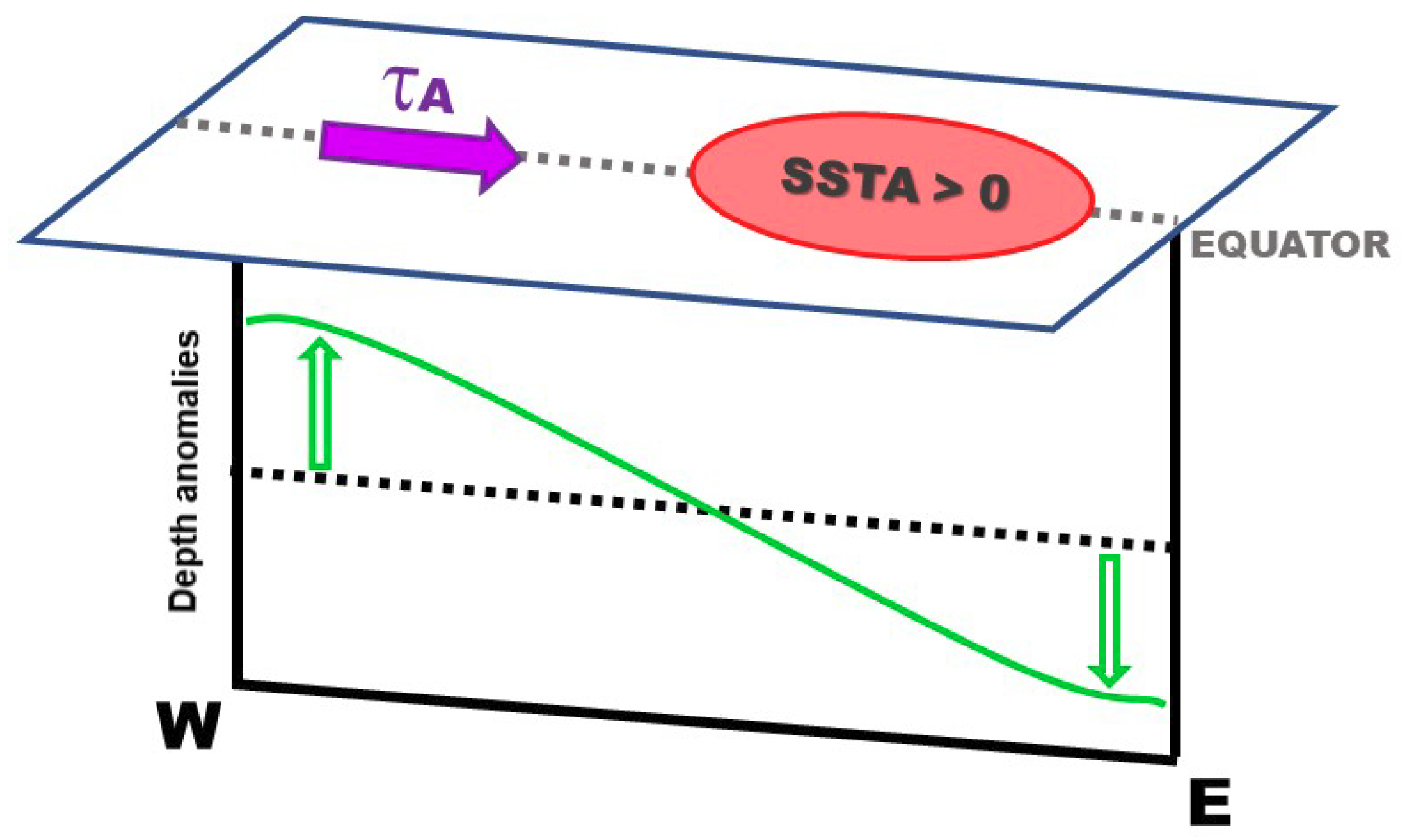
Sea surface temperature (SST) is an important indicator of climate variability. Its response to external forcings will depend on the intensity, duration, and spatial distribution of the perturbation. In the equatorial Atlantic Ocean, noticeable anomalies in SST are observed on interannual time scales. These anomalies reveal the Atlantic Niño mode [1,2], a tongue-shaped SST pattern related to equatorial zonal wind anomalies and thermocline depth changes via air–sea interaction processes. Positive feedback (Figure 1) may occur when the SST and thermocline depth changes in the eastern Atlantic are related to zonal wind anomalies in the western part of the basin [3,4,5]. The Atlantic Niño is known for influencing precipitation in West Africa and South America [6,7,8]. Positive SST anomalies in the eastern equatorial Atlantic increase the precipitation over Northeastern Brazil and western equatorial Amazon, whereas negative SST anomalies in the eastern equatorial Atlantic decrease the precipitation over the West African monsoon region. These patterns correspond to the Atlantic Niño phases and are associated with changes in strength and meridional displacement of the Intertropical Convergence Zone (ITCZ), in intensity of tropical convection, and in magnitude of the westerlies [7,9,10,11,12].
Over the past millennium (850 to 1850 C.E.), strong volcanic eruptions occurred and disturbed the climatic system. Volcanic eruptions may lead to radiative cooling of the surface and troposphere, and to the warming of the stratosphere, by the scattering of visible solar radiation, absorption, and near-infrared, and the absorption and emission of longwave radiation, e.g., reference [2]. This effect is produced by sulfate aerosols resulting from the conversion of sulfur particles emitted by volcanic eruptions that are injected into the stratosphere [12,13]. During the second half of the thirteenth century, many volcanic eruptions promoted a strong cooling of the Earth with long-lasting impacts on the climate [14,15]. The Samalas volcano eruption in 1257 C.E. was the largest one in the last 7000 years and was associated with floods and famine episodes [16]. Ashes and glass from the Samalas eruption were found in both hemispheres as recorded by Greenland and Antarctica ice cores—a typical feature of a volcanic eruption near the equator [13]. Besides 1257 C.E. Samalas event, other great volcanic eruptions occurred during the last millennium such as Kuwae (1452 C.E.), Huaynaputina (1600 C.E.), Laki (1783 C.E.), and Tambora (1815 C.E.) (see [17,18,19] for reconstruction of volcanic eruption events over the past 2500 years). The cooling in 1816 C.E. associated with the Tambora eruption is known for promoting the “year without a summer” in Europe [20]. This extreme climatic condition resulted in the crisis of 1817, with impacts on public health, economy, crop production and starvation Evidence of cooling events as a response to explosive volcanic eruptions was found in tree-ring datasets [21].
Results from numerical model experiments have already shown the impact of volcanic eruptions on the climate system. Some of them include a decrease in temperature and salinity in the Atlantic Ocean [22], changes in the Atlantic Meridional overturning circulation [22,23], a decrease in ocean heat content and sea level [24], a decrease in tropical precipitation [25,26], and changes related to climatic modes of variability such as the El Niño Southern Oscillation (ENSO) [27,28,29,30,31,32]. The large-scale response to volcanic forcing may vary depending on the location of the volcano [31,33] and on the season of the volcanic eruption occurrence [34,35].
An increase in ENSO-positive phase occurrence after the volcanic eruption was identified by some studies [36,37,38], but this response varies among different numerical models [32,35,39,40,41]. The ENSO response to volcanic eruptions is suggested to be a combination of (i) the ocean dynamical thermostat mechanism, in which surface changes are driven by deeper upwelled waters [29] and (ii) air–sea interaction through changes in land–ocean temperature gradient in the Western Pacific [42]. In the Atlantic Niño region, Haywood et al. [43] link 20th century episodes of Sahelian drought to perturbations in the SST influenced by Northern Hemisphere volcanic eruptions. However, they did not investigate possible perturbations of the air–sea interaction processes related to this SST change. Indeed, variations in the equatorial Atlantic upwelling are driven by changes in the thermocline depth and wind-driven equatorial wave effects [44], and perturbation in subsurface temperature [45], but the effects of volcanic eruptions on Tropical Atlantic variability are still poorly understood.
To improve the ability of numerical models to estimate the impacts of external forcings on the climate system, the National Center for Atmospheric Research (NCAR) developed the Community Earth System Model Last Millennium Ensemble (CESM-LME) experiment [46]. The CESM-LME consists of individually natural forced ensembles and full forcing ensembles ranging from the last millennium up to the present (850–2005 C.E.). One of the objectives of CESM-LME is to determine the variability associated with individual natural forcings versus purely internal variability [46]. The Last Millennium (850–1850 C.E.) is the ideal period for the assessment of the relative roles of natural variability and anthropogenic influence, because it corresponds to the most recent time interval with a minor anthropogenic contribution to climate changes. CESM-LME includes a “volcanic-only” ensemble simulation (VOLC) in which volcanism is the only varying natural forcing. Thus, the CESM-LME VOLC is a convenient tool to investigate possible changes in the climate system caused by the volcanic forcing.
Here, we investigate the response of the Tropical Atlantic Ocean to the last millennium volcanic forcing (from 850 to 1850 C.E.) and impacts on South American and West African precipitation using outputs from the CESM-LME experiment. We analyze responses of air–sea interaction variables (SST, zonal winds, and thermocline depth) and the Bjerknes feedback in the Tropical Atlantic under Northern, Southern, and Tropical volcanic eruptions. As previous studies showed that volcanic eruptions disturb SST in Tropical Atlantic, our hypothesis is that volcanic eruptions affect the Bjerknes feedback. Our study is structured as follows: data and methods are described in Section 2, including model details and volcanic forcing. In Section 3, we present results for the volcanism effects of volcanism on the Tropical Atlantic, on Bjerknes feedback indicators, and on African and South American precipitation. In Section 4, we discuss our results and its limitations. Finally, our conclusions are summarized in Section 5.
2. Experiments
2.1. Data and Methods
We used monthly outputs from the CESM-LME [46] (see Section 2.2 for details) of SST, precipitation, wind stress, and temperature fields for the past millennium (850 to 1850 C.E.). Our analysis encompassed outputs in the timespan within 850 to 1850 C.E. (pre-industrial climate) of the VOLC ensemble (five members), and in the “850-control” (CTRL) simulations. We compare the single-forcing ensemble mean simulation (VOLC) with the CTRL scenario. Since we want to investigate only the response to volcanism without other forcings’ influence, as in Zuo et al [47], we opted to use the single-forcing VOLC ensemble members.
To evaluate the Tropical Atlantic variability, we averaged key variables over the eastern Atlantic, ATL3 (20° W–0°; 3° S–3° N) area, as defined by [1], and over the western Atlantic, WATL (40° W–20° W; 3° S–3° N) area, as in [48]. The thermocline depth index (Z20) was considered as the depth of the 20 °C isotherm [49].
A Superposed Epoch Analysis (SEA) was used to isolate the climatic response for the volcanic eruptions, following other studies of volcanism impacts on climate [15,28,36]. For the SEA, we calculated seasonal anomalies with uncertainties represented by twice the standard deviation. We also compared the anomalies with the CTRL standard deviation that corresponds to the natural variability of the climate system. We classified volcanic eruptions according to their location as described in [31] (Table 1). The aerosol mass mixing ratio during the eruption year and two subsequent years were integrated over the Northern and Southern Hemispheres. The resulting ratios between the two were used to classify the eruption: Northern eruption for mixing ratio higher than 1.3, Southern eruption for mixing ratio lower than 0.7, and Tropical eruption for mixing ratio between 0.7 and 1.3 [31]. Only eruptions with a peak mass aerosol mixing ratio greater than 10−8 were used to minimize biases in magnitude of the eruption (more details can be found in [31]).
The Bjerknes feedback was estimated via the relationship between SST, zonal wind stress, and thermocline depth obtained through least squares regressions. We considered regression slopes at 95% confidence levels. Precipitation composites were calculated by averaging precipitation anomalies fields for selected years and using a 95% significance t-test.
2.2. Model Details and Volcanic Forcing
The CESM-LME [46] uses the CESM version 1.1 [50]. Model resolution is ~2° in the atmosphere and the land components, and ~1° in the ocean and sea ice components.
The CESM-LME simulations (more details in [46]) range from 850 to 2005 and consist of different ensembles forced either exclusively with orbital, solar activity, volcanic eruptions, land use, and land change, and greenhouse gases concentrations, or with all forcings concurrently (full-forcing). It follows the Palaeoclimate Modeling Intercomparison Project phase 3 [51] protocols [52,53]. The modulation of insolation by orbital parameters was obtained after Berger [54], and changes in total solar irradiance follow Vieira et al. [55], including the 11-year solar cycle. Greenhouse gases (CO2, CH4, and N2O) concentrations were based on high resolution Antarctica ice cores [52]. Land use and land cover changes derive from a combination of Pongratz et al. [56] and Hurtt et al. [57] datasets. The CTRL experiment ranges from 850 to 2005 and was started from an 1850 control simulation 650-years long [46]. The CTRL is a CESM-LME no-forcing run and therefore employs the same model configurations of the forced runs. However, the CTRL run has preindustrial conditions, with the incoming solar radiation at the top of the atmosphere fixed at 1360.9 W m−2 and CO2 level fixed at 284.7 ppm [58,59].
The volcanic forcing in CESM-LME corresponds to the 54 ice core records compiled by Gao et al. [17]. This dataset contains estimates of stratospheric sulfate aerosol loadings from volcanic eruptions from both the Arctic and Antarctica, modeled as a function of latitude, altitude, and month (volcanic eruptions with unknown seasonality are considered to begin in April). Composite clear-sky albedo for all CESM-LME eruptions are shown in Figure 1 of Stevenson et al. [31].
3. Results
Here, we present results for the Tropical Atlantic response to the last millennium volcanic forcing, via air–sea interaction processes involving changes in SST, zonal wind stress, and thermocline depth, and effects on South America and Africa precipitation.
3.1. Tropical Atlantic During the Last Millennium
The SEA method is applied to seasonal (i) SST variability of the ATL3 index [1], (ii) zonal winds variability in the WATL [3], and (iii) Z20 in the eastern part of the basin [49]. Seasonal analysis corresponds to four periods: December to February (DJF, austral summer), March to May (MAM, austral autumn), June to August (JJA, austral winter), and September to November (SON, austral spring).
The ATL3 SST response to volcanic forcing was different depending on the hemisphere of the volcanic eruption (VOLC, Figure 2) and was detected mainly for the first year after the volcanic eruption (year +1). For NH eruptions, only MAM (Figure 2B) presented a significant cooling (−0.40 ± 0.13 °C) within two standard deviations. A decrease in DJF (0 to +1) SST occurs when considering only one standard deviation. SH volcanic eruptions produced a cooling in DJF (Figure 2E), JJA (Figure 2G), and SON SST (Figure 2H), with the most outstanding cooling during austral spring (−1.20 ± 0.23 °C). TR volcanic eruptions generated cooling during the whole year, with the most prominent SST cooling in SON (Figure 2L) of −1.10 ± 0.45 °C. In all cases, the post-eruption cooling was followed by an increase of the mean SST value in the second or third year after the volcanic eruption. All cases we considered significant were beyond the internal variability, represented by the CTRL standard deviation (0.39 °C, magenta solid line in Figure 2). No significant variability was identified for the CTRL simulation shown in Figure 3.
Examination of both western equatorial Atlantic zonal winds (WATL, VOLC Figure 4, and CTRL Figure 5) and eastern Atlantic thermocline depths (Z20, VOLC Figure 6, and CTRL Figure 7) show no significant response considering two standard deviations of the ensemble mean despite the post-eruption SST cooling identified by the ATL3 SST SEA (Figure 2). Weakening of VOLC zonal wind stress occurs for one standard deviation during MAM, JJA, and SON (Figure 4F,G,H) for SH eruptions, and DJF and MAM (Figure 4I,J) for TR eruptions. A negative deviation of VOLC Z20 occurs for one standard deviation during MAM, JJA, and SON (Figure 6F,G,H) for SH eruptions, and DJF and MAM (Figure 6I,J) for TR eruptions. None of the anomalies rise above the natural variability threshold (CTRL standard deviation; 0.6 10−2 Nm−2 for WATL; 4.3 m for Z20) but the VOLC MAM Z20 (Figure 6J). These results motivated us to examine the air–sea interaction processes related to the Atlantic Niño mode in the VOLC and CTRL experiments (Section 3.2).
3.2. Air–sea Interaction in the Tropical Atlantic
In the Tropical Ocean, three air–sea interaction processes are related to the equatorial modes of variability: (i) eastern SST anomalies forcing western equatorial wind stress anomalies, (ii) western zonal wind stress anomalies forcing thermocline depth anomalies that propagate eastward, and (iii) eastern equatorial SST anomalies induced by local thermocline depths [3,4,5,45,48]. The Bjerknes feedback [60] is characterized when these three elements act simultaneously. In the Tropical Pacific, the Bjerknes feedback drives the ENSO, while in the Tropical Atlantic it is active during the cold tongue season related to the Atlantic Niño [61]. One way to assess the link between SST, zonal winds, and thermocline depth in the Tropical Atlantic is to examine the correlation between them in the air–sea interaction processes cited above [48,62]. The result of the analysis is shown in Figure 8, for both VOLC and CTRL experiments. The calculated regression slopes are displayed in Table 2.
The regression between the ATL3 SST anomalies and the WATL wind stress anomalies (Figure 8A,D) shows a positive relationship (95%-significance) between the variables in both VOLC (0.41 ± 0.01 N m−2 K−1) and CTRL (0.46 ± 0.01 N m−2 K−1) simulations. This relationship was referred to as zonal advection feedback by [4,48], and it is 0.05 ± 0.01 N m−2 K−1 smaller in the VOLC simulation when compared to the CTRL simulation.
The regression between the thermocline slope anomalies, and the WATL wind stress anomalies (Figure 8B,E), represent the thermocline feedback. The thermocline slope anomalies were calculated as the difference between 20°C-isotherm depths anomalies averaged over the ATL3 and WATL regions. The 20°C-isotherm is an indicator of the thermocline depth [49]. A positive regression (95%-significance) was obtained for the thermocline feedback with slope values of 4.28 ± 0.05 m/10−2 N m−2 (VOLC) and 4.02 ± 0.06 m/10−2 N m−2 (CTRL). This air–sea interaction process is 0.26 ± 0.06 m/10-2 N m−2 larger in VOLC when compared to CTRL.
The amplification of the ATL3 SST anomalies by changes in thermocline depths (Figure 8C,F) displayed positive regression (95%-significance) between the referred variables and presented slopes of 2.00 ± 0.05 K m−1 and 2.15 ± 0.06 K m−1 for VOLC and CTRL simulations, respectively. This BF indicator is 0.15 ± 0.06 K m−1 smaller in VOLC when compared to CTRL. The differences detected in the feedback components between VOLC and CTRL are attributed only to the volcanic forcing.
3.3. Effects on Tropical Atlantic
3.3.1. Precipitation
SST changes may directly impact evaporation and precipitation. In the Tropical Atlantic, SST anomalies are related to precipitation changes in both Northeastern Brazil [7,63] and West Africa [6,7]. Thus, we calculated the correlation (95%-significance) between seasonal precipitation and ATL3 SST index for VOLC and CTRL simulations (Figure 9) to access this relationship in the VOLC and CTRL simulations. Results show positive correlation (correlation coefficient R > 0.5) between ATL3 SST and precipitation for VOLC simulation results during austral spring (SON, Figure 9D) in northern South America, eastern equatorial Africa, and over the Tropical Atlantic, and negative correlation (R < −0.5) during austral autumn (MAM, Figure 9B) in northern South America. The difference between VOLC and CTRL simulations (Figure 9I–L) is positive in western Amazon for all seasons, in the Amazon Basin during MAM (Figure 9J), and in equatorial western Africa during JJA (Figure 9K).
Composites of precipitation for volcanic eruptions selected as described in Table 1 were calculated for the first post-eruption year (+1) (Figure 10 for VOLC and Figure 11 for CTRL—only 95% significance t-tested values are shown). Year (+1) is shown solely because we wanted to examine impact of ATL3 SST changes due to volcanic eruptions in precipitation (occurred just in year (+1), as in Figure 2). Results exhibit no statistical significance for NH eruptions in JJA (+1) (Figure 10C) or TR eruptions in SON (+1) (Figure 10L). Dipole-shaped perturbations in precipitation are more prominent over the ocean and in north/northeastern Brazil for NH volcanic eruptions, mainly during MAM (+1) (Figure 10B) and DJF (0 to +1) (Figure 10A). For SH volcanic eruptions, the post-eruption year response is a drier South America and central southern Africa, primarily in DJF (0 to +1) (Figure 10E) and MAM (+1) (Figure 10F). In both JJA (+1) (Figure 10G) and SON (+1) (Figure 10H), the major response is over the Tropical Atlantic. TR volcanic eruptions have had an impact on DJF (0 to +1) (Figure 10I) and MAM (+1) (Figure 6J) precipitation, with drier Amazon region and central southern Africa and wetter eastern Brazil. VOLC simulation (Figure 10) displays a strong response for volcanic eruptions compared to CTRL simulation results (Figure 11).
Impacts of volcanic eruptions on precipitation have been examined by recent studies and may indeed vary depending on the latitudinal location of the volcano. Changes in tropical precipitation were detected in the first post-eruption year during the last millennium [25], whereas the ITCZ shifts away from the hemisphere of the eruption for present climate in Coupled Model Intercomparison Project Phase 5 model outputs [64]. NH eruptions present greater capability of enhancing monsoon-related precipitation in the SH, and so do the SH eruptions in enhancing the monsoon-related precipitation in the NH, mainly via atmospheric circulation changes [26]. Our results suggest that the main impacts of volcanism on precipitation for the South Atlantic area occur for SH eruption and TR volcanoes, with a decrease in precipitation primarily during post-eruption austral summer (DJF 0 to +1) and autumn (MAM +1).
3.3.2. ITCZ shifts
During the first year after NH eruptions (Figure 10A–D), the tropospheric cooling related to the aerosol injection in the stratosphere cools the NH. The SH becomes relatively warmer, leading to enhanced monsoon precipitation in South America during DJF (0 +1) (Figure 10A) and to a southward displacement of the ITCZ during DJF (0 +1), MAM (+1), and SON (+1) (Figure 10A,B,D), which impacts South America during the whole year (+1) but Africa only during SON (+1) (Figure 10D).
For SH eruptions, we observe the opposite scenario (Figure 10E–H). The SH becomes cooler than the NH due to the volcanic aerosols injected into the stratosphere, decreasing the precipitation related to the South American monsoon and to African austral summer in DJF (0 +1) (Figure 10E). However, the ITCZ shifts towards the NH are less evident during MAM (+1) (Figure 10F) in comparison to NH eruptions (Figure 10B), besides a general decrease in precipitation on South America and Africa. The northward displacement of the ITCZ is also observed during JJA (+1) (Figure 10G), but mainly during SON (+1) (Figure 10H).
The TR eruptions effects on precipitation present a less clear spatial pattern (Figure 10I–L). The induced cooling in the tropical region results in less precipitation, mainly during austral summer and autumn. DJF (0 +1) precipitation response to TR eruption (Figure 10I) resembles the pattern observed during the same period but for SH eruptions (Figure 10E) and represents a decrease in South American monsoon precipitation and in austral summer African precipitation. During MAM (+1), there is a decrease in tropical precipitation after TR eruptions (Figure 10J), but the ITCZ shift is not as clear as it was for NH and SH eruptions.
4. Discussion
Model errors and biases are continuously addressed in climate studies as numerical models evolve in temporal and spatial resolution. In the tropical region, representing air–sea interaction processes that involve precipitation, SST, and winds is a difficult task, mainly because of inaccurate, large-scale atmospheric pressure fields; clouds parameterization; and dynamics affecting seasonal SST [65]. Despite the continuous effort to improve models, biases are still present. In the Tropical Atlantic, biases in SST due to unrealistic easterlies intensity have direct impact on thermocline depth and the Bjerknes feedback [45,62,66]. Biases in the precipitation field (e.g., displacement of maxima) may imply a misplacement of the ITCZ and change in ocean conditions [67]. Other biases are related to Tropical Atlantic mean state and variability [68], cloud cover [69], and heat content [45].
Being aware of the climatic processes that are not well represented in models is critical for assessing their ability to describe reality and for evaluating paleoclimate simulations. Investigating past climates is useful to examine the climate system response to different forcings. Nonetheless, the sensitivity of the model to external forcing can result in overestimation or underestimation of its impact. Thus, despite previous studies suggesting an increase in ENSO-positive phase occurrence after a volcanic eruption [28,29,36], an erroneous El Niño-like pattern could be obtained if the model overestimates the strength of the eruptions [31]. Another factor that could lead to misinterpretation of the climate system response to external forcings is the forcing itself, since it is derived from proxy reconstructions.
Besides model errors, climate dynamics are constantly under investigation. In the Tropical Atlantic, Deppenmeier et al. [45] estimated the Bjerknes feedback components for CMIP5 models and obtained deviations in ATL3 SST amplification when compared to reanalysis results. They attribute these disparities to a weaker influence of heat content anomalies on eastern Atlantic SSTs and to a slow adjustment of the subsurface ocean to SST anomalies in the Atlantic Niño area. More recently, Wang et al. [44] used the Zebiak-Cane model to show that the annual upwelling in the equatorial Atlantic is driven by two different mechanisms: the western component is dictated by Ekman pumping, whereas the eastern component is forced by changes in thermocline depth and wind-driven equatorial wave effects, pointing to the complexity of Tropical Atlantic variability.
Using the CESM-LME single-forcing VOLC ensemble, we found that only SST responded to last millennium volcanic forcing in the Tropical Atlantic, while zonal winds and thermocline depth presented no significant response. A cooling of the Tropical Atlantic occurred in the post-eruption year, consistent with previous studies [13,24,70,71]. The volcanic forcing provokes a cooling of the surface that decreases global precipitation, mainly in tropical regions [25,26]. Previous studies have shown different responses of the precipitation field to the volcanic forcing depending on both the location of the volcano [31,34] and the season of the year the eruption occurred [35]. Our results show that tropical eruptions decrease tropical precipitation in the Atlantic sector. Higher latitude eruptions displace the ITCZ towards the warmer hemisphere, i.e., to the hemisphere opposite to the eruption. In the South Atlantic region, this implies an enhanced South American Monsoon one year after NH eruptions and a weakened South American Monsoon one year after SH eruptions. In Africa, however, the response is more evident when the South Atlantic is cooler one year after SH and TR eruptions leading to a decrease in precipitation.
5. Conclusions
In this study, we have investigated the response of the Tropical Atlantic to the last millennium volcanic forcing using tropical air–sea interaction variables derived from the single-forcing outputs of the CESM-LME. Our results show that the tropical SST cooling obtained one year after the eruptions did not impact the zonal wind stress or the thermocline depth, suggesting that volcanic eruptions cause radiative cooling in the Tropical Atlantic with no significant effect on air–sea interaction. Nonetheless, differences in the Bjerknes feedback indicators and changes in South American and African precipitation were obtained. The response depends on the location of the volcano, where the ITCZ moves towards the opposite hemisphere of the eruption, leading to a decrease in precipitation in the hemisphere where the eruption occurred. These effects occurred mainly during the austral summer and autumn of the post-eruption year, and represent changes in the South American Monsoon System precipitation regime.
Author Contributions
L.F.P and I.W designed the study. The manuscript was written by L.F.P. with contributions from I.W. and P.L.S.D. All authors contributed towards improving the final manuscript.
Funding
This study was developed in scope of the PAlaeo-Constraints on Monsoon Evolution and DYnamics (PACMEDY) Project and supported by Fundação de Amparo à Pesquisa do Estado de São Paulo (FAPESP) (grant number 2015/50686-1), Coordenação de Aperfeiçoamento de Pessoal de Nível Superior (CAPES) (grant number 88882.151076/2017-01), and Conselho Nacional de Desenvolvimento Científico e Tecnológico (CNPq) (grants number 301726/2013-2, 405869/2013-4). This study was financed in part by the Coordenação de Aperfeiçoamento de Pessoal de Nível Superior–Brasil (CAPES)–Finance Code 001 (grant number 88882.151076/2017-01).
Acknowledgments
All authors wish to thank the National Center for Atmospheric Research (NCAR) and B. Otto-Bliesner for making the CESM-LME data available. NCAR is funded by the National Science Foundation. Monthly, daily, and 6-hourly outputs are saved and archived on the Earth System Grid (http://www.earthsystemgrid.org) as a single variable time-series.
Conflicts of Interest
The authors declare no conflict of interest.
References
- Zebiak, S.E. Air-sea interaction in the equatorial Atlantic region. J. Clim. 1993, 6, 1567–1586. [Google Scholar] [CrossRef]
- Chang, P.; Yamagata, T.; Schopf, P.; Behera, S.K.; Carton, J.; Kessler, W.S.; Meyers, G.; Qu, T.; Schott, F.; Shetye, S.; et al. Climate fluctuations of tropical coupled systems–The role of ocean dynamics. J. Clim. 2006, 19, 5122–5174. [Google Scholar] [CrossRef]
- Keenlyside, N.S.; Latif, M. Understanding equatorial Atlantic interannual variability. J. Clim. 2007, 20, 131–142. [Google Scholar] [CrossRef]
- Lübbecke, J.F.; McPhaden, M.J. A comparative stability analysis of Atlantic and Pacific Niño modes. J. Clim. 2013, 26, 5965–5980. [Google Scholar] [CrossRef]
- Dippe, T.; Greatbatch, R.J.; Ding, H. On the relationship between Atlantic Niño variability and ocean dynamics. Clim. Dyn. 2018, 51, 597–612. [Google Scholar] [CrossRef]
- Carton, J.A.; Cao, X.; Giese, B.S.; Da Silva, A.M. Decadal and interannual SST variability in the Tropical Atlantic Ocean. J. Phys. Oceanogr. 1996, 26, 1165–1175. [Google Scholar] [CrossRef]
- Ruiz-Barradas, A.; Carton, J.A.; Nigam, S. Structure of interannual-to-decadal climate variability in the Tropical Atlantic sector. J. Clim. 2000, 13, 3285–3297. [Google Scholar] [CrossRef]
- Tokinaga, H.; Xie, S.P. Weakening of the equatorial Atlantic cold tongue over the past six decades. Nat. Geosci. 2011, 4, 222–226. [Google Scholar] [CrossRef]
- Carton, J.A.; Huang, B. Warm events in the Tropical Atlantic. J. Phys. Oceanogr. 1994, 24, 888–903. [Google Scholar] [CrossRef]
- Servain, J.; Wainer, I.; Ayina, H.L.; Roquet, H. The relationship between the simulated climatic variability modes of the Tropical Atlantic. Int. J. Climatol. 2000, 20, 939–953. [Google Scholar] [CrossRef]
- Okumura, Y.; Xie, S.P. Interaction of the Atlantic equatorial cold tongue and the African monsoon. J. Clim. 2004, 17, 3589–3602. [Google Scholar] [CrossRef]
- Stenchikov, G.L.; Kirchner, I.; Robock, A.; Graf, H.F.; Antuna, J.C.; Grainger, R.; Lambert, A.; Thomason, L. Radiative forcing from the 1991 Mount Pinatubo volcanic eruption. J. Geophys. Res. 1998, 10, 13837–13857. [Google Scholar] [CrossRef]
- Zielinski, G.A. Use of paleo-records in determining variability within the volcanism-climate system. Quat. Sci. Rev. 2000, 19, 417–438. [Google Scholar] [CrossRef]
- Miller, G.H.; Geirsdóttir, A.; Zhong, Y.; Larsen, D.J.; Otto-Bliesner, B.L.; Holland, M.M.; Bailey, D.A.; Refsnider, K.A.; Lehman, S.J.; Southon, J.R.; et al. Abrupt onset of the Little Ice Age triggered by volcanism and sustained by sea-ice/ocean feedbacks. Geophys. Res. Lett. 2012, 39, L02708. [Google Scholar] [CrossRef]
- Sigl, M.; Winstrup, M.; McConnell, J.R.; Welten, K.C.; Plunkett, G.; Ludlow, F.; Büntgen, U.; Caffee, M.; Chellman, N.; Dahl-Jensen, D.; et al. Timing and climate forcing of volcanic eruptions for the past 2500 years. Nature 2015, 523, 543–549. [Google Scholar] [CrossRef] [PubMed] [Green Version]
- Lavigne, F.; Degeai, J.P.; Komorowski, J.C.; Guillet, S.; Robert, V.; Lahitte, P.; Oppenheimer, C.; Stoffel, M.; Vidal, C.M.; Surono; et al. Source of the great A.D. 1257 mystery eruption unveiled, Samalas volcano, Rinjani Volcanic Complex, Indonesia. Proc. Natl. Acad. Sci. USA 2013, 110, 16742–16747. [Google Scholar] [CrossRef] [PubMed] [Green Version]
- Gao, C.; Robock, A.; Ammann, C. Volcanic forcing of climate over the last 1500 years: An improved ice core-based index for climate models. J. Geophys. Res. 2008, 113, D23111. [Google Scholar] [CrossRef]
- Crowley, T.J.; Unterman, M.B. Technical details concerning development of a 1200 yr proxy index for global volcanism. Earth Syst. Sci. Data 2013, 5, 187–197. [Google Scholar] [CrossRef] [Green Version]
- Toohey, M.; Sigl, M. Volcanic stratospheric sulfur injections and aerosol optical depth from 500 BCE to 1900 CE. Earth Syst. Sci. Data 2017, 9, 809–831. [Google Scholar] [CrossRef] [Green Version]
- Brönnimann, S.; Kramer, D. Tambora and the “Year Without A Summer” of 1816. A Perspective on Earth and Human Systems Science; Swiss Commission for Atmospheric Chemistry and Physics: Gerlafingen, Switzerland, 2016; p. 48. ISBN 978-3-905835-46-5. [Google Scholar] [CrossRef]
- Anchukaitis, K.J.; Breitenmoser, P.; Briffa, K.R.; Buchwal, A.; Büntgen, U.; Cook, E.R.; D’Arrigo, R.D.; Esper, J.; Evans, M.N.; Frank, D.; et al. Tree rings and volcanic cooling. Nat. Geosci. 2012, 5, 836–837. [Google Scholar] [CrossRef]
- Ding, H.; Carton, J.A.; Chepurin, G.A.; Stenchikov, G.; Robock, A.; Sentman, L.T.; Krasting, J.P. Ocean response to volcanic eruptions in Coupled Model Intercomparison Project 5 simulations. J. Geophys. Res. Oceans 2014, 119, 5622–5637. [Google Scholar] [CrossRef] [Green Version]
- Stenchikov, G.L.; Delworth, T.L.; Ramaswamy, V.; Stouffer, R.J.; Wittenberg, A.; Zeng, F. Volcanic signals in oceans. J. Geophys. Res. 2009, 114, D16104. [Google Scholar] [CrossRef]
- Church, J.A.; White, N.J.; Arblaster, J.M. Significant decadal-scale impact of volcanic eruptions on sea level and ocean heat content. Nature 2005, 438, 74–77. [Google Scholar] [CrossRef] [PubMed]
- Iles, C.E.; Hegerl, G.C.; Schurer, A.P.; Zhang, X. The effect of volcanic eruptions on global precipitation. J. Geophys. Res. Atmos. 2013, 118, 8770–8786. [Google Scholar] [CrossRef] [Green Version]
- Liu, F.; Chai, J.; Wang, B.; Liu, J.; Zhang, X.; Wang, Z. Global monsoon precipitation responses to large volcanic eruptions. Sci. Rep. 2016, 6, 24331. [Google Scholar] [CrossRef] [PubMed] [Green Version]
- Robock, A.; Taylor, K.E.; Stenchikov, G.L.; Liu, Y. GCM evaluation of a mechanism for El Niño triggering by the El Chichón ash cloud. Geophys. Res. Lett. 1995, 22, 2369–2372. [Google Scholar] [CrossRef]
- Mann, M.E.; Cane, M.A.; Zebiak, S.E.; Clement, A. Volcanic and solar forcing of the tropical Pacific over the past 1000 years. J. Clim. 2005, 18, 447–456. [Google Scholar] [CrossRef]
- Emile-Geay, J.; Seager, R.; Cane, M.A.; Cook, E.R.; Haug, G.H. Volcanoes and ENSO over the past millennium. J. Clim. 2008, 21, 3134–3148. [Google Scholar] [CrossRef]
- Christiansen, B. Volcanic eruptions, large-scale modes in the northern hemisphere, and the El Niño-Southern Oscillation. J. Clim. 2008, 21, 910–922. [Google Scholar] [CrossRef]
- Stevenson, S.; Otto-Bliesner, B.; Fasullo, J.; Brady, E. “El Niño Like” hydroclimate responses to last millennium volcanic eruptions. J. Clim. 2016, 29, 2907–2921. [Google Scholar] [CrossRef]
- Predybaylo, E.; Stenchikov, G.L.; Wittenberg, A.T.; Zeng, F. Impacts of a Pinatubo-size volcanic eruption on ENSO. J. Geophys. Res. Atmos. 2017, 122, 925–947. [Google Scholar] [CrossRef] [Green Version]
- Khodri, M.; Izumo, T.; Vialard, J.; Janicot, S.; Cassou, C.; Lengaigne, M.; Mignot, J.; Gastineau, G.; Guilyardi, E.; Lebas, N.; et al. Tropical explosive volcanic eruptions can trigger El Niño by cooling tropical Africa. Nat. Commun. 2017, 8, 778. [Google Scholar] [CrossRef] [PubMed]
- Colose, C.M.; LeGrande, A.N.; Vuille, M. The influence of volcanic eruptions on the climate of tropical South America during the last millennium in an isotope-enabled general circulation model. Clim. Past 2016, 12, 961–979. [Google Scholar] [CrossRef] [Green Version]
- Stevenson, S.; Fasullo, J.T.; Otto-Bliesner, B.L.; Tomas, R.A.; Gao, C. Role of eruption season in reconciling model and proxy responses to tropical volcanism. Proc. Natl. Acad. Sci. USA 2017, 114, 1822–1826. [Google Scholar] [CrossRef] [PubMed] [Green Version]
- Adams, J.B.; Mann, M.E.; Ammann, C.M. Proxy evidence for an El Niño-like response to volcanic forcing. Nature 2003, 426, 274–278. [Google Scholar] [CrossRef] [PubMed]
- Li, J.; Xie, S.P.; Cook, E.R.; Morales, M.S.; Christie, D.A.; Johnson, N.C.; Chen, F.; D’Arrigo, R.; Fowler, A.M.; Gou, X.; et al. El Niño modulations over the past seven centuries. Nat. Clim. Chang. 2013, 3, 822–826. [Google Scholar] [CrossRef] [Green Version]
- Wahl, E.R.; Diaz, H.F.; Smerdon, J.E.; Ammann, C.M. Late winter temperature response to large tropical volcanic eruptions in temperate western North America: Relationship to ENSO phases. Glob. Planet. Chang. 2014, 122, 238–250. [Google Scholar] [CrossRef]
- Anchukaitis, K.J.; Buckley, B.M.; Cook, E.R.; Cook, B.I.; D’Arrigo, R.D.; Ammann, C.M. Influence of volcanic eruptions on the climate of the Asian monsoon region. Geophys. Res. Lett. 2010, 37, L22703. [Google Scholar] [CrossRef]
- McGregor, S.; Timmermann, A. The effect of explosive tropical volcanism on ENSO. J. Clim. 2011, 24, 2178–2191. [Google Scholar] [CrossRef]
- Stoffel, M.; Khodri, M.; Corona, C.; Guillet, S.; Poulain, V.; Bekki, S.; Guiot, J.; Luckman, B.H.; Oppenheimer, C.; Lebas, N.; et al. Estimates of volcanic-induced cooling in the Northern Hemisphere over the past 1500. Nat. Geosci. 2015, 8, 784–790. [Google Scholar] [CrossRef]
- Ohba, M.; Shiogama, H.; Yokohata, T.; Watanabe, M. Estimates of volcanic-induced cooling in the Northern Hemisphere over the past 1500. J. Clim. 2013, 26, 784–790. [Google Scholar] [CrossRef]
- Haywood, J.M.; Jones, A.; Bellouin, N.; Stephenson, D. Asymmetric forcing from stratospheric aerosols impacts Sahelian rainfall. Nat. Clim. Chang. 2013, 3, 660–665. [Google Scholar] [CrossRef]
- Wang, L.C.; Jin, F.F.; Wu, C.R.; Hsu, H.H. Dynamics of upwelling annual cycle in the equatorial Atlantic Ocean. Geophys. Res. Lett. 2017, 44, 3737–3743. [Google Scholar] [CrossRef]
- Deppenmeier, A.L.; Haarsma, R.J.; Hazeleger, W. The Bjerknes feedback in the Tropical Atlantic in CMIP5 models. Clim. Dyn. 2016, 47, 2691–2707. [Google Scholar] [CrossRef]
- Otto-Bliesner, B.L.; Brady, E.C.; Fasullo, J.; Jahn, A.; Landrum, L.; Stevenson, S.; Rosenbloom, N.; Mai, A.; Strand, G. Climate variability and change since 850 C.E.: An ensemble approach with the Community Earth System Model (CESM). Bull. Amer. Meteor. Soc. 2016, 97, 735–754. [Google Scholar] [CrossRef]
- Zuo, M.; Man, W.; Zhou, T.; Guo, Z. Different impacts of Northern, Tropical, and Southern volcanic eruptions on the Tropical Pacific SST in the Last Millennium. J. Clim. 2018, 31, 6729–6744. [Google Scholar] [CrossRef]
- Lübbecke, J.F.; McPhaden, M.J. Symmetry of the Atlantic Niño mode. Geophys. Res. Lett. 2017, 44, 965–973. [Google Scholar] [CrossRef] [Green Version]
- Yang, H.; Wang, F. Revisiting the thermocline depth in the equatorial Pacific. J. Clim. 2009, 22, 3856–3863. [Google Scholar] [CrossRef]
- Hurrell, J.; Holland, M.M.; Gent, P.R.; Ghan, S.; Kay, J.E.; Kushner, P.J.; Lamarque, J.F.; Large, W.G.; Lawrence, D.; Lindsay, K.; et al. The community earth system model: A framework for collaborative research. Bull. Amer. Meteor. Soc. 2013, 94, 1339–1360. [Google Scholar] [CrossRef]
- Braconnot, P.; Harrison, S.; Kageyama, M.; Bartlein, P.J.; Masson-Delmotte, V.; Abe-Ouchi, A.; Otto-Bliesner, B.; Zhao, Y. Evaluation of climate models using palaeoclimatic data. Nat. Clim. Chang. 2012, 2, 417–424. [Google Scholar] [CrossRef] [Green Version]
- Schmidt, G.A.; Jungclaus, J.H.; Ammann, C.M.; Bard, E.; Braconnot, P.; Crowley, T.J.; Delaygue, G.; Joos, F.; Krivova, N.A.; Muscheler, R.; et al. Climate forcing reconstructions for use in PMIP simulations of the last millennium (v1.0). Geosci. Model Dev. 2011, 4, 33–45. [Google Scholar] [CrossRef] [Green Version]
- Schmidt, G.A.; Jungclaus, J.H.; Ammann, C.M.; Bard, E.; Braconnot, P.; Crowley, T.J.; Delaygue, G.; Joos, F.; Krivova, N.A.; Muscheler, R.; et al. Climate forcing reconstructions for use in PMIP simulations of the last millennium (v1.1). Geosci. Model Dev. 2012, 5, 185–191. [Google Scholar] [CrossRef] [Green Version]
- Berger, A. Long-term variations of daily insolation and quaternary climatic changes. J. Atmos. Sci. 1978, 35, 2362–2367. [Google Scholar] [CrossRef]
- Vieira, L.E.A.; Solanki, S.K.; Krivova, N.A.; Usoskin, I. Evolution of the solar irradiance during the Holocene. Astron. Astrophys. 2011, 531, A6. [Google Scholar] [CrossRef] [Green Version]
- Pongratz, J.; Reick, C.H.; Raddatz, T.; Claussen, M. A reconstruction of global agricultural areas and land cover for the last millennium. Glob. Biogeochem. Cycles 2008, 22, GB3018. [Google Scholar] [CrossRef]
- Hurtt, G.C.; Chini, L.P.; Frolking, S.; Betts, R.A.; Feddema, J.; Fischer, G.; Fisk, J.P.; Hibbard, K.; Houghton, R.A.; Janetos, A.; et al. Harmonization of land-use scenarios for the period 1500–2100: 600 years of global gridded annual land-use transitions, wood harvest, and resulting secondary lands. Clim. Chang. 2011, 109, 117–161. [Google Scholar] [CrossRef] [Green Version]
- Gent, P.R.; Danabasoglu, G.; Donner, L.J.; Holland, M.M.; Hunke, E.C.; Jayne, S.R.; Lawrence, D.M.; Neale, R.B.; Rasch, P.J.; Vertenstein, M.; et al. The Community Climate System Model version 4. J. Clim. 2011, 24, 4973–4991. [Google Scholar] [CrossRef]
- Landrum, L.; Otto-Bliesner, B.L.; Wahl, E.R.; Conley, A.; Lawrence, P.J.; Rosenbloom, N.; Teng, H. Last millennium climate and its variability in CCSM4. J. Clim. 2013, 26, 1085–1111. [Google Scholar] [CrossRef]
- Bjerknes, J. Atmospheric teleconnections from the equatorial Pacific. Mon. Weather. Rev. 1969, 97, 163–172. [Google Scholar] [CrossRef]
- Richter, I.; Xie, S.P.; Morioka, Y.; Doi, T.; Taguchi, B.; Behera, S. Phase locking of equatorial Atlantic variabililty through the seasonal migration of the ITCZ. Clim. Dyn. 2016, 48, 1–15. [Google Scholar] [CrossRef]
- Richter, I.; Xie, S.P.; Wittenberg, A.T.; Masumoto, Y. Tropical Atlantic biases and their relation to surface wind stress and terrestrial precipitation. Clim. Dyn. 2012, 38, 985–1001. [Google Scholar] [CrossRef]
- Nobre, P.; Shukla, J. Variations of sea surface temperature, wind stress, and rainfall over the Tropical Atlantic and South America. J. Clim. 1996, 9, 2464–2479. [Google Scholar] [CrossRef]
- Iles, C.E.; Hegerl, G.C. The global precipitation response to volcanic eruptions in the CMIP5 models. Environ. Res. Lett. 2014, 9, 104012. [Google Scholar] [CrossRef]
- Grodsky, S.A.; Carton, J.A.; Nigam, S.; Okumura, Y.M. Tropical Atlantic biases in CCSM4. J. Clim. 2012, 25. [Google Scholar] [CrossRef]
- Richter, I.; Xie, S.P. On the origin of equatorial Atlantic biases in coupled general circulation models. Clim. Dyn. 2008, 31, 587–598. [Google Scholar] [CrossRef]
- Siongco, A.C.; Hohenegger, C.; Stevens, B. The Atlantic ITCZ bias in CMIP5 models. Clim. Dyn. 2015, 45, 1169–1180. [Google Scholar] [CrossRef]
- Breugem, W.P.; Hazeleger, W.; Haarsma, R. Multimodel study of Tropical Atlantic variability and change. Geophys. Res. Lett. 2006, 33, L23706. [Google Scholar] [CrossRef]
- Li, G.; Xie, S.P. Origins of tropical-wide SST biases in CMIP multi-model ensembles. Geophys. Res. Lett. 2012, 39, L22703. [Google Scholar] [CrossRef]
- Otterå, O.H.; Bentsen, M.; Drange, H.; Suo, L. External forcing as a metronome for Atlantic multidecadal variability. Nat. Geosci. 2010, 3, 688–694. [Google Scholar] [CrossRef]
- Robock, A. Volcanic eruptions and climate. Rev. Geophys. 2000, 38, 191–219. [Google Scholar] [CrossRef] [Green Version]
Figure 1.
Schematic air–sea interaction in a positive Bjerknes feedback scenario, where the blue horizontal rectangle represents the Tropical Atlantic Basin, and the black vertical rectangle represents a thermocline depth-profile. Positive sea surface temperature anomalies (SSTA, red ellipse) induce zonal wind stress anomalies (τA, violet arrow), and result in thermocline depth anomalies (green line).

Figure 2.
VOLC SEA for ATL3 SST seasonal anomalies (°C), calculated considering the volcanic eruptions listed in Table 1, for five years before the eruption, and ten years after the eruption. Horizontal: class of the eruptions (NH—(A–D); SH—(E–H); and TR—(I–L)); Vertical: seasonal SEA seasonal SEA (December to February—DJF; March to May—MAM; June to August—JJA; and September to November—SON). Lines in colors correspond to the individual ensemble members, and black thick line refers to the ensemble mean. Light shaded gray corresponds to one standard deviation, and dark shaded gray corresponds to two standard deviations. Magenta solid line corresponds to one standard deviation of the CTRL run.

Figure 3.
CTRL SEA for ATL3 SST seasonal anomalies (°C), calculated after list of volcanic eruptions in Table 1, for five years before the eruption and ten years after the eruption. Horizontal: class of the eruptions (NH—(A–D); SH—(E–H); and TR—(I–L)); Vertical: seasonal SEA (December to February—DJF; March to May—MAM; June to August—JJA; and September to November—SON). Dark red line corresponds to the CTRL run, and light shaded red corresponds to one standard deviation of the CTRL run.

Figure 4.
VOLC SEA for WATL wind stress seasonal anomalies (10−2 Nm−2), calculated considering the volcanic eruptions listed in Table 1, for five years before the eruption and ten years after the eruption. Horizontal: class of the eruptions (NH—(A–D); SH—(E–H); and TR—(I–L)); Vertical: seasonal SEA (December to February—DJF; March to May—MAM; June to August—JJA; and September to November—SON). Lines in colors correspond to the individual ensemble members, and black thick line refers to the ensemble mean. Light shaded gray corresponds to one standard deviation, and dark shaded gray corresponds to two standard deviations. Magenta solid line corresponds to one standard deviation of the CTRL run.

Figure 5.
CTRL SEA for WATL wind stress seasonal anomalies (10−2 Nm−2), calculated after list of volcanic eruptions in Table 1, for five years before the eruption and ten years after the eruption. Horizontal: class of the eruptions (NH—(A–D); SH—(E–H); and TR—(I–L)); Vertical: seasonal SEA (December to February—DJF; March to May—MAM; June to August—JJA; and September to November—SON). Dark red line corresponds to the CTRL run, and light shaded red corresponds to one standard deviation of the CTRL run.

Figure 6.
VOLC SEA for thermocline depth seasonal anomalies (m), calculated considering the volcanic eruptions listed in Table 1, for five years before the eruption and ten years after the eruption. Horizontal: class of the eruptions (NH—(A–D); SH—(E–H); and TR—(I–L)); Vertical: seasonal SEA (December to February—DJF; March to May—MAM; June to August—JJA; and September to November—SON). Lines in colors correspond to the individual ensemble members, and black thick line refers to the ensemble mean. Light shaded gray corresponds to one standard deviation, and dark shaded gray corresponds to two standard deviations. Magenta solid line corresponds to one standard deviation of the CTRL run.

Figure 7.
CTRL SEA for Z20 anomalies m), calculated after list of volcanic eruptions in Table 1, for five years before the eruption and ten years after the eruption. Horizontal: class of the eruptions (NH—(A–D); SH—(E–H); and TR—(I–L)); Vertical: seasonal SEA (December to February—DJF; March to May—MAM; June to August—JJA; and September to November—SON). Dark red line corresponds to the CTRL run, and light shaded red corresponds to one standard deviation of the CTRL run.

Figure 8.
Tropical Atlantic air–sea interaction indicators for (A–C) VOLC and (D–F) CTRL simulations, represented by linear regressions of monthly values. First column refers to ATL3 SST and WATL zonal wind stress anomalies, second column refers to equatorial thermocline slope and WATL wind stress anomalies, and third column refers to ATL3 SST and ATL3 thermocline depth anomalies. Thermocline depth is defined as the 20 °C-isotherm depth. Slopes and correlation were both calculated with 95% significance. The calculated regression slopes are also displayed in Table 2.

Figure 9.
Seasonal correlation between precipitation and ATL3 SST index (at 95% significance level). Vertical: seasonal correlation (December to February—DJF; March to May—MAM; June to August—JJA; and September to November—SON). Horizontal: VOLC ensemble mean (A–D), CTRL simulation (E–H), and difference between VOLC and CTRL (I–L). Only statistically significant values are shown.

Figure 10.
VOLC precipitation composites (mm/3 months) for one year after volcanic eruption as listed in Table 1. Lines correspond to the class of the eruptions (NH—(A–D); SH—(E–H); and TR—(I–L)), and columns refer to the seasonal SEA (DJF, MAM, JJA, and SON).
Figure 10.
VOLC precipitation composites (mm/3 months) for one year after volcanic eruption as listed in Table 1. Lines correspond to the class of the eruptions (NH—(A–D); SH—(E–H); and TR—(I–L)), and columns refer to the seasonal SEA (DJF, MAM, JJA, and SON).

Figure 11.
CTRL precipitation composites for one year after volcanic eruption years as listed in Table 1. Lines correspond to the class of the eruptions NH—(A–D); SH—(E–H); and TR—(I–L), and columns refer to the seasonal SEA (DJF, MAM, JJA, and SON).
Figure 11.
CTRL precipitation composites for one year after volcanic eruption years as listed in Table 1. Lines correspond to the class of the eruptions NH—(A–D); SH—(E–H); and TR—(I–L), and columns refer to the seasonal SEA (DJF, MAM, JJA, and SON).


Table 1.
List of volcanic eruptions selected for this study.
| Class | Year of Eruption |
|---|---|
| Northern (NH) | 1176, 1213, 1600, 1641, 1762 (Laki 1), 1835 |
| Southern (SH) | 1275, 1341, 1452 (Kuwae) |
| Tropical (TR) | 1258 (Samalas), 1284, 1809, 1815 (Tambora) |
Table 2.
Air–sea interaction processes slopes in the Tropical Atlantic, calculated as in references [4,48].
| Process | VOLC 1 | CTRL 1 |
|---|---|---|
| Zonal advection feedback | (0.41 ± 0.01) × 10−2 N m−2 K−1 | (0.46 ± 0.01) × 10−2 N m−2 K−1 |
| Thermocline feedback | (4.28 ± 0.05) m/10−2 N m−2 | (4.02 ± 0.06) m/10−2 N m−2 |
| Amplification of ATL3 SST | (2.00 ± 0.05) K m−1 | (2.15 ± 0.06) K m−1 |
1 VOLC refers to slopes calculates to the VOLC simulation, and CTRL refers to slopes calculated to the CTRL simulation.
© 2018 by the authors. Licensee MDPI, Basel, Switzerland. This article is an open access article distributed under the terms and conditions of the Creative Commons Attribution (CC BY) license (http://creativecommons.org/licenses/by/4.0/).
Share and Cite
MDPI and ACS Style
Figueiredo Prado, L.; Wainer, I.; Leite da Silva Dias, P. Tropical Atlantic Response to Last Millennium Volcanic Forcing. Atmosphere 2018, 9, 421. https://doi.org/10.3390/atmos9110421
AMA Style
Figueiredo Prado L, Wainer I, Leite da Silva Dias P. Tropical Atlantic Response to Last Millennium Volcanic Forcing. Atmosphere. 2018; 9(11):421. https://doi.org/10.3390/atmos9110421
Chicago/Turabian StyleFigueiredo Prado, Luciana, Ilana Wainer, and Pedro Leite da Silva Dias. 2018. "Tropical Atlantic Response to Last Millennium Volcanic Forcing" Atmosphere 9, no. 11: 421. https://doi.org/10.3390/atmos9110421
Note that from the first issue of 2016, this journal uses article numbers instead of page numbers. See further details here.