Assessing the Impact of Surface and Upper-Air Observations on the Forecast Skill of the ACCESS Numerical Weather Prediction Model over Australia


Abstract
:1. Introduction
2. Experiments
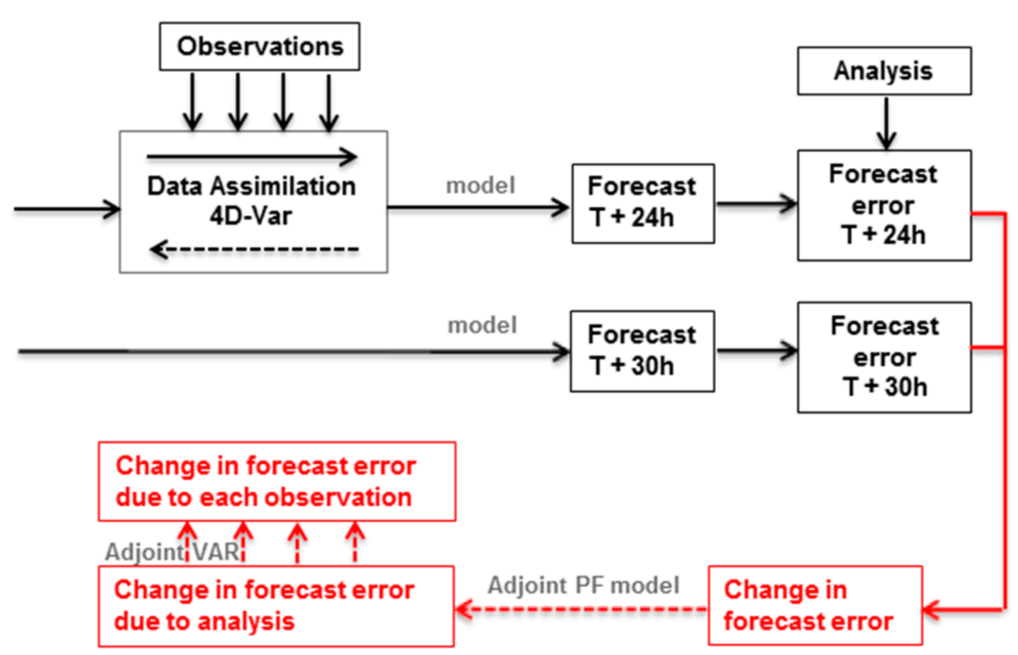
2.1. Essentials of the Forecast Sensitivity to Observation Method
2.2. Experimental Design
- -
- Sequential number of observation;
- -
- The observation value;
- -
- The value of innovation (the difference between observation and background values);
- -
- Sensitivity of the forecast to observation;
- -
- Latitude and longitude of observation;
- -
- Pressure level of observation (in hPa);
- -
- Indicator of the instrument type (radiosonde, surface station, wind profiler);
- -
- Indicator of the observation variable type (temperature, moisture, pressure, horizontal wind components);
- -
- The time offset of the observation from the analysis time;
- -
- Observation error variance;
- -
- WMO (World Meteorological Organization) station identification number;
- -
- Satellite identifier, satellite instrument and channel number.
3. Results
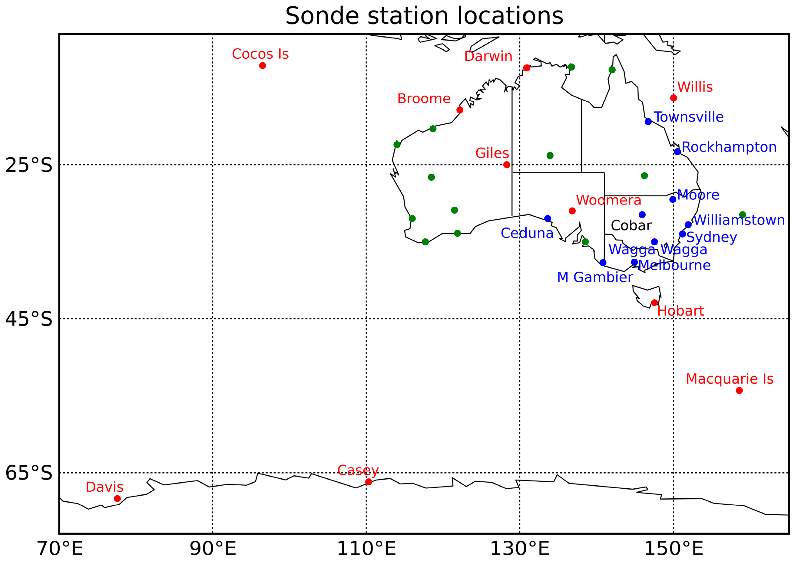
3.1. Observation Impacts of the Australian Sonde Network
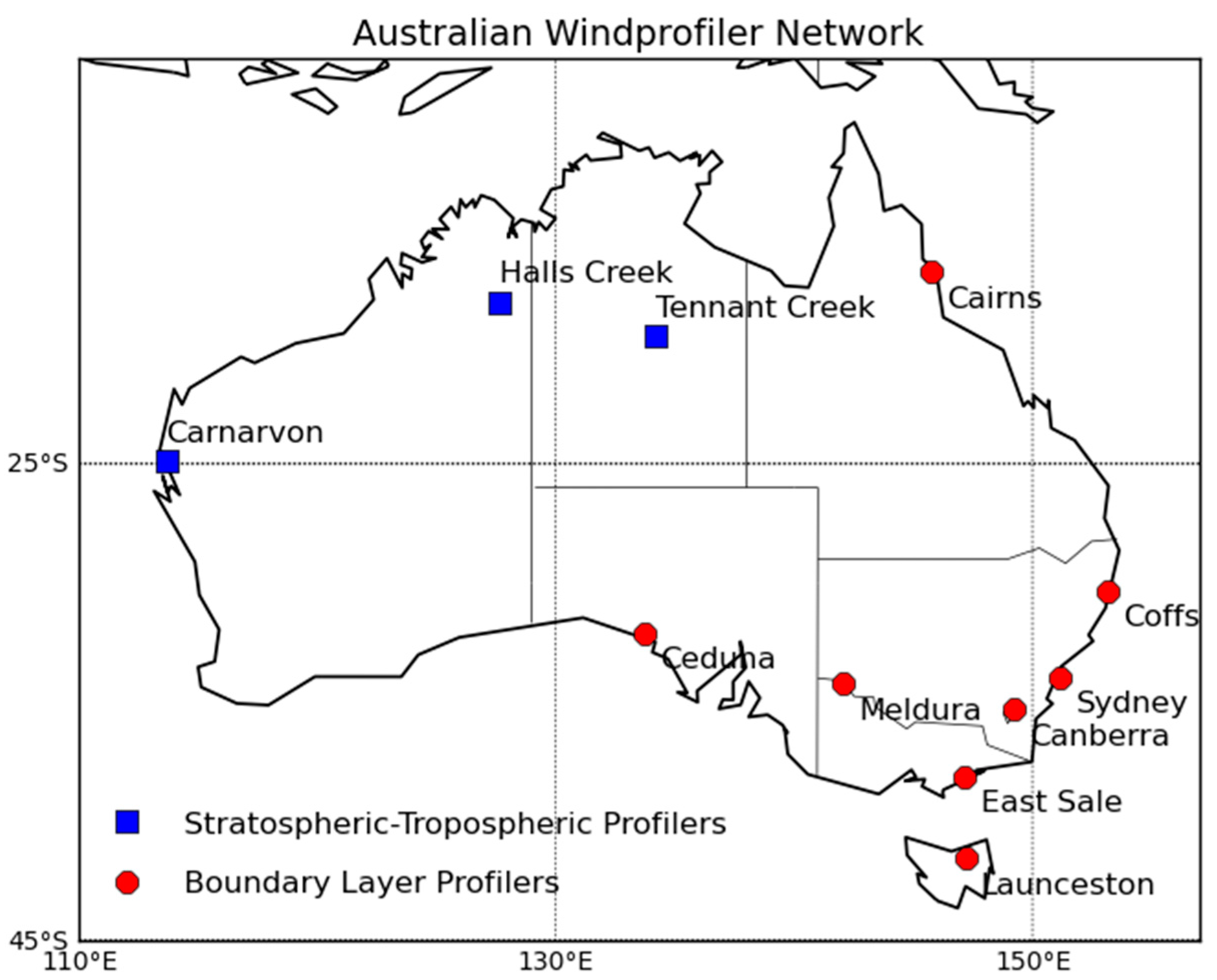
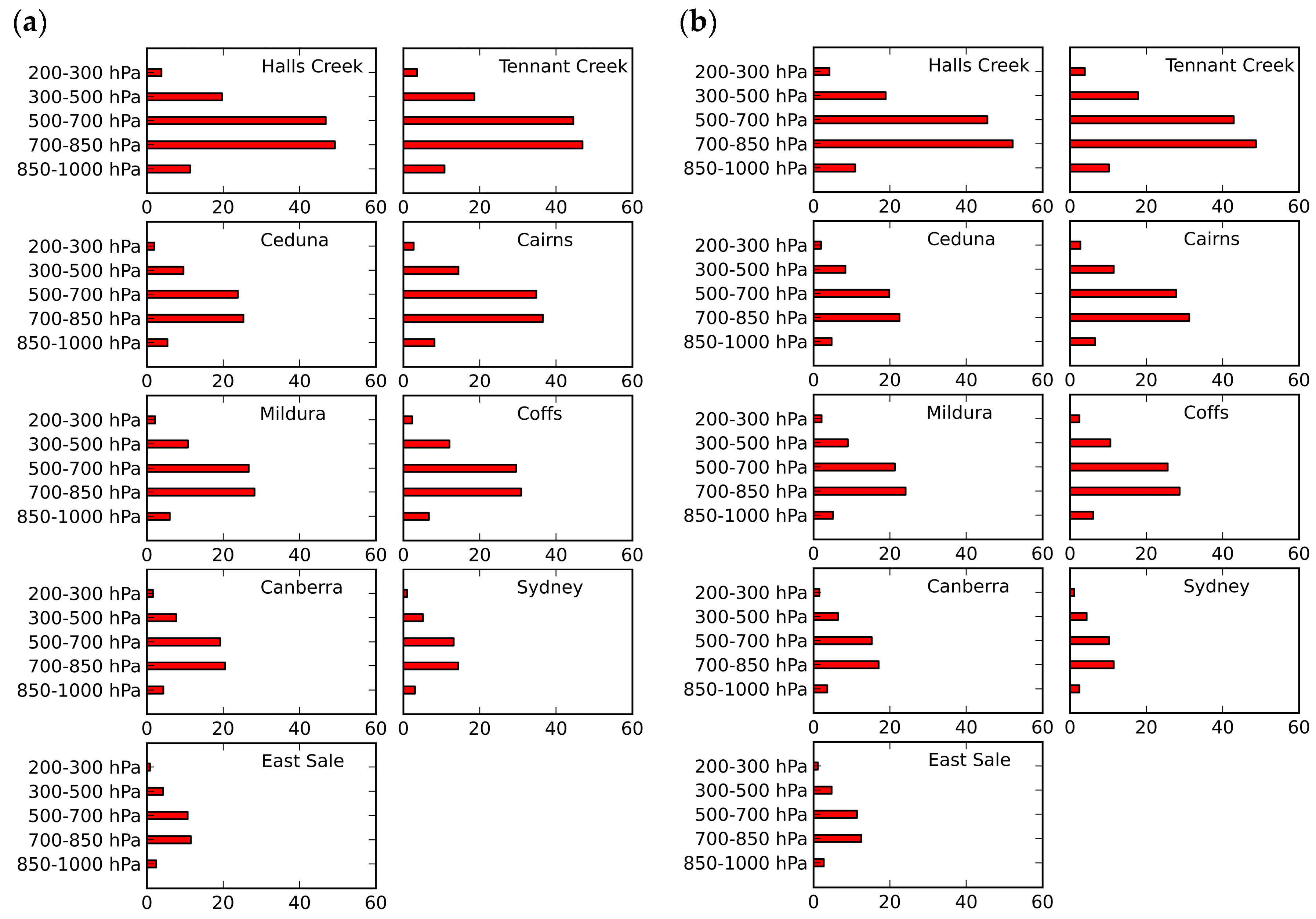
3.2. Observation Impacts of Australian Wind Profilers
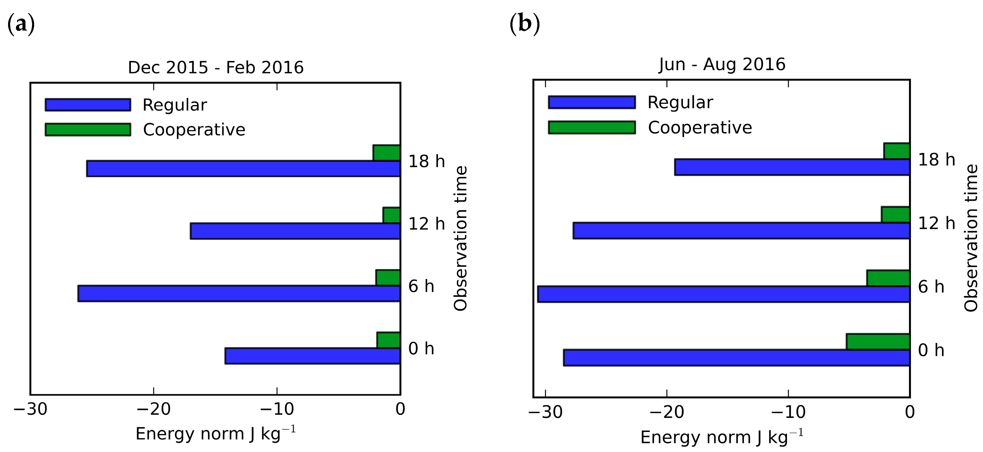
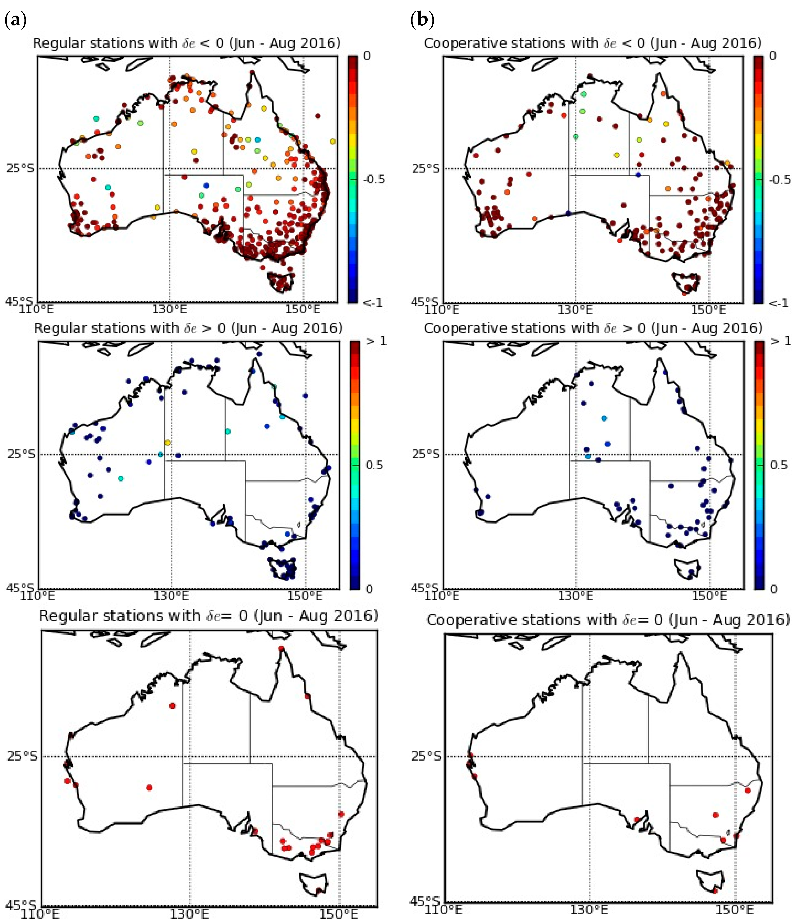
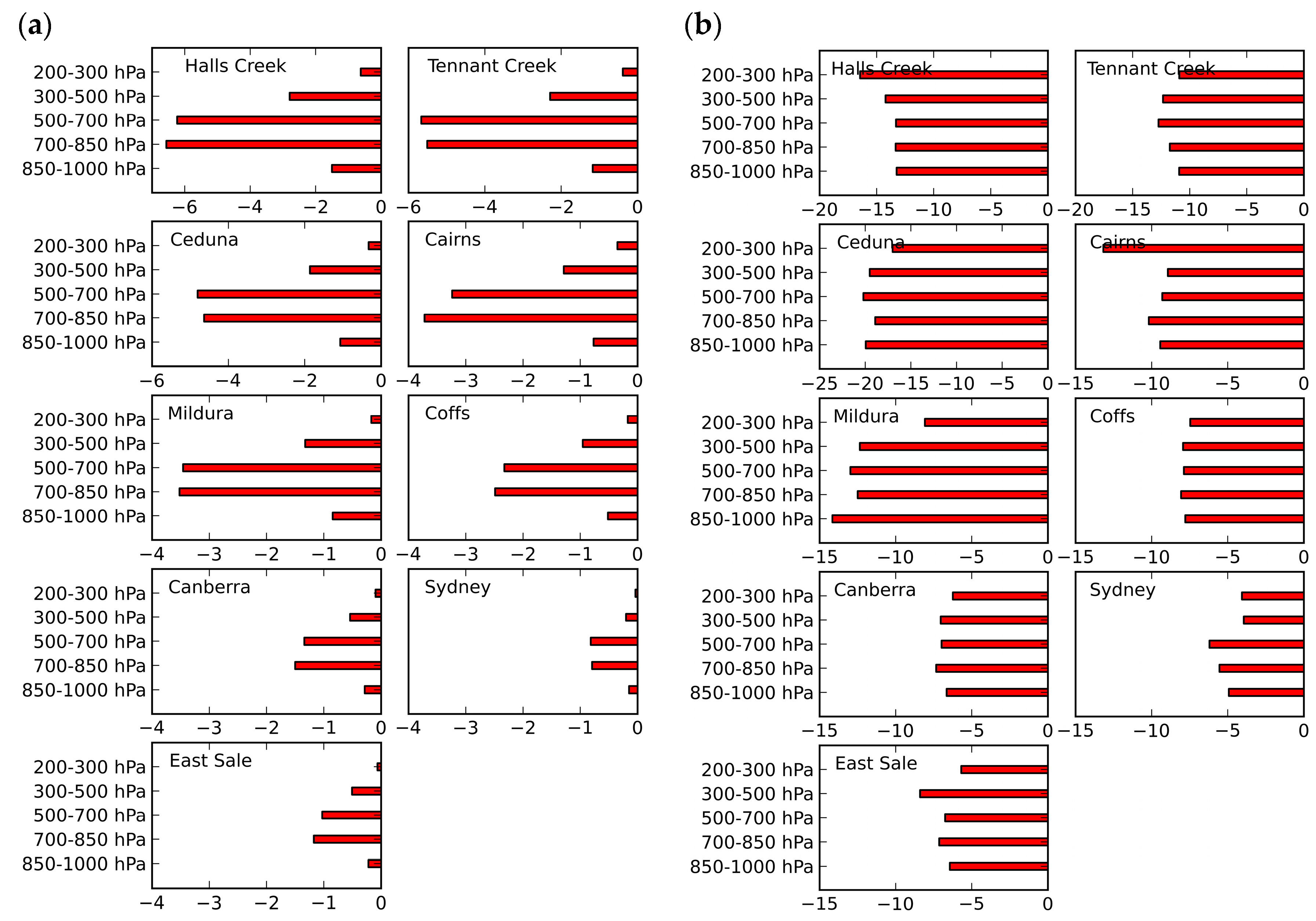
3.3. Observation Impacts of Australian Synoptic Observations
- (a)
- The need for observations of particular types;
- (b)
- How well a location represents the surroundings;
- (c)
- Availability of land, observers (if required) and infrastructure;
- (d)
- The presence of other stations in the area.
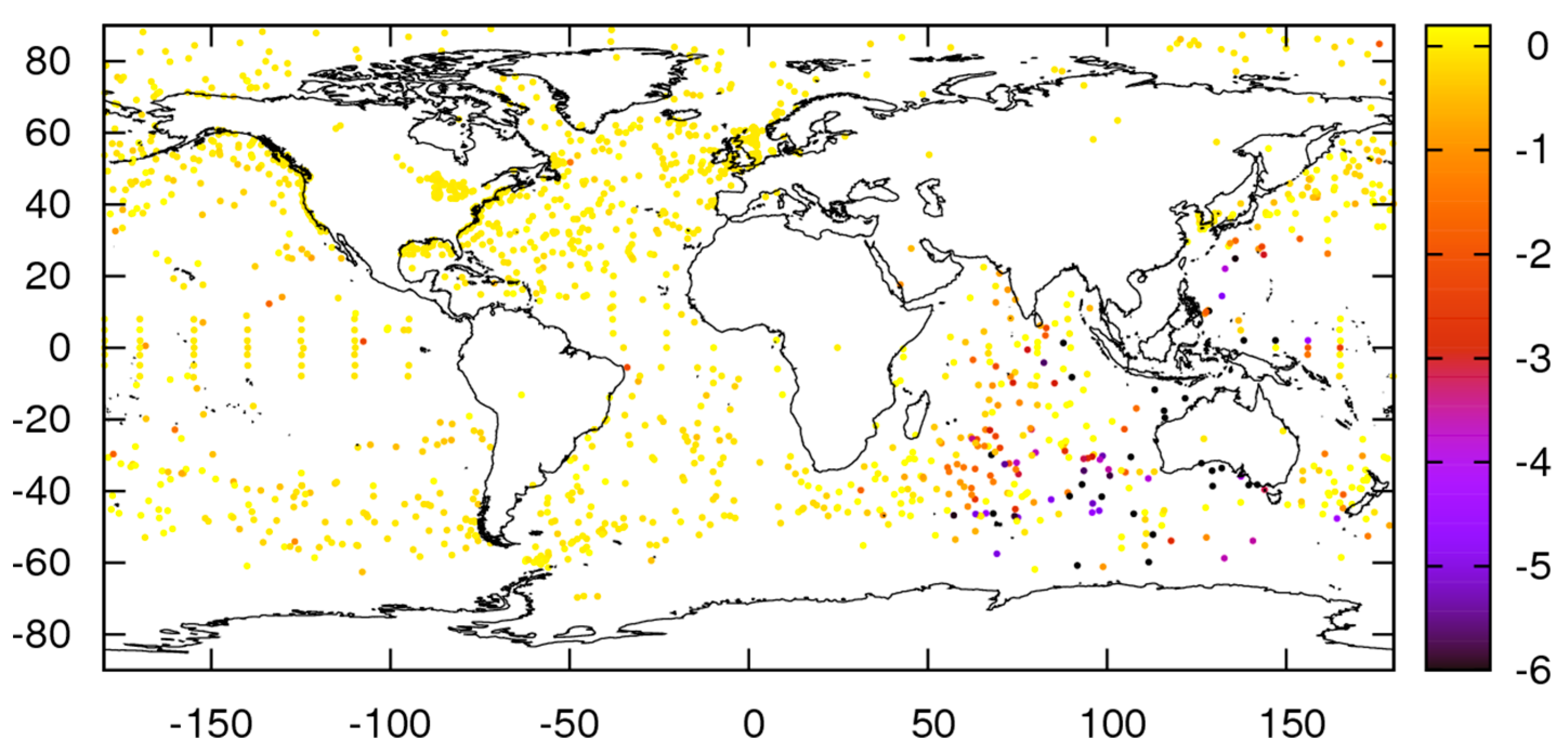
3.4. Observation Impacts from Buoys
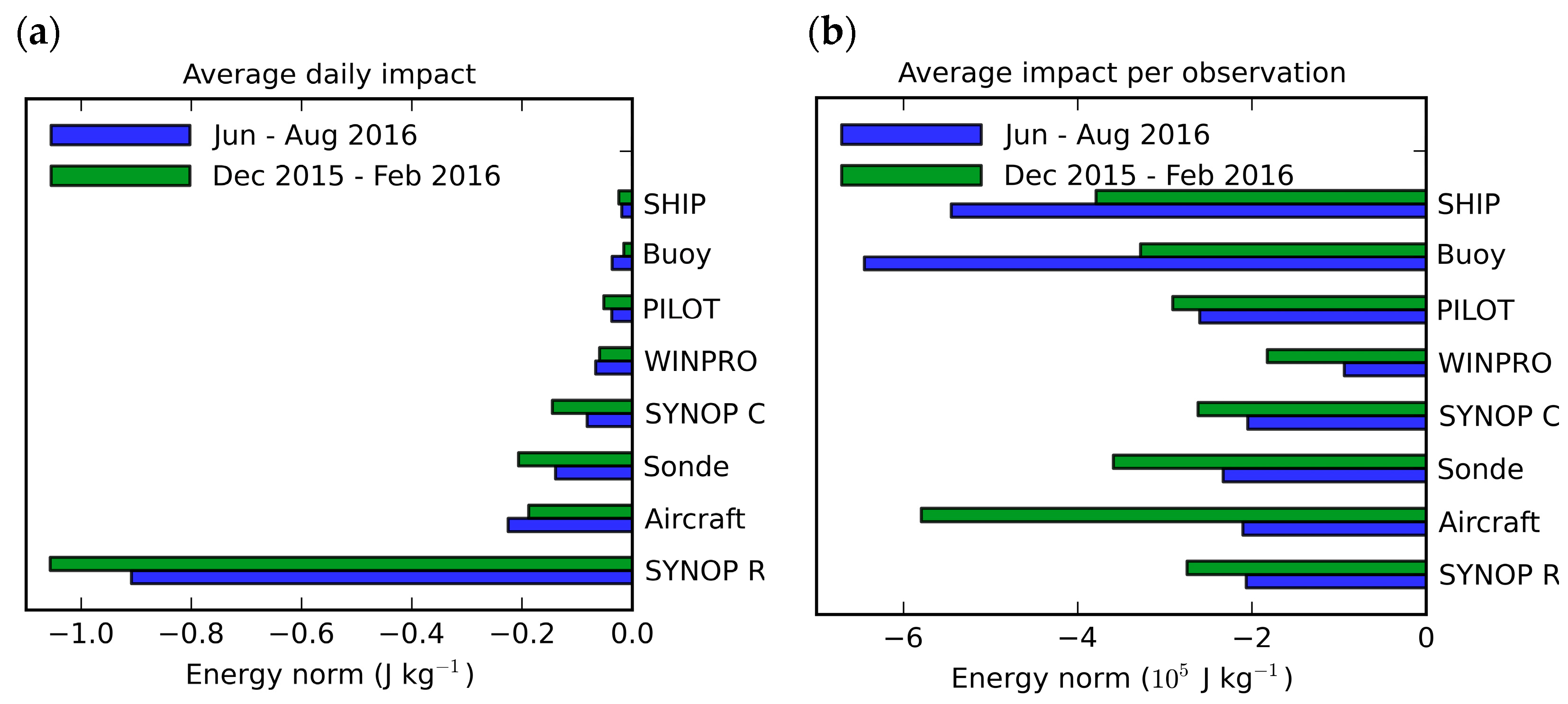
3.5. Comparison of Observation Impacts of Each In Situ Observation Type
4. Discussion and Conclusions
Acknowledgments
Author Contributions
Conflicts of Interest
References
- Puri, K.; Dietachmayer, G.; Steinle, P.; Dix, M.; Rikus, L.; Logan, L.; Naughton, M.; Tingwell, C.; Xiao, Y.; Barras, V.; et al. Implementation of the initial ACCESS numerical weather prediction system. Aust. Meteorol. Oceanogr. J. 2013, 63, 265–284. [Google Scholar] [CrossRef]
- Kelly, G.; Thépaut, J.-N. Evaluation of the impact of the space component of the Global Observing System through Observing System Experiments. ECMWF Newsl. 2007, 113, 16–28. [Google Scholar]
- Kelly, G.; Bauer, P.; Geer, A.J.; Lopez, P.; Thépaut, J.-N. Impact of SSM/I observations related to moisture, clouds and precipitation on global NWP forecast skill. Mon. Weather Rev. 2007, 136, 2713–2726. [Google Scholar] [CrossRef]
- Marseille, G.J.; Stoffelen, A.; Barkmeijer, J. Sensitivity Observing System Experiment (SOSE)—A new effective NWP-based tool in designing the global observing system. Tellus A 2008, 60, 216–233. [Google Scholar] [CrossRef]
- Gelaro, R.; Zhu, Y. Examination of observation impacts derived from observing system experiments (OSEs) and adjoint models. Tellus A 2009, 61, 179–193. [Google Scholar] [CrossRef]
- Bauer, P.; Radnóti, G. Study on Observing System Experiments (OSEs) for the Evaluation of Degraded EPS/Post-EPS Instrument Scenarios; Report Available from ECMWF; ECMWF: Reading, UK, 2009; p. 99. [Google Scholar]
- Masutani, M.; Schlatter, T.W.; Erico, R.M.; Stoffen, A.; Andersson, E.; Lahoz, W.; Woollen, J.S.; Emmitt, G.D.; Riishøjgaard, L.-P.; Lord, S.J. Observing System Simulation Experiments. In Data Assimilation; Lahoz, W., Khattatov, B., Menard, R., Eds.; Springer: Berlin/Heidelberg, Germany, 2010; pp. 647–679. [Google Scholar]
- Langland, R.H.; Baker, N.L. Estimation of observation impact using the NRL atmospheric variational data assimilation adjoint system. Tellus A 2004, 56, 189–201. [Google Scholar] [CrossRef]
- Le Dimet, F.-X.; Talagrand, O. Variational algorithms for analysis and assimilation of meteorological observations: Theoretical aspects. Tellus 1986, 38A, 97–110. [Google Scholar] [CrossRef]
- Courtier, P.; Thepaut, J.-N.; Hollingsworth, A. A strategy for operational implementation of 4D-Var, using an incremental approach. Q. J. R. Meteorol. Soc. 1994, 120, 1367–1387. [Google Scholar] [CrossRef]
- Baker, N.; Daley, R. Observation and background adjoint sensitivity in the adaptive observation targeting problem. Q. J. R. Meteorol. Soc. 2000, 126, 1434–1454. [Google Scholar] [CrossRef]
- Errico, M.R. Interpretations of an adjoint-derived observational impact measure. Tellus A 2007, 59, 273–276. [Google Scholar] [CrossRef]
- Daescu, D.N. On the deterministic observation impact guidance: A geometrical perspective. Mon. Weather Rev. 2009, 137, 3567–3574. [Google Scholar] [CrossRef]
- Daescu, D.N. On the sensitivity equations of four-dimensional variational (4D-Var) data assimilation. Mon. Weather Rev. 2008, 136, 3050–3065. [Google Scholar] [CrossRef]
- Daescu, D.N.; Todling, R. Adjoint estimation of the variation in a model functional output due to assimilation of data. Mon. Weather Rev. 2009, 137, 1705–1716. [Google Scholar] [CrossRef]
- Sandu, A.; Daescu, D.N.; Carmichael, G.R.; Chai, T. Adjoint sensitivity analysis of regional air quality models. J. Comput. Phys. 2005, 204, 222–252. [Google Scholar] [CrossRef]
- Tremolet, Y. Computation of observation sensitivity and observation impact in incremental variational data assimilation. Tellus A 2008, 60A, 964–978. [Google Scholar] [CrossRef]
- Cioaca, A.; Sandu, A.; de Sturler, E. Efficient methods for computing observation impact in 4D-Var data assimilation. Comput. Geosci. 2013, 17, 975–990. [Google Scholar] [CrossRef]
- Cardinali, C. Monitoring the observation impact on the short-range forecast. Q. J. R. Meteorol. Soc. 2009, 135, 239–250. [Google Scholar] [CrossRef]
- Lorenc, A.C.; Marriott, R.T. Forecast sensitivity to observations in the Met Office Global numerical weather prediction system. Q. J. R. Meteorol. Soc. 2014, 140, 209–224. [Google Scholar] [CrossRef]
- Rawlins, F.; Ballard, S.P.; Bovis, K.J.; Clayton, A.M.; Li, D.; Inverarity, G.W.; Lorenc, A.C.; Payne, T.J. The Met Office global 4-dimensional data assimilation system. Q. J. R. Meteorol. Soc. 2007, 133, 347–362. [Google Scholar] [CrossRef]
- Walters, D.; Boutle, I.; Brooks, M.; Melvin, T.; Stratton, R.; Vosper, S.; Wells, H.; Williams, K.; Wood, N.; Allen, T.; et al. The Met Office Unified Model Global Atmosphere 6.0/6.1 and JULES Global Land 6.0/6.1 configurations. Geosci. Model Dev. 2017, 10, 1487–1520. [Google Scholar] [CrossRef]
- Auligné, T.; Xiao, Q. Adjoint Sensitivity and Observation Impact. UCAR 2009. Available online: http://www2.mmm.ucar.edu/wrf/users/workshops/WS2009/presentations/2A-05.pdf (accessed on 12 April 2017).
- BNOC Operational Bulletin No. 105, 16 March 2016: “APS2 Upgrade to the ACCESS-G Numerical Weather Prediction System”. Available online: http://www.bom.gov.au/australia/charts/bulletins/APOB105.pdf (accessed on 1 June 2017).
- Dolman, B.; Reid, I.; Kane, T. The Australian Wind Profiler Network. In Proceedings of the WMO Technical Conference on Meteorological and Environmental Instruments and Methods of Observation (CIMO TECO 2016), Madrid, Spain, 27–30 September 2016. [Google Scholar]
- World Meteorological Organisation (WMO). Manual on Codes International Codes Volume I.2 Annex II to the WMO Technical Regulations Part B—Binary Codes. 2016. Available online: https://library.wmo.int/opac/doc_num.php?explnum_id=3421 (accessed on 7 December 2017).
- Errico, M.R. What is an adjoint model? Bull. Am. Met. Soc. 1997, 78, 2577–2591. [Google Scholar] [CrossRef]
- Ingleby, N.B. The statistical structure of forecast errors and its representation in the Met Office global three-dimensional variational data assimilation system. Q. J. R. Meteorol. Soc. 2001, 127, 209–231. [Google Scholar] [CrossRef]
- Seaman, R.; Bourke, W.; Steinle, P.; Hart, T.; Embery, G.; Naughton, M.; Rikus, L. Evolution of the Bureau of Meteorology’s Global Assimilation and Prediction System. Part 1: Analysis and initialisation. Aust. Meteor. Mag. 1995, 44, 1–18. [Google Scholar]
- Bourke, W.; Hart, T.; Steinle, P.; Seaman, R.; Embery, G.; Naughton, M.; Rikus, L. Evolution of the Bureau of Meteorology’s Global Assimilation and Prediction System. Part 2: Resolution enhancements and case studies. Aust. Meteor. Mag. 1995, 44, 19–40. [Google Scholar]
- Seaman, R.S. Which Australian rawinsonde stations most influence wind analysis? Aust. Meteorol. Mag. 2007, 56, 285–289. [Google Scholar]
- Seaman, R.S. Monitoring a data assimilation system for the impact of observations. Aust. Meteorol. Mag. 1994, 43, 41–48. [Google Scholar]


| Data Period | From 00Z 1 September 2015 to 00Z 31 December 2016 |
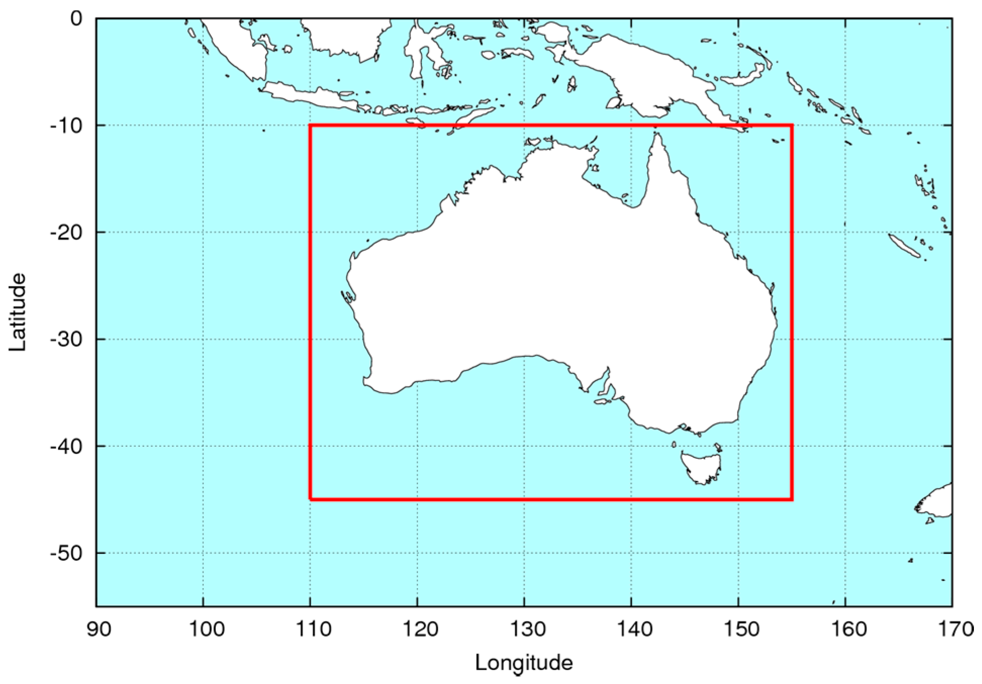
| Impact Measure | 24-h forecast error reduction on the moist energy norm calculated from the surface to 150 hPa level over the Australian region. |
| NWP System | Operational version of the Bureau of Meteorology NWP system, APS-2, with the resolution of N512 for the forecasting model and N216 for the inner loop of 4D-Var, in horizontal, and 70 levels in vertical. The adjoint of PF includes the moist physics. |
| Data ID | Data Type | Information |
|---|---|---|
| SYNOP | Surface observations from land-based weather stations | T, u, v, Rh, ps |
| SHIP | Surface observations from ships and oil rigs | T, u, v, Rh, ps |
| TEMP | Upper air observations by radiosondes | T, u, v, Rh, ps |
| PILOT | Upper air observations by radiosondes or pilot balloons released from land stations | u, v |
| WINPRO | Upper air wind profile observations | u, v |
| Aircraft | Aircraft observations | T, u, v |
| BUOY | Sea surface observations from drifting and moored buoys | T, ps |
| Rank | Station | Latitude (S) | Longitude (E) | Relative Impact | |
|---|---|---|---|---|---|
| 1 | 89611 | Casey (Antarctic) | 66°17′ | 110°31′ | 1.00 |
| 2 | 89571 | Davis (Antarctic) | 68°34′ | 77°58′ | 0.95 |
| 3 | 89564 | Mawson (Antarctic) | 67°36′ | 62°52′ | 0.94 |
| 4 | 94998 | Macquarie Island | 54°30′ | 158°57′ | 0.83 |
| 5 | 94120 | Darwin | 12°25′ | 130°53′ | 0.69 |
| 6 | 94461 | Giles Met Office | 25°02′ | 128°17′ | 0.69 |
| 7 | 94975 | Hobart | 42°50′ | 147°30′ | 0.52 |
| 8 | 94299 | Willis Island | 16°18′ | 149°59′ | 0.49 |
| 9 | 94203 | Broome Airport | 17°57′ | 122°14′ | 0.45 |
| 10 | 96996 | Cocos Island | 12°11′ | 96°50′ | 0.45 |
| 11 | 94659 | Woomera Aero | 31°09′ | 136°49′ | 0.41 |
| 12 | 94326 | Alice Spring | 23°48′ | 133°53′ | 0.39 |
| 13 | 94995 | Lord Howe Island | 31°32′ | 159°04′ | 0.38 |
| 14 | 94150 | Gove Aero | 12°17′ | 136°49′ | 0.37 |
| 15 | 94302 | Learmonth Aero | 22°14′ | 114°05′ | 0.32 |
| 16 | 94170 | Weipa Aero | 12°41′ | 141°55′ | 0.28 |
| 17 | 94610 | Perth Aero | 31°56′ | 115°58′ | 0.25 |
| 18 | 94510 | Charleville Aero | 26°25′ | 146°16′ | 0.25 |
| 19 | 94672 | Adelaide | 34°57′ | 138°32′ | 0.25 |
| 20 | 94637 | Kalgoorlie-Boulder | 30°47′ | 121°27′ | 0.21 |
| 21 | 94638 | Esperance | 33°50′ | 121°53′ | 0.19 |
| 22 | 94802 | Albany Aero | 34°56′ | 117°48′ | 0.18 |
| 23 | 94312 | Port Hedland Aero | 20°22′ | 118°38′ | 0.17 |
| 24 | 94430 | Meekatharra Aero | 26°37′ | 118°33′ | 0.15 |
| 25 | 94866 | Melbourne | 37°40′ | 144°51′ | 0.13 |
| 26 | 94527 | Moree Aero | 29°29′ | 149°50′ | 0.10 |
| 27 | 94294 | Townsville | 19°15′ | 146°46′ | 0.10 |
| 28 | 94711 | Cobar Mo | 31°29′ | 145°50′ | 0.10 |
| 29 | 94776 | Williamstown | 32°48′ | 151°50′ | 0.10 |
| 30 | 94821 | Mount Gambier Aero | 37°44′ | 140°47′ | 0.10 |
| 31 | 94374 | Rockhampton Aero | 23°23′ | 150°29′ | 0.07 |
| 32 | 94653 | Ceduna | 32°08′ | 133°42′ | 0.07 |
| 33 | 94910 | Wagga Wagga | 35°10′ | 147°27′ | 0.04 |
| 34 | 94767 | Sydney | 33°56′ | 151°10′ | 0.01 |
© 2018 by the authors. Licensee MDPI, Basel, Switzerland. This article is an open access article distributed under the terms and conditions of the Creative Commons Attribution (CC BY) license (http://creativecommons.org/licenses/by/4.0/).
Share and Cite
Soldatenko, S.; Tingwell, C.; Steinle, P.; Kelly-Gerreyn, B.A. Assessing the Impact of Surface and Upper-Air Observations on the Forecast Skill of the ACCESS Numerical Weather Prediction Model over Australia. Atmosphere 2018, 9, 23. https://doi.org/10.3390/atmos9010023
Soldatenko S, Tingwell C, Steinle P, Kelly-Gerreyn BA. Assessing the Impact of Surface and Upper-Air Observations on the Forecast Skill of the ACCESS Numerical Weather Prediction Model over Australia. Atmosphere. 2018; 9(1):23. https://doi.org/10.3390/atmos9010023
Chicago/Turabian StyleSoldatenko, Sergei, Chris Tingwell, Peter Steinle, and Boris A. Kelly-Gerreyn. 2018. "Assessing the Impact of Surface and Upper-Air Observations on the Forecast Skill of the ACCESS Numerical Weather Prediction Model over Australia" Atmosphere 9, no. 1: 23. https://doi.org/10.3390/atmos9010023