A Robust Non-Gaussian Data Assimilation Method for Highly Non-Linear Models


1
Applied Math and Computational Science Laboratory, Department of Computer Science, Universidad del Norte, Barranquilla 080001, Colombia
2
Department of Computer Science, Willamette University, 900 State Street, Salem, OR 97301, USA
*
Author to whom correspondence should be addressed.
Atmosphere 2018, 9(4), 126; https://doi.org/10.3390/atmos9040126
Submission received: 5 January 2018
/
Revised: 14 March 2018
/
Accepted: 20 March 2018
/
Published: 26 March 2018
(This article belongs to the Special Issue Efficient Formulation and Implementation of Data Assimilation Methods)
Abstract
:In this paper, we propose an efficient EnKF implementation for non-Gaussian data assimilation based on Gaussian Mixture Models and Markov-Chain-Monte-Carlo (MCMC) methods. The proposed method works as follows: based on an ensemble of model realizations, prior errors are estimated via a Gaussian Mixture density whose parameters are approximated by means of an Expectation Maximization method. Then, by using an iterative method, observation operators are linearized about current solutions and posterior modes are estimated via a MCMC implementation. The acceptance/rejection criterion is similar to that of the Metropolis-Hastings rule. Experimental tests are performed on the Lorenz 96 model. The results show that the proposed method can decrease prior errors by several order of magnitudes in a root-mean-square-error sense for nearly sparse or dense observational networks.
1. Introduction
Data Assimilation is the process of optimally combining the imperfect numerical forecast states and imperfect observations to better estimate the state of a system that evolves according to some model operator [1,2,3],
where, is an imperfect numerical model that evolves the states, n is the number of model components. One example of could be a model that mimics the ocean and/or the atmosphere dynamics. In traditional DA settings, prior errors are described by Gaussian distributions,
where and is the background state and the background error covariance matrix, respectively. This assumption has plenty of computational benefits, for instance, by assuming Gaussian errors in the prior and the observations, Kalman-like updates can be performed in order to compute posterior (error) moments. However, in the context of geophysics, model dynamics can be highly non-linear and therefore, Gaussian Mixture Models (GMM) [4,5] can be used to capture our prior knowledge about the error dynamics:
where, for the k-th mixture component, is the mean, is the background error covariance, and is the prior weight, for . These weights can be estimated, for instance, using the Expectation Maximization algorithm [6,7,8]. In sequential methods, it is common to assume Gaussian errors over observations ,
where m is the number of observed components from the model state, is the data error covariance matrix, and is the observation mapping operator. When the operator is linear, the posterior error distribution can be described by a GMM [9] as well:
with updated weights , centroids , and covariances , for , which account for the observation (3). It can be noted that, for the k-th mixture component, the posterior mode can be obtained by means of a 3D-Var optimization problem:
where
Under linear assumptions, can be estimated by means of, for instance, an EnKF updating formula. However, for non-linear observation operators, such expression can fail to obtain reasonable estimates of posterior modes and therefore, other alternatives such as sampling methods are employed. For instance, Monte-Carlo based methods are commonly utilized in order to relax the Gaussian assumption in the observational errors. Thus, we propose an efficient sampling method to draw samples from the posterior distribution (4) using cost functions of the form (6). In general, the method works as follows: for a fixed number of clusters, a GMM is fitted with the EM method, then, for each prior component, samples are drawn along steepest descent approximations of the 3D-Var cost function; these samples are accepted/rejected based on the Metropolis–Hastings rule. Besides, background error correlations are estimated based on a modified Cholesky decomposition in order to perform implicit localization and to reduce the impact of sampling errors, a major concern in the context of DA.
This paper is organized as follows: Section 2 discusses EnKF formulations and sampling methods for relaxing Gaussian assumptions in prior and observation errors. Section 3 presents an EnKF formulation based on GMM and MCMC (Markov-Chain-Monte-Carlo) for computing posterior modes together with error statistics; the computational cost of the method is estimated as well. In Section 4, experimental tests are performed on the Lorenz-96 model and non-linear observation operators; conclusions are finally stated in Section 5.
2. Preliminaries
2.1. Ensemble Kalman Filters Based on Modified Cholesky Decomposition
In sequential Data Assimilation (DA), under prior Gaussian assumptions, a well-known filter is the ensemble Kalman filter (EnKF) [10,11]. In EnKF, using an ensemble of model realizations,
the hyper-parameters of the error distribution,
are estimated as:
and
where is the background state, is the background error covariance matrix, N is the ensemble size, denotes the e-th ensemble member, for . is known as the ensemble mean, and is the ensemble covariance matrix. The matrix of member deviations reads
and is a vector of consistent dimension whose components are all ones. When an observation becomes available, in the stochastic EnKF, the analysis ensemble can be estimated as follows:
where is the matrix of scaled innovations on the observations. The columns of are formed by samples from a m-th dimensional standard Normal distribution. is the linearized observation operator (with the linearization performed about the background state) also known as the Jacobian matrix of at the background state, and is the analysis covariance matrix:
In operational DA, ensemble sizes are several orders of magnitude smaller than the model dimensions () and as a consequence, the covariance matrix is commonly rank-deficient. This implies that (7g) cannot be directly computed and even though equivalent updating formulas which avoid the calculation can be found in the literature, sampling errors can still impact the quality of the analysis corrections. In practice, localization methods are often used to artificially increase the degrees of freedom of and to mitigate the impact of sampling errors [12,13,14,15]. An efficient EnKF implementation which accounts for implicit localization during the assimilation step is the EnKF method based on a modified Cholesky decomposition (EnKF-MC) [16]. In this filter, the vanilla covariance (7d) is replaced by the Bickel and Levina estimator [17]:
where is a lower triangular matrix whose diagonal elements are all ones. Its non-zero sub-diagonal elements are computed by fitting models of the form:
In which denotes the predecessors of the i-th grid component for some labelling of model components, stands for the i-th row of the matrix (7e), and, as an assumption, follows a zero-mean Normal distribution with uncorrelated errors of unknown variance . Likewise, is a diagonal matrix whose diagonal elements are given by the reciprocal variances of the residuals in (8b):
Similar to (7f), the analysis ensemble can be built as,
where an estimate of the analysis covariance is:
Matrix-free implementations of the EnKF-MC are currently proposed in the literature, for instance, the Posterior EnKF (P-EnKF) [18,19] exploits the special structure of (8a) in order to estimate Cholesky factors of the posterior precision covariance (8e). Consider
where , for , is the o-th column of matrix , the updating process can be done via a sequence of rank-one updates over the prior Cholesky factors:
where and are the Cholesky factors of . Having a posterior precision in the form , an estimate of the posterior ensemble can be easily built:
where is given by the solution of a lower triangular linear system:
In spite of EnKF implementations well-recognized by the DA community, the Gaussian assumption (7b) can be easily broken when the numerical model dynamics (1) are highly non-linear. For this reason, one prefers to use a different model to describe the prior error distribution. A Gaussian Mixture Model is frequently used to relax the Gaussian assumption over the forecast distribution [20,21,22,23].
2.2. Gaussian Mixture Models Based Filters
In EnKF formulations based on Gaussian Mixture Models (GMM), the prior error distribution (7b) is replaced by a mixture of Gaussian distributions (2). Based on this general idea, many methods have been proposed in the current literature in order to deal with highly non-linear dynamics of, for instance, operational DA models. These methods rely on the assumption that GMM models can approximate arbitrary density functions. GMM components are commonly fitted by using the Expectation Maximization (EM) algorithm [24]. As the name implies, this iterative method works in two recursive steps: Expectation (E) and Maximization (M). For a fixed number of clusters K, at iteration p, during the E-step, the probability of representativeness of each ensemble member is computed with regard to clusters:
which allows us to approximate the k-th weight for the prior mixture component:
GMM components are updated during the M-step:
where , the matrix of intra-cluster deviations reads
Under linear assumptions, GMM-EnKF formulations exploit the fact that a Gaussian distribution is conjugate of a GMM. Thus, posterior components can be computed as results of performing Kalman-like updates over prior weights, centroids, and covariances as follows:
and
where , and . This computationally friendly property is exploited by filters such as the Non-linear Bayesian Estimator (N-BE) [25] and the Gaussian Mixture Ensemble Filter [26,27]. In [28] the N-BE is enhanced by using the Bayesian Information Criteria (BIC)
in order to choose the number of components for the GMM, where denotes a Normal probability density function with parameters and , respectively. This is possible, as well, by other means, for instance in the GMM-EnKF filter proposed by Smith in [29], the number of mixture components relies on the Akaie’s Information Criteria (AIC)
The BIC and the AIC are common methods for choosing the number of parameters in GMM but, information criteria based methods are poorly suited for selecting a model with a good out-of-sample fit in model-rich environments [30,31]. Besides, these methods are only valid for sample size N much larger than the number K of parameters, which can be difficult in the DA context.
Other methods such as Particle Filters (PFs) [32] are available in the literature in order to attack non-Gaussian DA problems. These methods are a good-choice from a theoretical point of view. Unfortunately, in practice, PFs do suffer from a degeneracy problem [33] (Section 1.4) and even more, many challenges have to be overcome before they can be considered under operational DA scenarios [34,35]. For these reasons, PFs are not considered any further in this paper.
3. Proposed Method
In this section, we develop an efficient Gaussian mixture ensemble Kalman filter implementation based on Markov-Chain-Monte-Carlo (GM-EnKF-MCMC) for non-Gaussian data assimilation. We describe in detail how hyper-parameters are computed as well as how observations are digested for the GM-EnKF-MCMC. Lastly, we briefly discuss how posterior ensembles are built.
3.1. Estimation of Hyper-Parameters—EM Method
Consider an ensemble of model realizations
where stands for the e-th ensemble member, for . To estimate the hyper-parameters of the prior error distribution, we use the EM method to fit a GMM with K components. Instead of estimating background error covariances , for , for the mixture components, we do prefer to estimate precision covariances due to their computational benefits. For instance, in the context of Normal distributions, probabilities are computed based on precision covariances which would require the inversion of large matrices when background error covariances are fitted during EM steps. Besides, by using the modified Cholesky decomposition for computing the precision covariances, we can exploit their special structures in order to obtain huge savings in terms of memory usage and to reduce the computational cost of matrix-vector products among iterations.
The proposed EM method works as follows: for a given number of clusters K, we choose K random members from the ensemble (13) in order to set the initial mixture centroids while the initial precision covariances are all equal to the precision covariance of the ensemble (8a). During the E-step, we compute the representativeness of each ensemble member regarding each cluster
where
The M-step updates the precision covariances as well as the background error states for each cluster. Consider the diagonal matrix of fuzzy weights,
the GMM centroids are updated as follows:
where . Likewise, the non-zero elements of (14b) are revised by fitting models of the form:
where is the i-th row of matrix
errors are assumed Normal distribution with zero mean and uncorrelated components of variance . Moreover, the diagonal entries of are estimated via the residuals of model (15c):
with . Note that whenever covariance inflation is desired before assimilation steps, the inflation factors can be applied to the matrix of member deviations with regard to centroids (15d). In this manner, the estimated precision covariances come already inflated. Once the EM steps are concluded (i.e., when a maximum number of iterations is reached), the prior error distribution is described by the GMM:
The special structure of the resulting precision covariances can be exploited in order to reduce the computational effort of drawing samples from the posterior error distribution as is discussed in the next section.
3.2. Sampling Method—Approaching the Posterior
In order to approximate samples from the posterior distribution (4), for each mixture component in (16), we use a Markov-Chain-Monte-Carlo (MCMC) approximation. Traditionally, Normal distributions are good candidates for proposing states, for instance, in our context, starting with and , at iteration , where v is a user-defined number of iterations, a state can be proposed as follows:
Or simply,
where is given by the solution of an upper triangular linear system:
and follows a standard Normal distribution. Nevertheless, in high-dimensional spaces such as those found in the context of operational DA, high-probability zones of posterior error distributions can be reached after a huge number of iterations. Thus, to overcome this situation, we proceed as follows: we linearize the observation operator about the current state ,
where is the Jacobian matrix of at , the cost function (6) can then be approximated by the quadratic cost function:
whose gradient reads,
By using this gradient, the proposal distribution (17) can be modified in such a manner that, samples along the (approximated) steepest descent direction of (6) have high probability of occurrence, that is,
where stands for an Uniform distribution on the interval . The value of can be tuned according to the degree of the observation operator. For instance, for a linear observation operator, can be set as since the gradient of (6) and (18a) are the same. When observation operators are highly non-linear, since Taylor based approximations suffer from myopia, a small step of such gradient must be taken and therefore, a good choice under this consideration is 1. Thus, an intuitive range for can be
In the absence of prior information about , one can choose 1. The main motivation for using gradient approximations is that, the subset of samples along the descent direction (19) can provide states which potentially maximize the posterior probability. Computationally speaking, no matrix inversion is needed in this context in order to propose states. The acceptance/rejection rule for the states (19) rely on the Metropolis-Hastings criterion which can be adapted as follows:
The observation operator is then linearized about and the overall process is repeated until some number of iterations is satisfied (or any other numerical condition). Putting it all together, the sampling procedure to compute the posterior modes is in the following:
- Step 1
- Let , set , go to step 2.
- Step 2
- Set .
- Step 3
- Linearize about and compute the direction (18b).
- Step 4
- Compute via Equation (19).
- Step 5
- Set according to Equation (20).
- Step 6
- If set and go to step 3, set and go to step 7 otherwise.
- Step 7
- If go to step 1, go to step 8 otherwise.
- Step 8
- The posterior mode approximations read .
Note that, unlike MCMC methods based on Random-Walk, for each prior mode, this procedure does not return a chain but only the last state in . This sampling step can be replaced by an optimization method such as Trust Region [36,37,38] or Line Search [39,40]. However, in order for it to work, some regularities must be satisfied by the gradient approximation (18b) [41,42,43,44,45], for instance, smoothness, which in practice is not necessarily the case.
3.3. Building the Posterior Ensemble
Once the posterior modes are computed, posterior covariances within clusters can be estimated as follows:
Therefore, the analysis members can be computed as:
where is estimated via the likelihood ratio:
3.4. Computational Complexity
In this section, we estimate the number of long computations of the proposed method in order to assess its computational effort. We detail the number of computations of the GMM-EnKF-MCMC below, we avoid the use of iteration indexes for ease of reading:
- During the E-Step, the computations of weights (14a) depend on the calculation:From this step, given the special structure of , can be computed with no more than long computations where denotes the maximum number of non-zero elements across all rows in with . Likewise, the number of long computations in order to obtain is bounded by since is diagonal. Thus, since there are K clusters, each E-step has the following operation counting:
- During the M-step, updating the centroids (15b) can be performed with no more than since has only n components different from zero (the diagonal ones), the least square solution of (15c) is bounded by calculations since there are n model components, and the cost of (15e) is bounded by since the multiplication of coefficients and model components is constrained to the neighbourhood of each model component. The computational effort of this method is then estimated as follows:
- During the sampling procedure, the gradient (18b) can be efficiently computed as follows:Given the special structure of , and can be computed with no more than , the computations in are bounded by since is diagonal. Thus, since this sampling method is performed v times, the computational effort of the sampling procedure reads,
- The posterior ensemble can be built (Section 3.3 [19]) with no more thanlong computations.
Assuming that the number of clusters and the number of iterations in the sampling process are much lower than the model dimension, based on Equation (22) the computational effort of the GMM-EnKF-MCMC reads,
which is linear with regard to the model resolution n.
3.5. Comparison of GM-EnKF-MCMC with Other Sampling Methods
In this section, we briefly compare the GM-EnKG-MCMC method with well-known filters from the literature: the Cluster Sampling Filter (CSF) [21], the Cluster Monte Carlo Implementation (CMCI) [46], and the Cluster Ensemble Kalman Filter (CEnKF) [29].
The CSF exploits the evolution of a system under Hamiltonian dynamics, for instance, based on Newton’s law it is possible to describe the dynamics of particles. Each particle is fully described by two components: the position and the velocity coordinates which are associated with model states and momentums (auxiliary variables), respectively. The performance of CSF relies on the proper choice of a mass matrix in order to describe the probability distribution of during the sampling process. Besides, numerical integrators which preserve Liouville’s Theorem are a must in order to obtain a proposal state . Some of those are the Verlet integrator [47] and the Leap-frog scheme [48]. A main difference between the GMM-EnKF-MCMC and the CSF is that, no auxiliary n-th dimensional vectors are required in our method during the sampling process. This can be convenient, for instance, under current operational DA systems. Besides, during the sampling process, the only parameter to be tuned in the GMM-EnKF-MCMC is in (17) while in the CSF method, as we mentioned before, proper choices of are required in order to speed-up the convergence of MCMC towards high-probability zones of the posterior. Besides, extra parameters may need to be tuned depending on the numerical integrator chosen in order to propose states during the sampling process.
In the CMCI, the background error distribution is approximated by a summation of Gaussian Kernels. These are selected using the method of Fukunaga [49] to form a continuous approximation to the random ensemble. By assuming linear observation operators, the posterior ensemble is Gaussian as well. Posterior members are drawn by sampling each of the components/kernels based on a set of calculated weights which account for the observation. As is pointed out by the authors, the CMCI is a very promising filter but, additional work is needed in order to extend its capabilities to more realistic scenarios. Moreover, this filter has been developed under Gaussian assumptions on the observations; such assumption is not required in the GMM-EnKF-MCMC.
The CEnKF is developed by assuming linear observation operators. Prior error distributions are described by GMM and its components are fitted by using the EM-method. This filter can fail to obtain reasonable estimates of posterior ensembles when non-linear observation operators are present during the assimilation of observations, as is typical in practice.
4. Experimental Settings
In this section, numerical tests are performed to assess the accuracy of the proposed filter. We use the Lorenz-96 model [50] as our surrogate model. The Lorenz-96 model is described by the following set of ordinary differential equations [51]:
where F is external force and is the number of model components. Periodic boundary conditions are assumed. When the model exhibits chaotic behavior, which makes it a relevant surrogate problem for atmospheric dynamics [52,53]. One time unit in the Lorenz-96 represents 7 days in real case. The experimental settings are described below:
- Starting with an initial random solution, a 4th order Runge Kutta method is employed in order to integrate it over a long time period from which initial condition is obtained.
- A perturbed background solution is formed at time by drawing a sample from the Normal distribution,This solution is then integrated for 10 time units (equivalent to 70 days) in order to obtain a background solution consistent with the dynamics of the numerical model.
- An initial perturbed ensemble is built about the background state by taking samples from the distribution,In order to make them consistent with the model dynamics, the ensemble members are propagated for 10 time units, from which the initial ensemble members are obtained. We create the initial pool of members. The actual solution is integrated over 20 more time units in order to place it at the beginning of the assimilation window.
- Two assimilation windows are proposed for the tests, both of them consist of observations. In the first assimilation window, observations are taken every 16 h (time step of 0.1 time units) while in the last one, observations are available every 50 h (time step of 0.3 time units). We denote by the elapsed time between two observations.
- The observational errors are described by the probability distribution,where the standard deviations of observational errors , and ℓ should be interpreted as time index. Random observation networks are formed at the different assimilation cycles. The space between observations will depend on the step size, for instance, in the first step size observations are available every 0.1 time units (16 h) while in the last one, observations are taken every 0.3 time units (50 h).
- We consider the non-linear observation operator [32]:where j denotes the j-th observed component from the model state. .
- We consider two percentages of observed components s from the model state .
- The radius of influence is set to while the inflation factor is set to 1.02 (a typical value).
- We propose two ensemble sizes for the benchmark . These members are randomly chosen from the pool for different experiments in order to form the initial ensemble for the assimilation window. Evidently, .
- The norm of errors are utilized as a measure of accuracy at the assimilation step ℓ,where and are the reference and the analysis solutions, respectively. The analysis state is obtained by a weighted combination of posterior centroids via the likelihood ratio (21b) in lieu of the posterior mean.
- The Root-Mean-Square-Error (RMSE) is used as a measure of performance. On average, on a given assimilation window,
Results for h, different ensemble sizes, and different values of are shown in Figure 1 in terms of L-2 error norms per assimilation step (25). Notoriously, the performance of the filter is improved as long as prior errors are described by a GMM (). This can be expected owing to the non-linear dynamics of the Lorenz-96 model. In addition, the performance of the GMM-EnKF-MCMC is not impacted by the degree of the observation operator. Both features make the proposed formulation attractive for DA systems where non-linear observation operators are the bridge for digesting observations and besides, non-linear dynamics are encapsulated in the numerical model. Moreover, for , there are less posterior errors than in prior and observations; this of course must be expected for full observational networks. In some cases, filter divergence is possible for (a single mode prior distribution). Assuming that spurious correlations are not impacting the analysis corrections, in this set of experiments, filter divergence can be seen as a consequence of one of two things: prior errors are not well fitted by a Gaussian distribution (the actual error distribution is multimodal) or inflation factors are not properly tuned. Regardless of the main cause, filter convergence is evident when a GMM describes the background error distribution. In Figure 2, results for , different ensemble sizes, and different values of are shown as well. Under this configuration, the accuracy of the GMM-EnKF-MCMC is slightly impacted by increments in . Filter convergence is rapidly achieved when the number of prior modes is larger than one. Despite the fact that filter divergence can be still for , interestingly, the proposed method does a reasonable estimation of the actual state of the system. In the linear case, this is not surprising, EnKF formulations are widely utilized in practice wherein Gaussian assumptions are commonly broken during assimilation steps. For non-linear observation operators , and Gaussian assumptions on the prior , the accuracy of the filter relies on the sampling procedure. As can be seen, under such assumptions, the proposed method is capable of obtaining good estimates of posterior error modes.
RMSE values () (26) in the log-scale are shown in the Table 1 and Table 2 for and , respectively. We group RMSE values by elapsed time between observations and number of observed components s. Notice that the performance of the filter can be improved when the number of prior modes is larger than one. This aligns with the highly non-linear (and chaotic) dynamics exhibited by the Lorenz 96 model which makes a single mode distribution insufficient to encapsulate all prior information. However, the GMM-EnKF-MCMC can be impacted when a large number of mixture components is utilized and in some cases, overfitting is possible, for instance, in Table 1, for and .
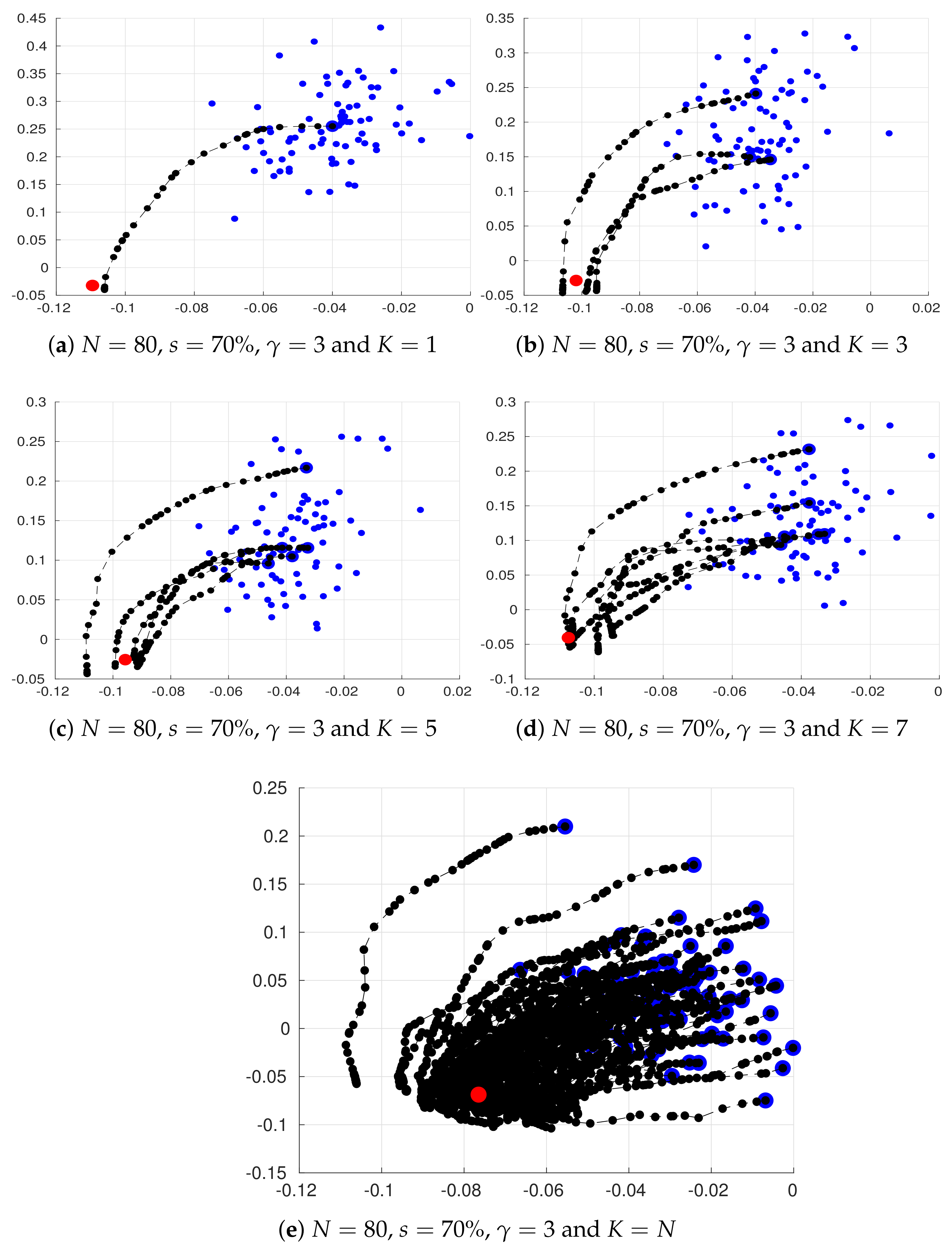
Yet another interesting analysis is the behaviour of the sampling process. In Figure 3, we show a two dimensional projection of our sampling steps for some particular choices of parameters , N, s, and K. We use the two leading components of the space generated by the accepted samples among iterations. Note that, in all cases, the sampling method obtains good estimates of the actual state of the system , even more, assuming (which is equivalent to assume Gaussian errors for each ensemble member), the sampling steps converges to .
5. Conclusions
In this paper we propose an EnKF implementation based on a modified Cholesky decomposition and a Markov-Chain-Monte-Carlo (MCMC) Method, the GMM-EnKF-MCMC. During the assimilation of observations, the method proceeds as follows: prior error distributions are fitted by using Gaussian Mixture Models. Prior components are estimated making use of the Expectation Maximization algorithm. Based on MCMC, posterior components are individually estimated. This is done by sampling states along an approximated steepest descent direction of the well-known Three Dimensional Variational cost function. Experimental tests are performed on the Lorenz-96 model. The results reveal that the proposed method is able to handle non-linearities produced by the model dynamics as well as those generated by the non-linear observation operator and even more, in a root-mean-square-error sense, the accuracy of the filter is not highly impacted as the degree of the observation operator is increased.
Acknowledgments
This work was supported by the Applied Math and Computer Science Laboratory at Universidad del Norte, Barranquilla, COL.
Author Contributions
Elias D. Nino-Ruiz and Haiyan Cheng conceived and designed the experiments; Elias D. Nino-Ruiz and Rolando Beltran performed the experiments; Elias D. Nino-Ruiz and Haiyan Cheng analyzed the data; Rolando Beltran contributed analysis tools; Elias D. Nino-Ruiz and Haiyan Cheng wrote the paper.
Conflicts of Interest
The authors declare no conflict of interest.
References
- Hoar, T.; Anderson, J.; Collins, N.; Kershaw, H.; Hendricks, J.; Raeder, K.; Mizzi, A.; Barré, J.; Gaubert, B.; Madaus, L.; et al. DART: A Community Facility Providing State-Of-The-Art, Efficient Ensemble Data Assimilation for Large (Coupled) Geophysical Models; AGU: Washington, DC, USA, 2016. [Google Scholar]
- Clayton, A.; Lorenc, A.C.; Barker, D.M. Operational implementation of a hybrid ensemble/4D-Var global data assimilation system at the Met Office. Q. J. R. Meteorol. Soc. 2013, 139, 1445–1461. [Google Scholar] [CrossRef]
- Fairbairn, D.; Pring, S.; Lorenc, A.; Roulstone, I. A comparison of 4DVar with ensemble data assimilation methods. Q. J. R. Meteorol. Soc. 2014, 140, 281–294. [Google Scholar] [CrossRef]
- Reynolds, D. Gaussian mixture models. Encycl. Biom. 2015, 827–832. [Google Scholar] [CrossRef]
- Nguyen, T.M.; Wu, Q.J.; Zhang, H. Bounded generalized Gaussian mixture model. Pattern Recogn. 2014, 47, 3132–3142. [Google Scholar] [CrossRef]
- Witten, I.H.; Frank, E.; Hall, M.A.; Pal, C.J. Data Mining: Practical Machine Learning Tools and Techniques; Morgan Kaufmann: Burlington, MA, USA, 2016. [Google Scholar]
- Mandel, M.I.; Weiss, R.J.; Ellis, D.P. Model-based expectation-maximization source separation and localization. IEEE Trans. Audio Speech Lang. Proc. 2010, 18, 382–394. [Google Scholar] [CrossRef]
- Vila, J.P.; Schniter, P. Expectation-maximization Gaussian-mixture approximate message passing. IEEE Trans. Signal Process. 2013, 61, 4658–4672. [Google Scholar] [CrossRef]
- Dovera, L.; Della Rossa, E. Multimodal ensemble Kalman filtering using Gaussian mixture models. Comput. Geosci. 2011, 15, 307–323. [Google Scholar] [CrossRef]
- Evensen, G. Data Assimilation: The Ensemble Kalman Filter; Springer: Secaucus, NJ, USA, 2006. [Google Scholar]
- Evensen, G. The ensemble Kalman filter: Theoretical formulation and practical implementation. Ocean Dyn. 2003, 53, 343–367. [Google Scholar] [CrossRef]
- Greybush, S.J.; Kalnay, E.; Miyoshi, T.; Ide, K.; Hunt, B.R. Balance and ensemble Kalman filter localization techniques. Mon. Weather Rev. 2011, 139, 511–522. [Google Scholar] [CrossRef]
- Buehner, M. Evaluation of a Spatial/Spectral Covariance Localization Approach for Atmospheric Data Assimilation. Mon. Weather Rev. 2011, 140, 617–636. [Google Scholar] [CrossRef]
- Anderson, J.L. Localization and Sampling Error Correction in Ensemble Kalman Filter Data Assimilation. Mon. Weather Rev. 2012, 140, 2359–2371. [Google Scholar] [CrossRef]
- Nino-Ruiz, E.D.; Sandu, A. Efficient parallel implementation of DDDAS inference using an ensemble Kalman filter with shrinkage covariance matrix estimation. Clust. Comput. 2017, 1–11. [Google Scholar] [CrossRef]
- Nino-Ruiz, E.D.; Sandu, A.; Deng, X. A parallel implementation of the ensemble Kalman filter based on modified Cholesky decomposition. J. Comput. Sci. 2017, in press. [Google Scholar] [CrossRef]
- Bickel, P.J.; Levina, E. Regularized estimation of large covariance matrices. Ann. Statist. 2008, 36, 199–227. [Google Scholar] [CrossRef]
- Nino-Ruiz, E.D.; Mancilla, A.; Calabria, J.C. A Posterior Ensemble Kalman Filter Based on A Modified Cholesky Decomposition. Procedia Comput. Sci. 2017, 108, 2049–2058. [Google Scholar] [CrossRef]
- Nino-Ruiz, E.D. A Matrix-Free Posterior Ensemble Kalman Filter Implementation Based on a Modified Cholesky Decomposition. Atmosphere 2017, 8, 125. [Google Scholar] [CrossRef]
- Attia, A.; Sandu, A. A hybrid Monte Carlo sampling filter for non-gaussian data assimilation. AIMS Geosci. 2015, 1, 41–78. [Google Scholar] [CrossRef]
- Attia, A.; Moosavi, A.; Sandu, A. Cluster Sampling Filters for Non-Gaussian Data Assimilation. arXiv, 2016; arXiv:1607.03592. [Google Scholar]
- Kotecha, J.H.; Djuric, P.M. Gaussian sum particle filtering. IEEE Trans. Signal Process. 2003, 51, 2602–2612. [Google Scholar] [CrossRef]
- Rings, J.; Vrugt, J.A.; Schoups, G.; Huisman, J.A.; Vereecken, H. Bayesian model averaging using particle filtering and Gaussian mixture modeling: Theory, concepts, and simulation experiments. Water Resour. Res. 2012, 48. [Google Scholar] [CrossRef]
- Moon, T.K. The expectation-maximization algorithm. IEEE Signal Process. Mag. 1996, 13, 47–60. [Google Scholar] [CrossRef]
- Alspach, D.; Sorenson, H. Nonlinear Bayesian estimation using Gaussian sum approximations. IEEE Trans. Autom. Control 1972, 17, 439–448. [Google Scholar] [CrossRef]
- Frei, M.; Künsch, H.R. Mixture ensemble Kalman filters. Comput. Stat. Data Anal. 2013, 58, 127–138. [Google Scholar] [CrossRef]
- Tagade, P.; Seybold, H.; Ravela, S. Mixture Ensembles for Data Assimilation in Dynamic Data-driven Environmental Systems1. Procedia Comput. Sci. 2014, 29, 1266–1276. [Google Scholar] [CrossRef]
- Sondergaard, T.; Lermusiaux, P.F. Data assimilation with Gaussian mixture models using the dynamically orthogonal field equations. Part I: Theory and scheme. Mon. Weather Rev. 2013, 141, 1737–1760. [Google Scholar] [CrossRef]
- Smith, K.W. Cluster ensemble Kalman filter. Tellus A 2007, 59, 749–757. [Google Scholar] [CrossRef]
- Hansen, P.R. A Winner’s Curse for Econometric Models: On the Joint Distribution of In-Sample Fit and Out-Of-Sample Fit and Its Implications for Model Selection; Research Paper; Stanford University: Stanford, CA, USA, 2010; pp. 1–39. [Google Scholar]
- Vrieze, S.I. Model selection and psychological theory: A discussion of the differences between the Akaike information criterion (AIC) and the Bayesian information criterion (BIC). Psychol. Methods 2012, 17, 228. [Google Scholar] [CrossRef] [PubMed]
- Van Leeuwen, P.J.; Cheng, Y.; Reich, S. Nonlinear Data Assimilation; Springer: Cham, Switzerland, 2015; Volume 2. [Google Scholar]
- Bannister, R. A review of operational methods of variational and ensemble-variational data assimilation. Q. J. R. Meteorol. Soc. 2017, 143, 607–633. [Google Scholar] [CrossRef]
- Snyder, C.; Bengtsson, T.; Bickel, P.; Anderson, J. Obstacles to high-dimensional particle filtering. Mon. Weather Rev. 2008, 136, 4629–4640. [Google Scholar] [CrossRef]
- Rebeschini, P.; Van Handel, R. Can local particle filters beat the curse of dimensionality? Ann. Appl. Probab. 2015, 25, 2809–2866. [Google Scholar] [CrossRef]
- Moré, J.J.; Sorensen, D.C. Computing a trust region step. SIAM J. Sci. Stat. Comput. 1983, 4, 553–572. [Google Scholar] [CrossRef]
- Conn, A.R.; Gould, N.I.; Toint, P.L. Trust Region Methods; SIAM: Philadelphia, PA, USA, 2000; Volume 1. [Google Scholar]
- Nino-Ruiz, E.D. Implicit Surrogate Models for Trust Region Based Methods. J. Comput. Sci. 2018, in press. [Google Scholar] [CrossRef]
- Wächter, A.; Biegler, L.T. On the implementation of an interior-point filter line-search algorithm for large-scale nonlinear programming. Math. Program. 2006, 106, 25–57. [Google Scholar] [CrossRef]
- Grippo, L.; Lampariello, F.; Lucidi, S. A nonmonotone line search technique for Newton’s method. SIAM J. Numer. Anal. 1986, 23, 707–716. [Google Scholar] [CrossRef]
- Kramer, O.; Ciaurri, D.E.; Koziel, S. Derivative-free optimization. In Computational Optimization, Methods and Algorithms; Springer: Berlin/Heidelberg, Germany, 2011; pp. 61–83. [Google Scholar]
- Conn, A.R.; Scheinberg, K.; Vicente, L.N. Introduction to Derivative-Free Optimization; SIAM: Philadelphia, PA, USA, 2009; Volume 8. [Google Scholar]
- Rios, L.M.; Sahinidis, N.V. Derivative-free optimization: A review of algorithms and comparison of software implementations. J. Glob. Optim. 2013, 56, 1247–1293. [Google Scholar] [CrossRef]
- Jang, J.S.R. Derivative-Free Optimization. In Neuro-Fuzzy Soft Computing; Prentice Hall: Englewood Cliffs, NJ, USA, 1997; pp. 173–196. [Google Scholar]
- Nino-Ruiz, E.D.; Ardila, C.; Capacho, R. Local search methods for the solution of implicit inverse problems. In Soft Computing; Springer: Berlin/Heidelberg, Germany, 2017; pp. 1–14. [Google Scholar]
- Anderson, J.L.; Anderson, S.L. A Monte Carlo implementation of the nonlinear filtering problem to produce ensemble assimilations and forecasts. Mon. Weather Rev. 1999, 127, 2741–2758. [Google Scholar] [CrossRef]
- Grubmüller, H.; Heller, H.; Windemuth, A.; Schulten, K. Generalized Verlet algorithm for efficient molecular dynamics simulations with long-range interactions. Mol. Simul. 1991, 6, 121–142. [Google Scholar] [CrossRef]
- Van Gunsteren, W.F.; Berendsen, H. A leap-frog algorithm for stochastic dynamics. Mol. Simul. 1988, 1, 173–185. [Google Scholar] [CrossRef]
- Koontz, W.L.; Fukunaga, K. A nonparametric valley-seeking technique for cluster analysis. IEEE Trans. Comput. 1972, 100, 171–178. [Google Scholar] [CrossRef]
- Lorenz, E.N. Designing Chaotic Models. J. Atmos. Sci. 2005, 62, 1574–1587. [Google Scholar] [CrossRef]
- Fertig, E.J.; Harlim, J.; Hunt, B.R. A comparative study of 4D-VAR and a 4D ensemble Kalman filter: Perfect model simulations with Lorenz-96. Tellus A 2007, 59, 96–100. [Google Scholar] [CrossRef]
- Karimi, A.; Paul, M.R. Extensive chaos in the Lorenz-96 model. Chaos 2010, 20, 043105. [Google Scholar] [CrossRef] [PubMed]
- Gottwald, G.A.; Melbourne, I. Testing for chaos in deterministic systems with noise. Physica D 2005, 212, 100–110. [Google Scholar] [CrossRef]
Figure 1.
Experimental results with the Lorenz-96 model (29). The time evolution of mean analysis errors and their standard deviation across the 10 different experimental configurations are reported for , and .
Figure 1.
Experimental results with the Lorenz-96 model (29). The time evolution of mean analysis errors and their standard deviation across the 10 different experimental configurations are reported for , and .
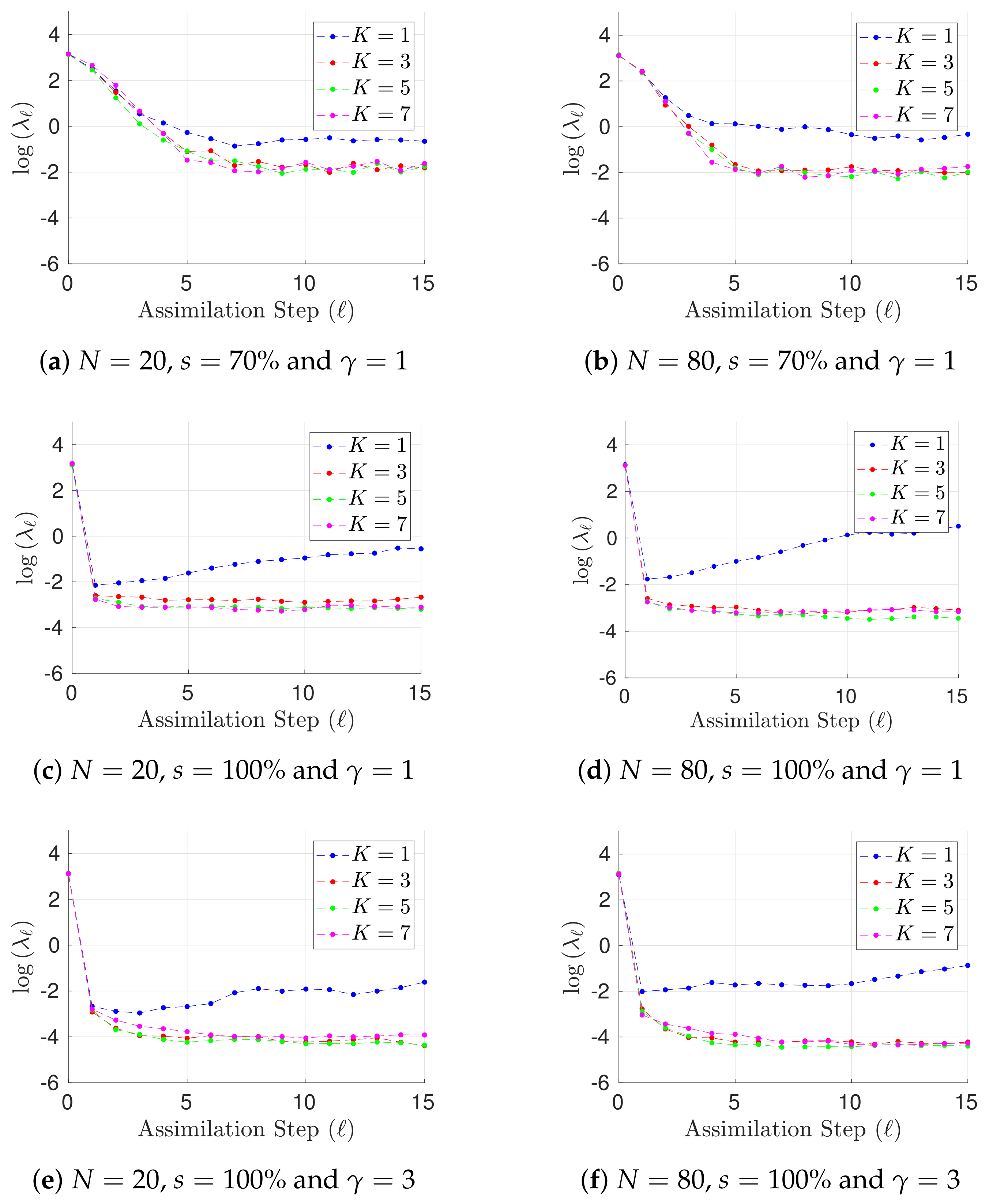
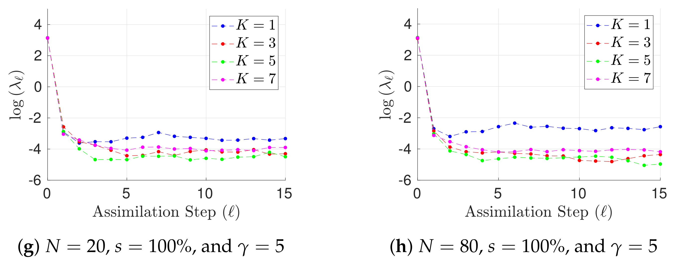
Figure 2.
Experimental results with the Lorenz-96 model (29). The time evolution of mean analysis errors and their standard deviation across the 10 different experimental configurations are reported for , and .
Figure 2.
Experimental results with the Lorenz-96 model (29). The time evolution of mean analysis errors and their standard deviation across the 10 different experimental configurations are reported for , and .
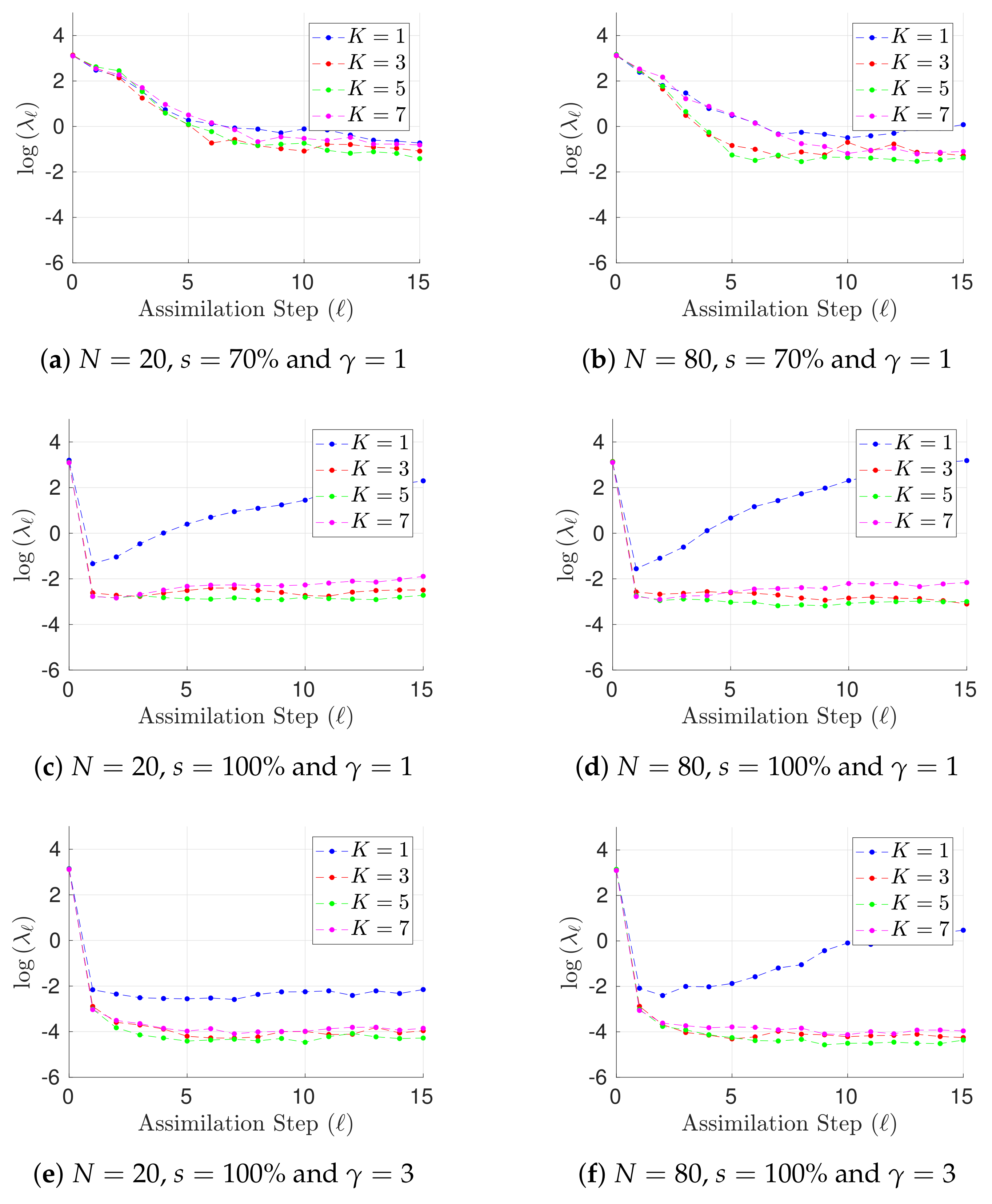
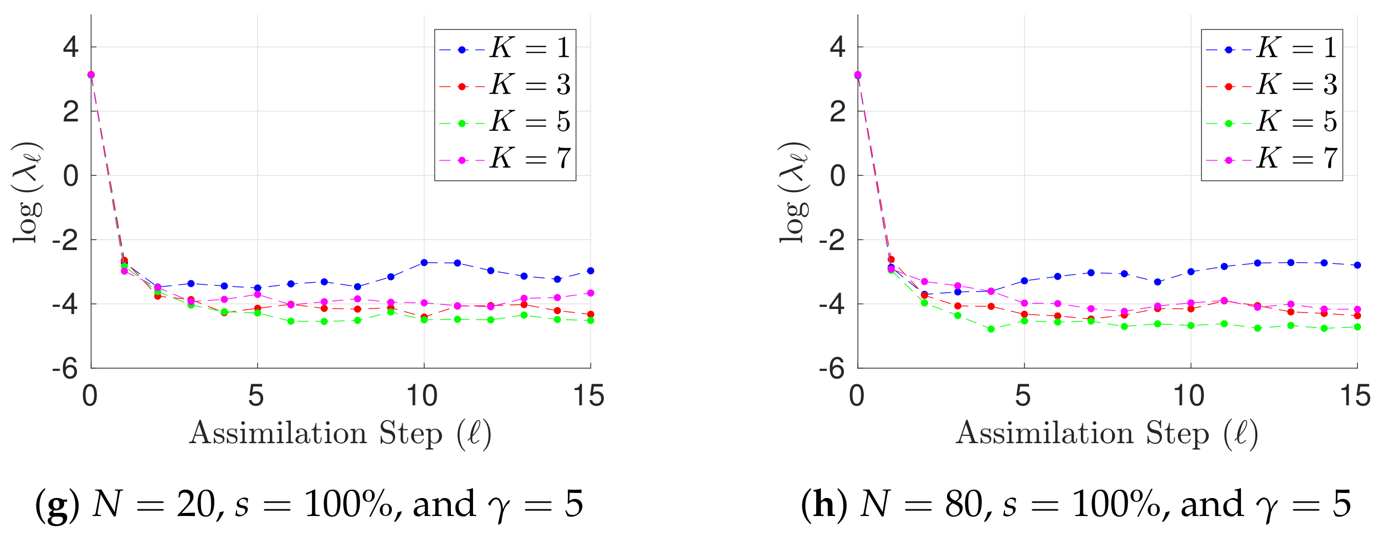
Figure 3.
Two dimensional projections of the steps performed by the sampling method. Blue dots denote prior ensemble members , large blue dots stand for centroids , dashed black lines together with black dots denote accepted states , and the red dot stands for the actual state of the system . Even for , the method is able to obtain reasonable estimates of the actual state of the system. The variance explained in such plots is larger than .


Table 1.
Experimental results with the Lorenz-96 model. Mean of RMSE values are reported across the 10 different experimental configurations for different configuration of parameters , s, K, and . The number of ensemble members equals .
Table 1.
Experimental results with the Lorenz-96 model. Mean of RMSE values are reported across the 10 different experimental configurations for different configuration of parameters , s, K, and . The number of ensemble members equals .
| 70% | 16 h |  |  |  |
| 50 h |  |  |  | |
| 100% | 16 h |  |  |  |
| 50 h |  |  |  |
Table 2.
Experimental results with the Lorenz-96 model. Mean of RMSE values are reported across the 10 different experimental configurations for different configuration of parameters , s, K, and . The number of ensemble members equals .
Table 2.
Experimental results with the Lorenz-96 model. Mean of RMSE values are reported across the 10 different experimental configurations for different configuration of parameters , s, K, and . The number of ensemble members equals .
| s | ||||
|---|---|---|---|---|
| 70% | 16 h |  |  |  |
| 50 h |  |  |  | |
| 100% | 16 h |  |  |  |
| 50 h |  |  |  |
© 2018 by the authors. Licensee MDPI, Basel, Switzerland. This article is an open access article distributed under the terms and conditions of the Creative Commons Attribution (CC BY) license (http://creativecommons.org/licenses/by/4.0/).
Share and Cite
MDPI and ACS Style
Nino-Ruiz, E.D.; Cheng, H.; Beltran, R. A Robust Non-Gaussian Data Assimilation Method for Highly Non-Linear Models. Atmosphere 2018, 9, 126. https://doi.org/10.3390/atmos9040126
AMA Style
Nino-Ruiz ED, Cheng H, Beltran R. A Robust Non-Gaussian Data Assimilation Method for Highly Non-Linear Models. Atmosphere. 2018; 9(4):126. https://doi.org/10.3390/atmos9040126
Chicago/Turabian StyleNino-Ruiz, Elias D., Haiyan Cheng, and Rolando Beltran. 2018. "A Robust Non-Gaussian Data Assimilation Method for Highly Non-Linear Models" Atmosphere 9, no. 4: 126. https://doi.org/10.3390/atmos9040126
Note that from the first issue of 2016, this journal uses article numbers instead of page numbers. See further details here.