Article

Sensitive versus Rough Dependence under Initial Conditions in Atmospheric Flow Regimes

1
Department of Soil, Environmental, and Atmospheric Sciences, University of Missouri, Columbia, MO 65211, USA
2
Department of Mathematics, University of Missouri, Columbia, MO 65211, USA
3
Department of Mechanical and Aerospace Engineering, University of Missouri, Columbia, MO 65211, USA
*
Author to whom correspondence should be addressed.
Atmosphere 2016, 7(12), 157; https://doi.org/10.3390/atmos7120157
Submission received: 5 October 2016 / Revised: 28 November 2016 / Accepted: 30 November 2016 / Published: 5 December 2016

Abstract

:
In this work, we will identify the existence of “rough dependence on initial conditions” in atmospheric phenomena, a concept which is a problem for weather analysis and forecasting. Typically, two initially similar atmospheric states will diverge slowly over time such that forecasting the weather using the Navier-Stokes equations is useless after some characteristic time scale. With rough dependence, two initial states diverge very quickly, implying forecasting may be impossible. Using previous research in atmospheric science, rough dependence is characterized by using quantities that can be calculated using atmospheric data and quantities. Rough dependence will be tested for and identified in atmospheric phenomena at different time scales using case studies. Data were provided for this project by archives outside the University of Missouri (MU) and by using the MU RADAR at the South Farm experiment station.

1. Introduction

In atmospheric sciences, weather forecasters today rely on numerical models in order to make predictions (synoptic-scale), and these can be made reliably out to about seven days, sometimes quite well (e.g., Winter Storm Jonas 22–23 January 2016—impacted the Eastern USA) but the absolute limit is about 10–14 days. However, numerical weather forecasts at the same time and spatial scale can fail in the one-to-two-day time frame, or even more quickly (e.g., Tropical Cyclone Patricia 22–23 October 2015—Eastern Pacific Ocean basin). The general reasons for their failure is threefold, and these are (a) incomplete knowledge of physical processes (parameterization—e.g., latent heat); (b) lack of data, and (c) measurement error (e.g., [1,2]). Then, error in the initial and/or boundary conditions can yield model forecasts as quickly as a few days [3], and this behavior, which is inherent in the Navier Stokes equations, is called sensitive dependence on the initial conditions (SDOIC) [4]. At smaller scales, predictability has improved greatly in the last 20 years, which has saved lives and property. However, smaller-scale systems can also change radically over very small time scales (e.g., 5–10 min) as detected by RADAR.
One way that the forecasting community can mitigate or qualitatively represent SDOIC in weather forecast model output is through the use of ensemble modeling techniques (e.g., [5,6,7]), and an example of these kinds of operational products can be found at [8] Ensemble modeling techniques were produced at the National Centers for Environmental Prediction (NCEP), and have been in use for more than two decades [7]. The NCEP forecasts are produced using 17 different runs of the global model using the initial conditions, and these are assumed to be within the range of analysis error. Then, the ensemble mean performs typically better than any of the individual runs. The most widely used ensemble products choose representative contours of 500 hPa, and a plot of all these realizations on a map. These are called “spaghetti plots”, since the contours will look like a plate of spaghetti after some period of time when the forecasts diverge. Often, but not always, when the spread among the ensembles is small, forecasts are more skillful.
In the study of atmospheric phenomena, the behavior of geophysical fluids at different time and spatial scales using the Navier-Stokes equations is elucidated through the use of scaling parameters. For example, the assumption that the atmosphere is close to being geostrophically balanced can be represented using the Rossby Number (e.g., [9]), which is the ratio of the fluid acceleration (difference between pressure gradient force and Coriolis force) and the inertial (Coriolis) forces. If the Rossby Number is zero, the atmosphere is nearly geostrophically balanced, although this condition is an ideal condition that assumes the atmosphere is inviscid and in asteady state. However, there is always some departure from geostrophy in the observed atmosphere (e.g., [10]). The Reynolds number is the ratio between the inertial to viscous forces. If the Reynolds Number is large, the atmospheric flow is three-dimensional and is dominated by inertial forces. Such a flow possesses turbulence as represented by eddies and vortices. Low Reynolds Number flows are laminar (two dimensional), and viscous forcing is dominant.
Using the Reynolds Number, a characteristic growth rate for a disturbance in a flow can be derived. If the growth rate of an atmospheric disturbance is smaller than that implied by the characteristic time scale, then SDOIC will characterize the forecast of the system and these forecasts represented by trajectories (or contours in the “spaghetti plots”) will diverge slowly with time. If the growth rate is greater than that implied by a characteristic time scale, then trajectories will diverge exponentially with time. This indicates that predictability may not be possible. In this case, the flow is roughly dependent on the initial conditions (RDOIC) [11,12]. After the characteristic time-scale, the amplification of the individual atmospheric disturbance is characterized by an exponential function of time with growth rate independent of the Reynolds Number [11], i.e., sensitive dependence on initial conditions (SDOIC). When the Reynolds Number is large, the first stage amplification is dramatic and long lasting. Since atmospheric disturbances are ubiquitous, the second stage amplification plays a very minor role in the evolution of fully developed turbulence. SDOIC implies that long-term predictability is not possible (short-term predictability is still possible), while RDOIC implies short-term predictability is not possible.
Rough dependence on initial conditions is a new theory about the nature of turbulence in fluid flows [11,12] under the conditions of a large Reynolds Number. Fluid dynamics have long suspected that turbulence is more than just a chaotic flow. Like SDOIC, RDOIC can occur in an ensemble where the initial conditions of each member are very similar, except that where in SDOIC their divergence occurs slowly with time, in RDOIC, the trajectories diverge very rapidly [11]. This theory also states that in high Reynolds Number flows, RDOIC represents “violent” turbulence [11]. In a meteorological context, unpredictable and rapidly growing phenomena are said to undergo “explosive” development (e.g., [13]). For the Navier-Stokes equations under a periodic boundary condition, RDOIC has been verified numerically [14]. However, there is no discussion as of yet of RDOIC in the atmospheric science literature. Thus, the goal of this work is to demonstrate the existence of RDOIC in examples of both large- and smaller-scale atmospheric phenomena, and differentiate this from SDOIC. In accomplishing this task, we will develop methods for quantifying this in atmospheric flows in Section 2. Case studies will be presented in Section 3, and a summary and conclusions will be presented in Section 4.

2. Experiments

2.1. Data

In order to meet our objectives, several data sets will be used. The first is the National Centers for Environmental Prediction/National Center for Atmospheric Research (NCEP/NCAR) re-analyses, archived at the NCAR research facilities in Boulder, CO (e.g., [15,16]), which can be used to provide large-scale meteorological data at various resolutions from 1° × 1° to 2.5° × 2.5° latitude-longitude grids. Then, the tropical cyclone occurrence, intensity, and central pressure data for all ocean basins were downloaded via the UNISYS website [17].
RADAR data archived at the University of Missouri RADAR located at the South Farm research station will also be utilized. These data are readily available from the RADAR Applications, Instrumentation, And Nowcasting Systems (RAINS) laboratory participating in the Experimental Program to Stimulate Competitive Research (EPSCoR) project, which is available in decibel levels (dBZ). Here, we will identify coherent features as those at 30 dBZ or more.
The RADAR data used in this work were acquired by the MZZU X-band dual-polarization radar located at 38.906° N, 92.269° W. The RADAR has a beam width of 1.27 degrees and operates with a gate length of 260 m, with an unambiguous radial velocity range of ±22.5 m/s. The radial velocity data is dealiased, and the azimuthal shear field is derived using the two-dimensional local, linear least squares derivative (LLSD) methodology described in [18] and implemented in the Warning Decision Support System-Integrated Information (WDSS-II: [19]) using a 750 m by 1500 m kernel. The native reflectivity and azimuthal shear fields are then converted to a Cartesian grid using the data merger package of [20], resulting in a 0.5 km grid of azimuthal shear values.
Areas of precipitation are identified as areas of contiguous pixels of reflectivity above a specified threshold (30 dDZ), and the azimuthal shear values from these areas are extracted, as described in [20]. In this case, a reflectivity threshold of 10 dBZ was chosen in order for convective cells in the early growth stage to be observed and tracked through their development phase. Association of cells from one radar scan to the next was achieved manually in this case by comparison of storm centroid location at consecutive time steps and examination of the imagery.

2.2. Methods

SDOIC occurs in a system where at least one Lyapunov Exponent is positive, and as stated above is a measure of divergence for the trajectories of two systems that are initially close. SDOIC also demonstrates the presence of chaos. The Lyapunov Exponent is defined as the characteristic exponent in the solution of a differential equation and is expressed as:
λ i = lim t { lim ε ( 0 ) 0 [ 1 t ] ln ( ε i ( t ) ε ( 0 ) ) } ,   i = 1 , n
where λi is the ith Lyapunov Exponent of an n-dimensional system. The notations ε(0) and ε(t) represent the initial and final state, respectively, of a quantity for which a differential equation is solved. With respect to the atmosphere, [21] postulated that if the atmosphere is barotropic, the positive Lyapunov Exponent in the atmosphere can be expressed as the area integrated regional enstrophy (IRE):
i > 0 λ i A ς 2 d A
where ζ is the vorticity (s−1), or the curl of the wind vector. This quantity squared is called enstrophy (s−2), which is defined as the dissipation tendency of a fluid (e.g., [22]). It should be noted that [21] found a high correlation between the Lyapunov exponent and the IRE. The dimensions on each side of (2) are not identical, and in theory, there is a constant of proportionality between them whose value is close to unity. The work of [23] (and references therein) demonstrated the utility of this quantity in identifying the onset and termination of atmospheric blocking and flow regime transformation. The calculations for IRE were made using the 500 hPa wind fields using the methodology of [23] for the blocking event and the hurricane, and using the RADAR-derived values for vorticity and shear for the case of convection.
As a positive Lyapunov Exponent, this quantity relates to predictability and can also be related to Kolmogorov Entropy (or metric entropy) (e.g., [24]). The larger the IRE, the less predictable the atmosphere, as trajectories of two initial conditions would diverge rapidly.
In [11], RDOIC is defined using Equation (1) and representing short term rapid growth as (using the notation of Equation (1)—in [11], the variable used was “u” or fluid flow; here, we just use x for any quantity):
λ r = lim t 0 + 1 t α ln ( x ( t ) x ( 0 ) )
where the Lyapunov Exponent represents rapid growth over a short time, under the condition that the exponent α > 0. Then [11], applied this principle in the Navier-Stokes equation in order to estimate the temporal growth of modes in the equation, and the result is (for more detail, see [11]);
x ( t ) e C t   Re + C 1 t ( x ( o ) )
where Re is the Reynolds Number as defined in Section 1, t is time and C and C1 are defined below. Thus, this implies exponential growth with the square root of time and the Reynolds Number that is larger than that implied by the Lyapunov Exponent, or violent turbulence is RDOIC. Then, using Equation (2) and substituting into Equation (3) for the Lyapunov Exponent, and comparing to Equation (4), we can define RDOIC in terms of quantities that can be measured and then calculated directly from an atmospheric flow. RDOIC can be estimated as:
A ζ 2 d A C t   Re + C 1 t
a newly derived expression that can be used to evaluate the presence of RDOIC versus SDOIC in terms of atmospheric phenomena. In Equation (5) above, the constants C and C1 are (see [11]):
C = 8 2 e m a x τ [ 0 , T ]   | | u ( τ ) | | n
C 1 = 2 e 2 C
where C1 is written in terms of C, and C is a function of the maximum fluid velocity (m·s−1) in the time domain (τ) examined.
In Equation (5) above, vorticity (ζ) can be calculated by taking the curl of the wind vector, or vorticity can be defined as circulation per unit area;
ζ ( v x u y ) lim Δ A 0 ( Δ C Δ A )
where ΔC is some change in circulation and ΔA—the change in area, and in Equation (7), we can estimate ΔC as;
C V d r V h Δ r Δ C
where V is the velocity vector, and r—the position vector.

3. Results

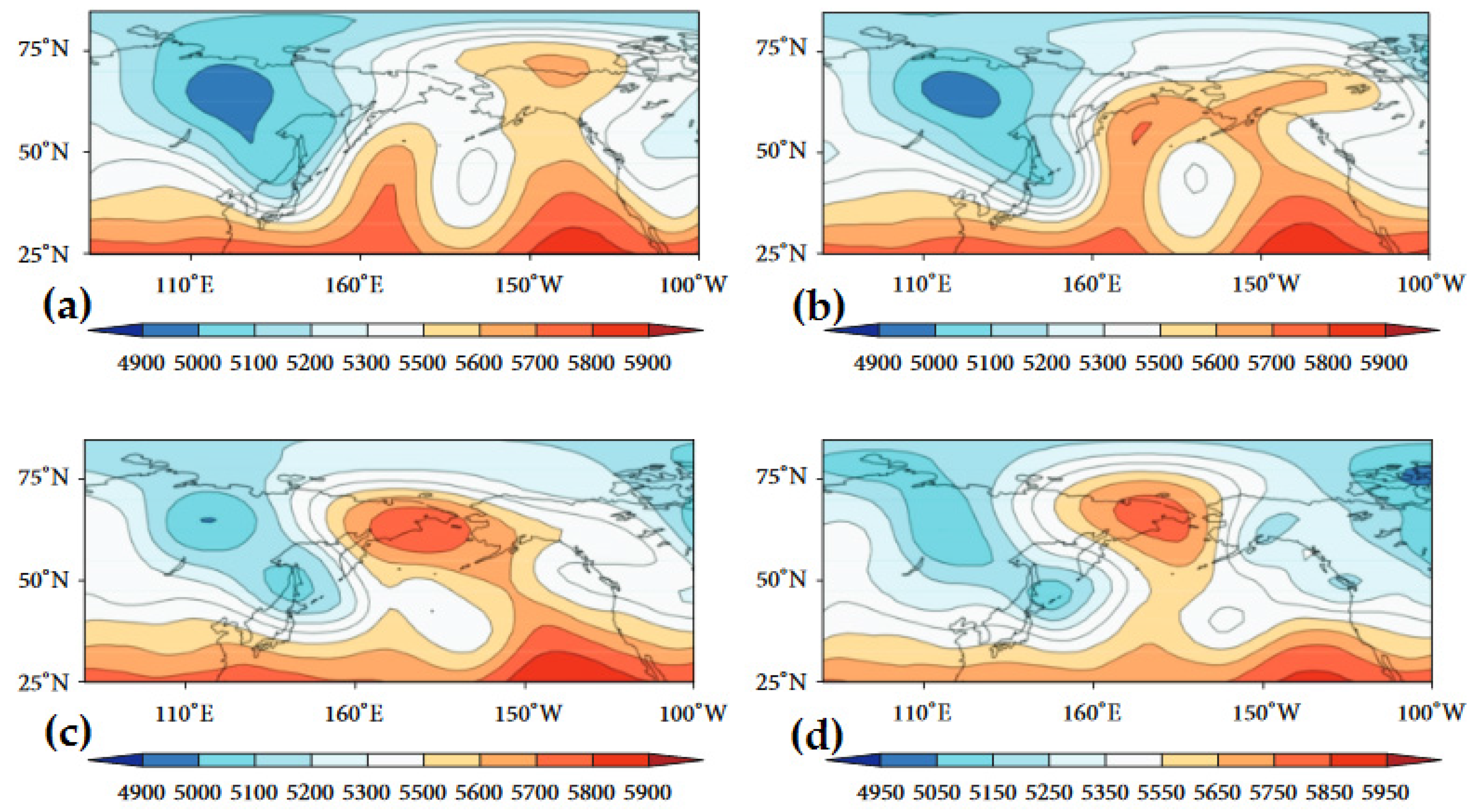
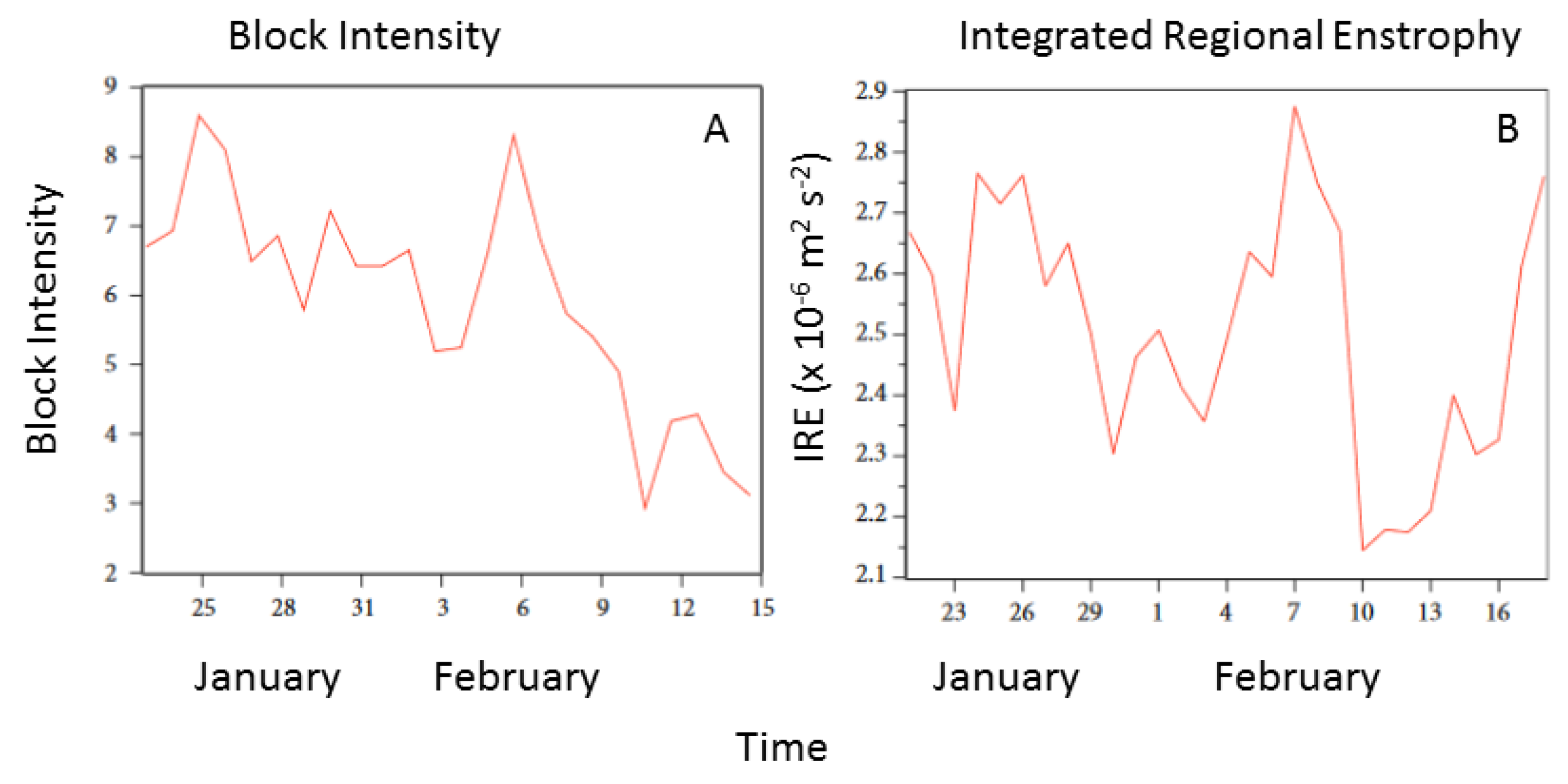
3.1. Case Study, Atmospheric Blocking

The blocking event examined here occurred from 23 January to 16 February 2014 and was located over the Eastern Pacific near the Gulf of Alaska and near the West Coast of North America (130° W) (see the University of Missouri blocking archive [25]). This event formed out of a very long-lived ridge over the same area. The event dominated a significant period of the winter season and was likely responsible for the cold winter over North America that year (e.g., [26]). The work of [27] describes this event in more detail and the 500 hPa heights during the intensification stage of the blocking event, which is shown in Figure 1. This event was noteworthy as it survived a large-scale flow regime change during early 4–7 February 2014, as the Pacific North American (PNA) teleconnection pattern changed from a positive to negative configuration during early February 2014. Earlier work (e.g., [28,29]) suggested that blocking events should not survive a transition in the large-scale flow regime, but [27] showed that, under certain conditions, these events could survive the transition. Additionally, this event is noteworthy for its longevity and persistence.
Examining the block intensity (BI) [30] for this case (Figure 2a) demonstrated that the block was more intense just following the onset of the event, and then intensified in early February close to the same time that the phase of the PNA changed from positive to negative, indicating a flow regime transition. Then, BI was markedly lower, indicating a weaker block until the decay period. The IRE diagnostic also followed a similar evolution during the block lifecycle (Figure 2b), with the IRE maximized during onset, intensification, and termination. Then a calculation using Equation (5) demonstrates that for this blocking event (which is relatively large-scale), the evolution is dominated by quasi-geostropic processes (e.g., [9,10]) and SDOIC dynamics. The values shown in Table 1 using the IRE over the Northern Hemisphere are larger but of similar magnitude to those calculated using the Reynolds Number on the right-hand-side (RHS) of Equation (5). Also note that the vorticity is about the same magnitude as that for a hurricane event described below. Recall that [11] argued that RDOIC would exist if the time scale for the growth and evolution of a system is smaller than that implied by the Reynolds Number. For a typical synoptic-scale flow field (length-scale—5000 km, time-scale—105 s), the Reynolds Number is estimated to be about 2.3 × 10⁸, which was calculated using a script called Standard Atmosphere Computations [31]. Blocking events can be characterized as a similar scale phenomenon.

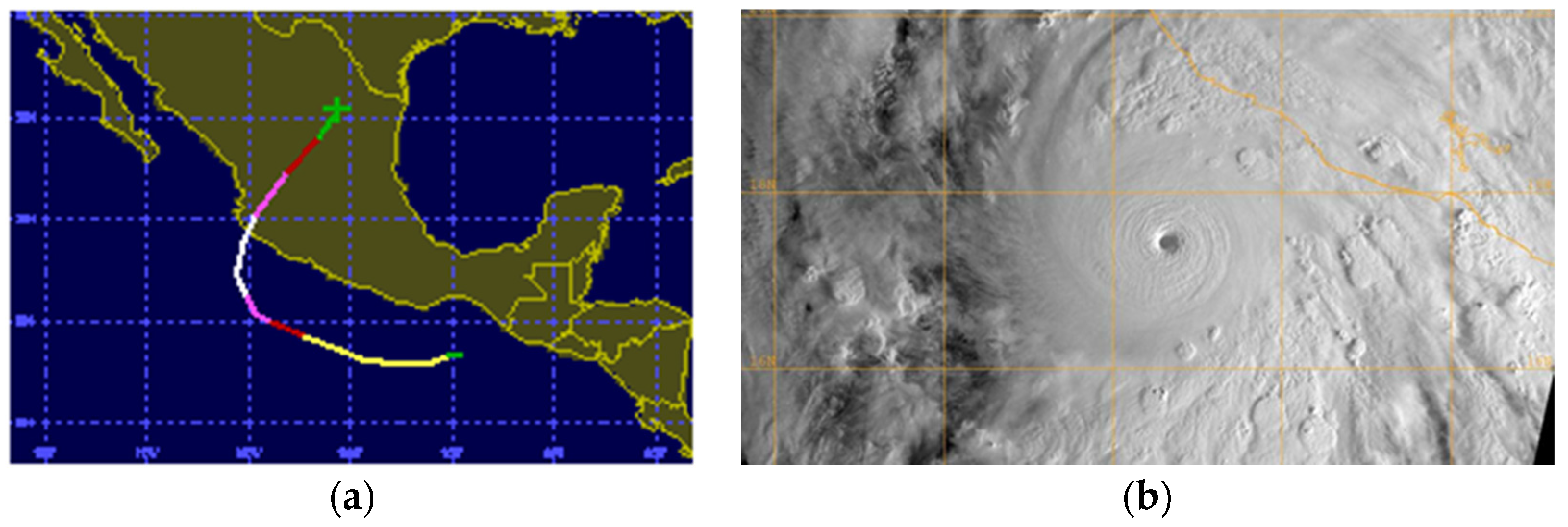
3.2. Case Study, Hurricane Patricia

Hurricane Patricia was an intense eastern Pacific tropical cyclone that occurred in late October 2015 and moved inland over western Mexico as a Category 5 event using the Saffir-Simpson Scale (Figure 3). This hurricane formed out of a tropical depression over the southeastern Pacific Ocean Basin [32] and was classified as a tropical storm early (0300 UTC) on 21 October 2015, with a central pressure of 1004 hPa. Patricia became a hurricane approximately 30 h later, and reached maximum intensity (about 100 m·s−1) 24 h after becoming a hurricane with a central pressure of 880 hPa, making it the most intense storm over the period of record (since 1970) by that measure in the eastern Pacific Ocean Basin. The total pressure fall was 124 hPa in 42 h (3.0 hPa·h−1), which given the low-latitude (~20° N), is nearly 7.5 times the rate for the definition of explosive cyclogenesis published by [33] and called the “bomb” rate. Most of the pressure fall (100 hPa) occurred during a 24 h period from 0900 UTC 22 October to 0900 UTC 23 October 2015, and this rate is more than 10 times the bomb rate.
The development rate of Hurricane Patricia was more consistent with that of mesoscale phenomena, and the development of tropical cyclones is recognized to be comprised of several mesoscale convective systems (MCVs) (e.g., [34]). Additionally, intense tropical cyclone environments cannot reasonably be described as geostrophic. The eyewall is frequently non-hydrostatic, and models of these environments use gradient wind approximations (e.g., [35]). Calculations using Equation (5) were carried out by considering Hurricane Patricia as a synoptic-scale entity (length and time scales as in Section 3.1) in a synoptic-scale environment (Table 1). The vorticity value is consistent with that of the blocking event environment. The IRE diagnostic term in this case is about an order of magnitude smaller than the RHS, indicating RDOIC dynamics or violent turbulence [11] is likely present. If Hurricane Patricia was considered a mesoscale feature (length scale—500 km time scale—104 s) in a mesoscale environment, the IRE diagnostic is more than an order of magnitude larger than the RHS (not shown) as the IRE diagnostic would be at least partly scale-dependent.
Hurricane track prediction has substantially improved in recent years, and the model forecasts issued near the time for the commencement of rapid deepening for the track of Patricia performed very well (Figure 4). At this time, Patricia was classified as a tropical storm. The intensity of Patricia was not well forecasted, however, as the suite of models forecast maximum intensity to occur 36 h later, with maximum winds at just more than half (50–55 m·s−1 versus 100 m·s−1) and a central pressure much higher (950–960 hPa versus 880 hPa) than observed. Thus, even with rapid deepening about to commence, the suite of models that are tuned specifically for hurricane forecasting (e.g., the Hurricane Weather Research Forecast (HWRF) model) failed to capture the intensity. This forecast represents a dramatic example of the problems inherent in forecasting smaller-scale events.

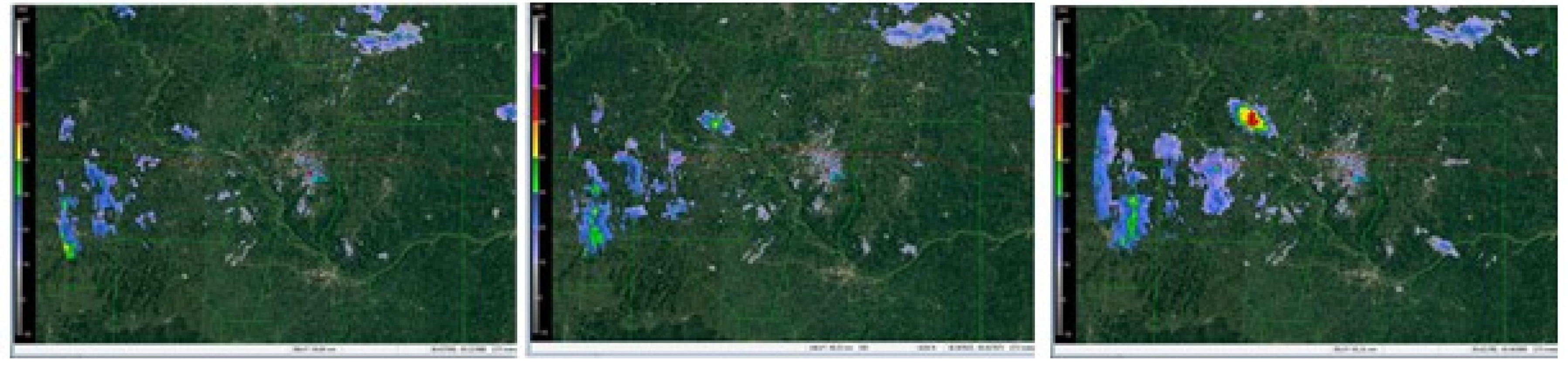
3.3. Case Study—Midwest Rain Event

At 1200 UTC 18 September 2015, a cold front stretched from Hudson Bay down through the central USA, terminating near the west coast (Figure 5). A local area of low pressure located on the front, which was identified near the borders of Missouri, Illinois, and Iowa. The cold front was located across northern Missouri at this time. Convection associated with this system began at approximately 1511 UTC and developed rapidly from this time to about 1543 UTC. The sequence of rapid development is illustrated in the RADAR images (Figure 6), which show convection 1516 and 1521 UTC. There were several cells identified at the initial time and tracked throughout the time period, and cell number 51 showed the maximum development rate as represented by the change in the number of pixels, which was 25 in scan four to 3695 in scan five.
In order to estimate the terms in Equation (5), the convection was considered a small-scale phenomenon in a mesoscale environment (500 km), and calculating the Reynolds number resulted in a value similar to those in the previous two case studies and similar values for the RHS of Equation (5). In order to estimate the IRE diagnostic, the maximum and minimum azimuthal shear (AZ) values were used in Table 1 rather than vorticity in order to estimate the largest possible value for IRE associated with this small-scale event. These are associated with the convection itself and have the same unit as vorticity. There were seven data slices (scans) available in the 32-min time period. As it was difficult to choose one particular entity to track, the maximum IRE for each of the seven time periods were used. The maximum IRE values ranged between 0.52 × 10⁷ m2·s2 (second scan) and 3.59 × 10⁷ m2·s2 (sixth scan—also Table 1). These values are about one order of magnitude less than the right-hand side. Similar tests for calculating IRE using mean values of AZ yields values two orders of magnitude less than those cited above and in Table 1. Using RADAR estimated vorticity for the environment (maximum of 5.8 × 10⁻⁴) produces IRE values several orders of magnitude less than those in Table 1 even though the vorticity value given here is much larger than the value for the blocking or the hurricane environments. Thus, for localized convective development, the conditions for RDOIC dynamic development are present. We considered here the phenomena to be a mesoscale region of convection in a mesoscale environment (see Section 3.2).

4. Discussion and Conclusions

The objectives of this study were to determine whether RDOIC exists in observed atmospheric phenomena and to develop a relationship to diagnose RDOIC as a function of observable atmospheric quantities. This relationship was developed in Section 2. Then, using observed atmospheric data for a long-lived blocking event, Hurricane Patricia, and a Midwestern USA convective event, Equation (5) was used to determine whether these cases were governed by quasi-geostrophic and SDOIC or RDOIC dynamics. This strategy was used to test several temporal and spatial scale phenomena.
While blocking can develop very rapidly, and models fail to anticipate their onset and/or decay [37], the results here suggest that the long-lived, Pacific Region winter blocking event of 2014 was likely governed by quasi-geostrophic and SDOIC dynamics. The spatial and time scale for blocking in general is consistent with that of the synoptic and planetary scales. The results here suggest that predictability for this type of event is at least possible for a weather forecast model.
In the case of Hurricane Patricia, an extremely rapidly developing event, the numerical models failed to predict the intensity the storm would attain within 24 h of the onset of rapid deepening. The model forecasts were not aggressive or fast enough in predicting the storm’s final severity. Hurricane Patricia likely developed at a rate consistent with convective-scale phenomena (meso-β or γ), and the calculation using Equation (5) demonstrated the possible presence of RDOIC dynamics.
It could be argued that the excessive deepening of Hurricane Patricia occurred as the result of excessive latent heat release [34,35], which is not explicitly represented in simplified versions of the NS equations. Thus, it might be difficult to differentiate SDOIC and RDOIC here. The work of [12,14] extended that of [11] to include viscous effects and found solutions to the NS equations. Also, [10] showed that latent heat release feeds back on the ageostrophic component of motion in the atmosphere, and thus would be included in the observed velocity used in the calculations here.
Finally, a fall season convective event that occurred over the Midwest USA (18 September 2015) was studied using RADAR derived azimuthal shear and estimated vorticity in order to calculate IRE. Even though the estimated vorticity and AZ were very large compared to the blocking event and hurricane environment, the calculated IRE diagnostic is smaller for smaller-scale phenomena and the RHS of the inequality of Equation (5). As in the case of Hurricane Patricia, however, this mesoscale-γ event could have been associated with RDOIC dynamics.

Acknowledgments

The authors would like to thank the anonymous reviewers for their comments, which made this contribution stronger. This work was partially funded under the Missouri EPSCoR project supported by the National Science Foundation under Award Number IIA-1355406. Any opinions, findings, and conclusions or recommendations expressed in this material are those of the authors and do not necessarily reflect the views of the National Science Foundation.

Author Contributions

Y. Charles Li, Anthony R. Lupo, Neil I. Fox, and Z. C. Feng conceived and designed the experiments; Neil I. Fox, Michael J. Simpson, and Jordan L. Rabinowitz performed the experiments; all the co-authors analyzed the data; and Anthony R. Lupo, Neil I. Fox, and Y. Charles Li wrote the paper.

Conflicts of Interest

The authors declare no conflict of interest.

References

  1. Haltiner, G.J.; Williams, R.T. Numerical Prediction and Dynamic Meteorology, 2nd ed.; Wiley and Sons, Inc.: Hoboken, NJ, USA, 1980. [Google Scholar]
  2. Durran, D.R. Numerical Methods for Wave Equations in Geophysical Fluid Dynamics; Springer: Berlin, Germany, 1999. [Google Scholar]
  3. Lorenz, E.N. Deterministic, non-periodic flow. J. Atmos. Sci. 1965, 20, 130–141. [Google Scholar] [CrossRef]
  4. Lorenz, E.N. A study of the predictability of a 28-variable model. Tellus 1963, 17, 321–333. [Google Scholar] [CrossRef]
  5. Toth, Z.; Kalnay, E. Ensemble forecasting at NCEP: The generation of perturbations. Bull. Am. Meteorol. Soc. 1993, 74, 2317–2330. [Google Scholar] [CrossRef]
  6. Toth, Z.; Kalnay, E. Ensemble forecasting at NCEP and the breeding method. Mon. Weather Rev. 1997, 125, 3297–3319. [Google Scholar] [CrossRef]
  7. Tracton, M.S.; Kalnay, E. Operational ensemble forecasting at the National Meteorological Center: Practical Aspects. Weather Forecast. 1993, 8, 379–398. [Google Scholar] [CrossRef]
  8. National Centers for Environmental Prediction Ensemble Products. Available online: http://www.esrl.noaa.gov/psd/map/images/ens/ens.html#nh (accessed on 5 December 2016).
  9. Holton, J.R.; Hakim, G.J. An Introduction to Dynamic Meteorology; Academic Press, Elsevier: Amsterdam, The Netherlands, 2012. [Google Scholar]
  10. Lupo, A.R. The role of ageostrophic forcing in a Height Tendency Equation. Mon. Weather Rev. 2002, 130, 115–126. [Google Scholar] [CrossRef]
  11. Li, Y.C. The distinction of turbulence from chaos—Rough dependence on initial data. Electron. J. Differ. Equ. 2014, 2014, 1–8. [Google Scholar]
  12. Li, Y.C. Rough Dependence upon Initial Data Exemplified by Explicit Solutions and the Effect of Viscosity. Available online: https://arxiv.org/abs/1506.05498 (accessed on 1 December 2016).
  13. Lupo, A.R.; Smith, P.J.; Zwack, P. A diagnosis of the development of two extratropical cyclones. Mon. Weather Rev. 1992, 120, 1490–1523. [Google Scholar] [CrossRef]
  14. Feng, Z.C.; Li, Y.C. Short term unpredictability of high Reynolds number turbulence—Rough dependence on initial data. Unpublished work. 2016. [Google Scholar]
  15. Kalnay, E.; Kanamitsu, M.; Kistler, R. The NCEP/NCAR 40-year reanalysis project. Bull. Am. Meteorol. Soc. 1996, 77, 437–471. [Google Scholar] [CrossRef]
  16. Kistler, R.; Kalnay, E.; Collins, W. The NCEP-NCAR 50-year reanalysis: Monthly means CD-ROM and documentation. Bull. Am. Meteorol. Soc. 2001, 82, 247–267. [Google Scholar] [CrossRef]
  17. UNISYS Weather Website. Available online: http://weather.unisys.com (accessed on 5 December 2016).
  18. Smith, T.M.; Elmore, K.L. The use of radial velocity derivatives to diagnose rotation and divergence. In Proceedings of the 11th Conference on Aviation, Range, and Aerospace, Hyannis, MA, USA, 4–8 October 2004.
  19. Lakshmanan, V.; Smith, T.; Hondl, K.; Stumpf, G.; Witt, A. A Real-Time, Three-Dimensional, Rapidly Updating, Heterogeneous Radar Merger Technique for Reflectivity, Velocity, and Derived Products. Weather Forecast. 2006, 21, 802–823. [Google Scholar] [CrossRef]
  20. Lack, S.A.; Fox, N.I. Development of an automated approach for identifying convective storm type using reflectivity-derived and near-storm environment data. Atmos. Res. 2012, 116, 67–81. [Google Scholar] [CrossRef]
  21. Dymnikov, V.P.; Kazantsev, Y.V.; Kharin, V.V. Information entropy and local Lyapunov exponents of barotropic atmospheric circulation. Izv. Atmos. Ocean. Phys. 1992, 28, 425–432. [Google Scholar]
  22. Weiss, J. The dynamics of enstrophy transfer in two-dimensional hydrodynamics. Phys. D Nonlinear Phenom. 1991, 48, 273–294. [Google Scholar] [CrossRef]
  23. Jensen, A.D.; Lupo, A.R. Using enstrophy based diagnostics in an ensemble for two blocking events. Adv. Meteorol. 2013, 2013, 693859. [Google Scholar] [CrossRef]
  24. Ott, E. Chaos in Dynamical Systems; Cambridge University Press: New York, NY, USA, 1993. [Google Scholar]
  25. University of Missouri Blocking Archive. Available online: http://weather.missouri.edu/gcc (accessed on 5 December 2016).
  26. Quiroz, R.S. The climate of the 1983–84 winter: A season of strong blocking and severe cold in North America. Mon. Weather Rev. 1984, 112, 1894–1912. [Google Scholar] [CrossRef]
  27. Jensen, A.D. A dynamic analysis of a record breaking winter season blocking event. Adv. Meteorol. 2015, 2015, 634896. [Google Scholar] [CrossRef]
  28. Haines, K.; Holland, A.J. Vacillation cycles and blocking in a channel. Q. J. R. Meteorol. Soc. 1998, 124, 873–897. [Google Scholar] [CrossRef]
  29. Lupo, A.R.; Mokhov, I.I.; Dostoglou, S.; Kunz, A.R.; Burkhardt, J.P. Assessment of the impact of the planetary scale on the decay of blocking and the use of phase diagrams and enstrophy as a diagnostic. Izv. Atmos. Ocean. Phys. 2007, 43, 45–51. [Google Scholar] [CrossRef]
  30. Wiedenmann, J.M.; Lupo, A.R.; Mokhov, I.I.; Tikhonova, E.A. The climatology of blocking anticyclones for the Northern and Southern Hemispheres: Block intensity as a diagnostic. J. Clim. 2002, 15, 3459–3473. [Google Scholar] [CrossRef]
  31. Stanford University—Standard Atmosphere Computations. Available online: http://aero.stanford.edu/stdatm.html (accessed on 5 December 2016).
  32. UNISYS Weather— Hurricane Archive. Available online: http://weather.unisys.com/hurricane/index.php (accessed on 5 December 2016).
  33. Sanders, F.; Gyakum, J.R. Synoptic-dynamic climatology of the “bomb”. Mon. Weather Rev. 1980, 108, 1577–1589. [Google Scholar] [CrossRef]
  34. Houze, R.A. Clouds in tropical cycles. Mon. Weather Rev. 2010, 138, 293–344. [Google Scholar] [CrossRef]
  35. Schubert, W.H.; Montgomery, M.T.; Taft, R.K.; Guinn, T.A.; Fulton, S.R.; Kossin, J.P.; Edwards, J.P. Polygonal eyewalls, asymmetric eye contraction, and potential vorticity mixing in hurricanes. J. Atmos. Sci. 1999, 56, 1197–1223. [Google Scholar] [CrossRef]
  36. National Oceanic and Atmospheric Administration—Daily Weather Map Series. Available online: http://www.wpc.ncep.noaa.gov/dailywxmap/index.html (accessed on 5 December 2016).
  37. Matsueda, M. Predictability of Euro-Russian blocking in summer of 2010. Geophys. Res. Lett. 2011, 38, L06801. [Google Scholar] [CrossRef]
Figure 1. Adapted from [27] the 500 hPa heights derived from the NCEP/NCAR re-analyses over the Pacific Ocean basin at 1200 UTC for (a) 4 February; (b) 5 February; (c) 6 February; and (d) 7 February in 2014.
Atmosphere 07 00157 g001
Figure 2. Adapted from [27], (A) is the 23 January–15 February Block Intensity (BI) from [30] (ordinate) for the event studied in winter 2013–2014 versus date in January and February 2014 (abscissa); and (B) the IRE (m2·s−2) (ordinate) from 21 January–18 February (abscissa).
Atmosphere 07 00157 g002
Figure 3. The (a) track of Hurricane Patricia (see: [32]); and (b) a visible satellite image near the time of maximum intensity at 1500 UTC 23 October 2015.
Atmosphere 07 00157 g003
Figure 4. Forecast products available at 0000 UTC 22 October 2015 to the operational community for Hurricane Patricia. The left-hand side diagram is the track prediction for Hurricane Patricia, the right-hand side is the maximum wind speed (upper), and the central pressure (lower).
Atmosphere 07 00157 g004
Figure 5. Surface map for the United Sates from 1200 UTC 18 September 2015 obtained from the US Daily Weather Map series [36].
Atmosphere 07 00157 g005
Figure 6. Sequence of RADAR reflectivity images from 18 September 2015 obtained from the MZZU RADAR at 1510 UTC (left), 1516 UTC (center) and 1521 UTC (right) showing the rapid development of an isolated convective storm.
Atmosphere 07 00157 g006
Table 1. Value calculated for the IRE diagnostic ([23]) and for estimating the right-hand side (RHS) of the inequality in Equation (5).
Case StudyMean Vorticity (s−1)IRE (m2·s−2)RHS
A. Blocking1.6 × 10−46.5 × 1081.4 × 108
B. Hurricane9.8 × 10−51.4 × 1081.4 × 109
C. Small-scale rain2.4 × 10−23.6 × 1077.0 × 108

